1. Introduction
The eastern margin of the Qinghai-Tibet Plateau is located at the junction of the Chengdu Plain and the Qinghai-Tibet Plateau, and this region features significant elevation differences, active tectonics, and active ecological conditions [
1,
2,
3], all of which contribute to the development of debris flows that endanger human lives and property in this area. Debris flows are rapid, surging flows of water-charged clastic sediments moving along a steep channel [
4,
5], and they are one of the most dangerous mountain hazards in this region. Examples of these events include: (1) on 25 July 2020, a debris flow broke out in Wujia gully, Zengda Township, causing damage to the houses at the mouth of the gully; (2) on 17 June 2020, a mountain disaster chain occurred in Meilong gully, Danba County, in which a debris flow broke out, blocking the Xiaojinchuan River and forming a barrier lake with a volume capacity of 100 × 10
4 m
3; then, a landslide occurred in Aniang Village due to intense erosion at the slope foot caused by the burst of the barrier dam, completely interrupting National Highway G350 and causing the deaths of two people and damage to houses; and (3) on 22 June 2019, a debris flow broke out in Shelong gully, Jinchuan County, with a volume of approximately 17 × 10
4 m
3, causing 300 m
2 of farmland and 14 houses to be damaged and interrupting traffic and power lines [
6]. As a result, there is an urgent need in this region to perform a debris flow susceptibility assessment to determine the spatial likelihood of a debris flow occurring in an area depending on local conditions [
7], and to ensure the safety of people and property, in addition to the smooth operation of the Sichuan-Tibet transport corridor.
Because of the unique environmental conditions, this region is characterized by significant vertical and horizontal vegetation zonation [
8,
9], and geographic features that control debris flow formation, such as enormous topographic relief and active tectonics, making it an ideal natural research site for investigating the relationship between eco-hydrological conditions and debris flow occurrence [
9]. Many studies have been performed to improve the understanding of the physical mechanisms governing how the mechanics and hydrology of vegetation affect debris flow formation [
10,
11,
12]. The comprehensive effects of vegetation on the occurrence of the landslide flows, such as the positive effect of root anchoring and the negative effect of vegetation weight loads, increase the complexity of debris flow environmental conditions [
13,
14,
15,
16], presenting a challenging task for accurately predicting the debris flow susceptibility in the extreme topography transition belt when the regional debris flow is going to occur [
17,
18].
Over the past several decades, scholars have proposed several strategies for predicting debris flow susceptibility, including the expert method, data-driven statistical methods, and deterministic approaches [
19,
20,
21]. Among these methods, the expert method [
22] is utilized early in the evaluation of the likelihood of a debris flow occurrence, in which the relationship between the occurrence of debris flows and causal factors is established directly based on experts’ experience and background knowledge. This approach may be controversial since it can be difficult to objectively quantify or evaluate an outcome [
23]. Data-driven statistical methods, including principal component analysis [
24], logistic regression [
25], and evidence weighting methods [
19], are used to predict debris flow susceptibility by mathematically modeling the link between debris flow occurrence and disaster-causing factors [
21,
26]. As opposed to the expert technique, data-driven statistical methods are more objective [
27]. Furthermore, deterministic approaches are utilized to investigate the physical mechanisms of debris flows and develop models to simulate debris flow susceptibility [
28,
29]. These physical methods are commonly restricted to the local scale and are challenging to use in regional-scale studies due to the need for sophisticated input data and parameter calibrations [
30,
31]. Overall, there are few regional debris flow susceptibility studies that look at the effects of vegetation on debris flow formation from the perspective of physical mechanisms [
18,
32].
In recent years, machine learning algorithms have been increasingly used in the prediction of debris flow susceptibility using remote sensing data [
20,
33,
34]. The susceptibility of debris flows can be estimated using machine learning models by fitting the nonlinear correlations between debris flow occurrence and disaster-causing factors [
35]. Many studies have demonstrated that common machine learning algorithms, including gradient boosting machines (GBMs) [
35], support vector machines (SVMs) [
36], and random forest (RF) algorithms [
33], can produce regional-scale susceptibility prediction results with high reliability. In addition, scholars generally perform debris flow susceptibility research by combining machine learning models with other parameter optimization strategies to obtain more accurate prediction results [
37,
38,
39]. Due to the capabilities of automated parameter optimization and data pre-processing, the hybrid model generally outperforms the above common models in terms of accuracy of predicted outcomes and application in other areas.
The purpose of this study was to assess the occurrence likelihood of debris flows in the Dadu River basin, a typical extreme topography transition zone on the eastern margin of the Qinghai-Tibet Plateau, and to provide technical support for disaster prevention and mitigation. In this study, some novel hybrid machine learning approaches for assessing debris flow susceptibility were developed in collaboration with the removing outliers algorithm and the particle swarm optimization algorithm, to integrate topographical conditions, hydrological conditions, and geotechnical conditions with vegetation impacts on debris flow formation from the perspective of physical formation mechanisms. Finally, debris flow susceptibility mapping was performed based on these novel hybrid machine learning methods.
2. Study Area
The Dadu River basin is located on the eastern margin of the Qinghai-Tibet Plateau, at the transition zone between the Sichuan Plain and Qinghai-Tibet Plateau (
Figure 1). Due to the uplift of the Qinghai-Tibet Plateau, this region has become a typical extreme topography transition with high mountains and deep valleys. Affected by enormous elevation differences, the climate in the northern part of the study area is different from that in the other regions. The northern part of the study area has a mountainous plateau climate with little rainfall throughout the year, the annual precipitation is 500–750 mm, with most precipitation falling as snow, and the snow accumulation period can last up to 5 months. The rest of the region has a monsoon climate with warm winters, hot summers, and humid and rainy characteristics, with an annual precipitation total of 1000 mm. The annual precipitation in Luding and Shimian Counties can reach 1200–1500 mm, and that in the downstream parts of the Dadu River region can reach 1400–1900 mm. Torrential rain is mainly concentrated in the middle and lower reaches of the Dadu River from May to September, and especially in July and August. Moreover, the spatial distribution of annual rainfall shows a trend of high in the south and low in the north, and the annual average temperature ranges from −19.1 to 18.2 °C. The vegetation has significant vertical zonality in this region due to the influence of the topographically extreme belt, especially in the alpine and gorge areas, where the vegetation types successively change with elevation and include broad-leaved forests, mixed coniferous and broad-leaved forests, coniferous forests, shrubs, and meadows.
Furthermore, the river system in this region is developed. From north to south, the Suomo River, Dajinchuan River, and Xiaojinchuan River converge to form the Dadu River, which turns to the east through Luding County and Shimian County and then flows into the Minjiang River south of Leshan City through Hanyuan County and Ebian County. There are 28 tributaries draining watershed areas greater than 1000 km
2 along the river, and the river network density is 0.39 [
40].
Lithologically, according to the geological map of Sichuan Province [
41], the main rock strata that outcrop along the Dadu River from north to south in the study area include Triassic sandstones, slates and late granitic intrusions, pre-Sinian granites and granitic gneiss, Paleozoic limestones, metamorphic rocks, sand shales, and basalts. Tectonically, the study area is located in three different geological tectonic units, namely, the Ganzi Aba fold belt, the Kangdiantai anticline, and the Emeishan block fault. In addition, the Y-shaped junction zone formed by the Longmenshan fault zone, the Xianshuihe fault zone and the Anninghe fault zone is also located in the study area, as shown in
Figure 1. Intense tectonic activity leads to jointing and folding, and these activities facilitate the formation of debris flows in this region.
3. Materials and Methods
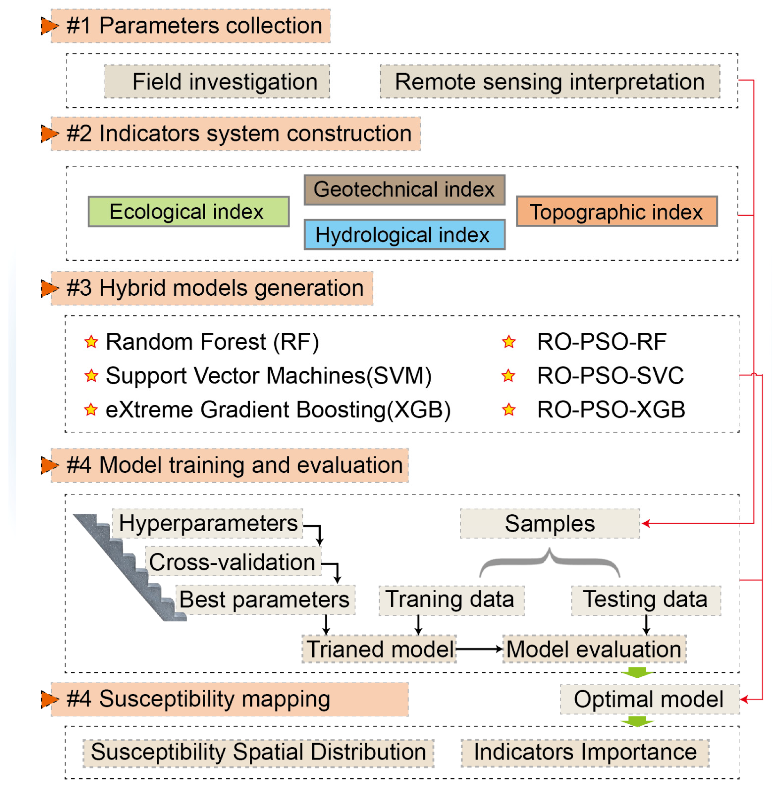
This paper proposes new hybrid methods for assessing debris flow susceptibility coupled with ecohydrological activation from the perspective of debris flow formation, which includes several parts: parameter collection, indicator system construction, hybrid model generation, evolution calculation of model hyperparameters, model training, optimal model determining, and susceptibility assessment.
Figure 2 depicts the flow chart that represents this process.
3.1. Catchment Boundaries Division
The catchment unit is a self-contained hydrological area, with the river serving as the mainline and the water division acting as the boundary [
42]. Catchment units having more physical, geological, or geomorphological significance than grid cells are better suitable for predicting debris flow occurrence [
21,
43]. Furthermore, in terms of debris flow formation, activities such as material source initiation, debris flow movement, erosion, and deposition all occur within catchment units. As a consequence, catchments were selected as mapping units for this research. As illustrated in
Figure 3, the Dadu river basin is divided into a total of 1780 catchments using GIS spatial analysis tools with the DEM (30 m resolution).
3.2. Inventory of Debris Flows
In recent years, several field investigations on debris flow disasters in the Dadu River basin have been conducted. However, due to its complex topographical conditions and massive area, it is hard to perform an investigation that spans the whole Dadu River basin. Given that remote sensing interpretations allow for flexibility and low labor costs [
44], this study utilized high-resolution remote sensing images to perform visual interpretations, giving an abundance of data for model training. Distinguishing factors such as vegetation changes, landslide scar(s), and clear channel visibility were fully considered in this interpretation procedure to ensure the reliability of the interpretation outcomes [
45]. Finally, 562 catchments were picked from the 1780 catchments to train the hybrid machine learning models, with a total of 281 catchments identified in the study area as being prone to debris flow (DFs), and the remaining 281 catchments as being not prone to debris flow (NDFs).
3.3. Establishment of an Indicator System Coupled with Ecohydrological Activation
The selection of predictor factors is crucial in predicting the susceptibility of debris flows [
36,
46]. The debris flow formation process can be split into several stages based on the physical formation mechanism, such as accumulation of loose materials, initiation driven by rainfall, dynamic movement controlled by terrain and channel conditions, and accumulation at the outlet [
47,
48,
49]. Based on the aforementioned factors, this article presents a debris flow susceptibility indicator system coupled with ecohydrological activation from the standpoint of physical mechanisms, taking into account the comprehensive effects of vegetation, such as the positive effect of root anchoring and the negative effect of vegetation weight loads, on the slope failure from the physical mechanism. Overall, the structure of this new indicator system (
Figure 4) is designed based on the debris flow formation mechanism and general disaster-causing factors used in traditional debris flow susceptibility methods, and the indicator system consists of ecological indexes, hydrological indexes, geotechnical indexes, and topographic indexes. The processed data of this research and their sources are presented in
Table 1. To ensure the consistency of spatial resolution among all data, the feasibility of parameter calculation, and the applicability of the accurate topography depicted in the DEM to the debris flow susceptibility assessment [
50], all data from different sources were resampled to the same spatial resolution as the DEM (30 m) using the GIS platform’s resampling tool. Due to the need for machine learning input parameter formats, the GIS platform’s Zonal Statistics tools were then used to obtain the feature statistics (such as the mean or majority) of each catchment.
3.3.1. Ecological and Hydrological Indexes
(1) Vegetation weight loads (VWL) and root morphology (RM).
Vegetation is the producer in the food chain in terrestrial ecosystems; it transports materials and energy through the ecosystem and is directly tied to the creation of the natural environment [
53]. The vegetation in the studied region has obvious vertical and horizontal zonality, which is assisted by the topographically extreme belt conditions; distinct vegetation species with differing vegetation weight loads and root morphologies are concentrated at different altitudes [
54,
55]. Given that root reinforcement and vegetation weight loads are important in the stability evaluation of vegetation-covered slopes [
54,
56], and that shallow landslides are one of the main material sources of debris flows, vegetation weight loads and root morphology are included as ecological indexes in the debris flow susceptibility assessment indicator system. The root morphological properties of various plant types in the research region were collected via field investigations (
Table 2), and the quantitative techniques and details of the vegetation weight load calculations were found to be similar to those employed by Zou et al. (2021b) [
8].
(2) Flow depth (FD) and runoff velocity (RV).
Water is not only the main triggering factor of debris flow formation, but it is also a fundamental component of the debris flow; hence, hydrological conditions are important for debris flow formation. The flow depth and runoff velocity at a gully’s mouth are the overall outcomes of a dynamic hydrologic process that involves rainfall, water storage, depression filling, overflowing within the slope area, and channel confluence [
57,
58]. To some degree, these characteristics reflect the catchment’s topographic relief, the complexity of the gully morphology, and the roughness of the gully base. As a result, to represent the hydrodynamic properties of the runoff in the assessed river branches and channels, the flow velocity and runoff depth are included as hydrological indicators in the susceptibility indicator system. However, the study area is too large to use electronic equipment to monitor flow velocity and runoff depth in each catchment. To compensate for this deficiency, index values based on five assumptions were derived to substitute real flow velocity and depth measurements:
A constant rainfall intensity,
The water input from rainfall is equal to the output in the catchment,
The effect of potential energy is considered, and the work done by resistance is ignored,
The influence of different water depths on potential energy is ignored, and
Water particles at the same elevation arrive at the gully mouth at the same time.
According to assumption 1, the rainfall per unit time is equal to the volume of water output from the basin and can be deduced as follows:
where
P is the rainfall intensity;
A is the watershed area;
Q is the discharge at the outlet; and d
t is the unit of time.
Since resistance and the effect of the water depth on the potential energy are ignored, all gravitational potential energy is converted into kinetic energy. Therefore, the following formula is given for any particle:
where
m is the mass of the water particle;
g is the acceleration of gravity;
h is the height difference between the water particle and the point at the gully mouth; and
v is the particle velocity at the gully mouth.
The initial potential energy of particles that flow to the gully mouth at the same time is calculated as follows:
where
ρ is the density of water;
L(h) is the length contour line where the relative height is
h; and
B(h) is the horizontal displacement of the contour line.
The average kinetic energy of particles that flow to the gully mouth at the same time is calculated using Formula (5):
The runoff velocity is calculated as follows:
The flow depth is calculated as follows:
where
b is the average width of the wet crossing section and
S is the area of the wet crossing section.
3.3.2. Geotechnical and Topographic Indexes
(1) Thickness (ST) and strength (SS) of the soil mass.
The direct reason for the formation of unstable slopes is that the impervious-layer soil shear strength is less than the sliding force of the soil mass, which contributes to the formation of landslide disasters [
59,
60]. Therefore, the soil shear strength and soil mass thickness, related to the depth of the impervious layer, are included as geotechnical indicators in the susceptibility prediction index system. Here, the soil shear strength refers to the ultimate strength of the soil mass against shear failure. According to the Mohr–Coulomb failure criterion [
61], this variable is calculated using the following formulas:
where
and
are the shear strength (kPa) and cohesion (kPa) of the soil mass, respectively;
and
are the friction angle (°) and density (t/m
3) of the soil mass, respectively;
is the normal stress of the soil mass (kPa); and
z is the elevation difference from the surface of the soil mass to the bedrock surface (m).
(2) Altitude difference (AD) and channel gradient (CG).
Topographical factors have a considerable impact on the initiation and dynamic process of debris flow formation [
62,
63]. The steep channel and enormous relief may give an abundance of potential energy conditions for debris flow formation [
20]. As a consequence, general topographical characteristics such as altitude difference and channel gradient are included in this index system for assessing debris flow susceptibility. The altitude difference (AD) between the catchment’s top and outflow shows the catchment’s overall potential energy conditions [
64]. The channel gradient (CG) reflects the channel’s overall steepness and is computed by dividing AD by the channel length [
65].
(3) Connectivity index (IC) and propagation probability index (PPI).
The formation of a debris flow requires not only an abundant water source and loose material conditions but also steep topographic conditions that are conducive to the movement of the debris flow [
66]. The lower the stability of a slope with loose material in the source area, the higher the terrain connectivity from the source area to the gully mouth, and the more conducive the conditions to the formation of a debris flow. Therefore, the propagation probability index and connectivity index are incorporated as topographic indexes into the debris flow prediction index system.
The propagation probability index calculated by the Flow-R model [
67] provides the probability of the unstable materials propagating to a point likely to be reached by debris flows. The Flow-R model’s key input parameters are a digital elevation model (DEM) and the loose material source area. The procedure identifying the source area considers the mechanical anchoring effect of the root system and the vegetation weight loads on the slope covered with various vegetation types. Details and results of the propagation probability index computation can be acquired by referring to Zou et al. (2021b) [
8].
The connectivity index was used in this study to represent the potential connectivity between the outlet and other parts of the catchment, and can be quantified by the spatial analysis tools in geographic information systems (GIS). According to Equation (13), its input parameters include land-use data (at a 30 m resolution) and a DEM (at a 30 m resolution) [
68,
69].
where
ICk is the connectivity index;
Dup is the potential of sediments moving from the upstream channel to the downstream channel;
Ddn is the possibility of sediments reaching the outlet through the flow path;
is the average weight of the upslope catchment area determined by the land-use type;
is the average gradient of the upslope catchment area;
is the square root of the upslope catchment area;
𝑑𝑖 is the length of the flow path from the debris source area to the
ith unit; and
and
are the weight and the gradient of the
ith unit in the watershed, respectively.
3.4. Parameter Preprocessing
3.4.1. Analysis of Selected Characteristics’ Collinearity
Characteristics’ collinearity in machine learning modeling indicates that two or more features contain similar information, i.e., there is a strong correlation between them, and that strong collinearity may cause model instability [
20,
35,
38]. The Spearman correlation analysis technique was used to compute the correlation coefficients (
Figure 5) in this research. There were two pairs of variables with strong relationships, with correlation coefficients of 0.83 for RM vs. VWL and 0.82 for ST vs. SS. As a result, RM and ST were eliminated.
3.4.2. Data Standardization
The indexes involved in the index system can be quantified according to the calculation methods described above based on the field investigations and collected documentation. Furthermore, considering the direct use of data with different orders of magnitude and dimensions for training affects the accuracy of the model [
70], these indexes were standardized using Formula (14) to accelerate model convergence and improve the model accuracy [
20].
where
Ifinal is the index value after standardization;
I is the index value before standardization;
Imin is the minimum index value; and
Imax is the maximum index value.
Finally, some quantified indexes involved in the index system are shown in
Figure 6a–f.
3.4.3. Generating the Cross-Validation Dataset
There is still a chance of overfitting on the test set because the parameters may be changed until the estimator performs optimally when testing multiple settings (“hyperparameters”) for estimators, and the cross-validation algorithm in Scikit-learn was thus used to build the cross-validation dataset. As a consequence, the model may be trained with different subsets of training data before being tested with the test dataset, avoiding overfitting. In this work, 70% of the sample set was used to construct the cross-validation dataset (
Figure 7), with the remaining 30% used for final model validation.
3.4.4. Removing Outliers (RO)
Outliers are abnormal values in a dataset, and the goal of integrating the RO algorithm with the machine learning model in this study was to eliminate outliers from the input dataset since their existence is often caused by human errors caused by the data collection, recording, or input procedure, or to natural error. The removing outliers procedure improves the capacity to fit and mine the main relationships between debris flow occurrence and disaster-causing factors by reducing noisy data learning in the machine learning model [
71,
72]. As a consequence, the operation of removing outliers from the original data was performed in this study before training the hybrid machine learning models. According to the Pauta criteria [
73], the process of removing outliers is separated into two steps:
Step 1: When the data obey a normal distribution, values outside 3δ from the mean are discarded since this is a small probability event.
Step 2: For the remaining data that do not obey a normal distribution, data outside x δ from the mean are determined to be outliers. The δ is the standard deviation, and the value of x needs to be decided depending on expert experience and the actual situation.
3.5. Machine Learning Algorithms
Due to the abundance of datasets available from remote sensing interpretations, the use of machine learning methods to interpret patterns or extract information from data [
74] is increasing for mountain disaster prediction. These machine learning algorithms, such as support vector machines (SVMs), eXtreme Gradient Boosting (XGB), and random forest (RF) [
33,
35,
36], were selected as the basis of hybrid machine learning methods and then combined in a hybrid with the RO algorithm and hyperparameter optimization algorithm.
3.5.1. Support Vector Machines (SVMs)
SVM is a general term for some classifiers that are used to solve the separation hyperplane with the maximum interval on the feature space, with interval maximization as the learning strategy [
20,
34]. The hyperplane is a linear subspace with the residual dimension equal to 1 in the n-dimensional Euclidean space and is used to split the feature space into two half-spaces [
75]. In this study, support vector classification (SVC) was selected.
3.5.2. Random Forests (RF)
Random forest (RF) is one of the ensemble-learning approaches commonly used for assessing debris flow susceptibility [
36]. This technique improves the decision tree algorithm by integrating numerous decision trees, the formation of which is based on samples chosen independently [
33]. To be more specific, some samples are drawn at random from the original training sample set, and then a series of decision trees are created to build the random forest based on the decision rules. Finally, the classification results of the new data are computed based on the number of votes cast by the decision trees. As a result of the random selection of features and samples during each decision tree training, random forest (RF) is distinguished by strong noise resistance and steady performance.
3.5.3. eXtreme Gradient Boosting (XGB)
XGB is a cutting-edge machine learning approach for debris flow susceptibility that quickly implements the Gradient Boosting Decision Tree (GBDT) algorithm and adds many refinements to it, integrating several tree models to construct a strong classifier [
20]. The technique is several times quicker than conventional algorithms due to the massively parallel boosting tree, and it has superior computational accuracy since XGB conducts a second-order Taylor expansion on the loss function, whereas common algorithms only use a first-order Taylor expansion. XGB was thus chosen for this investigation.
3.6. Particle Swarm Optimization (PSO)
The particle swarm optimization (PSO) algorithm is a biological heuristic method in the realm of computer intelligence that is often used for intelligence optimization [
38]. The PSO algorithm is inspired by the study of bird feeding behavior, and reflects an effective and easy method used by birds to hunt for food by looking in the area nearest the food. The particle is likened to a bird in that it decides its next move based on its own experience and the best experience of its companions. The progression of its movement is summarized in Equations (16) and (17).
where
m is the number of current iterations,
and
are the position and velocity of
ith particle in the
mth iteration in the feature space,
and
are random number of values between 0 and 1,
and
are learning factors,
is the inertial weight coefficient,
is the personal best position of particle
i in the
mth iteration, and
is the best position of all particles.
3.7. Generating the Hybrid Machine Learning Models
In this study, the procedure of integrating each machine learning model with RO and PSO consists of two steps:
Step 1: The RO algorithm removes outliers from the input dataset because their presence is often attributable to human mistakes or to natural error. The goal of this step is to improve the capacity to fit and mine the main relationships between debris flow occurrence and disaster-causing factors by reducing noisy data learning in the machine learning model. As a result, the operation of removing outliers is important.
Step 2: The dataset that has been processed by the RO algorithm is then utilized to train the machine learning model. Some parameters, known as hyperparameters, must be artificially set in the traditional training process of machine learning models. The traditional hyperparameter debugging procedure cannot easily locate the optimal hyperparameters from all parameter groups due to time and labor costs, particularly when the hyperparameters can be parameters of the floating-point type. To address this shortcoming, the PSO algorithm is used to optimize the selection of hyperparameters. By integrating with the PSO algorithm, the computer can automatically calculate the optimal hyperparameters of machine learning algorithms, avoiding the intervention of human subjective factors.
Finally, hybrid machine learning models, including RO-PSO-SVC, RO-PSO-RF, and RO-PSO-XGB, were established by integrating the aforementioned machine learning algorithms with the remove outliers (RO) operation and the PSO algorithm, which boosts the model’s fitting accuracy and stability. The efficacy of the RO operation in hybrid model construction was evaluated further by comparing it to several hybrid models that just use PSO, such as PSO-SVC, PSO-RF, and PSO-XGB.
3.8. Model Training and Evaluation
The relationship between disaster-causing factors and debris flow occurrence can be quantified by model training with a set of weights and bias parameters of machine learning models. However, the hyperparameters of conventional machine learning models have to be artificially tuned, and the debugging process is subjective and highly dependent on the experience of experts. In this article, the particle swarm algorithm (PSO) is used to look objectively for the optimal super parameters for PSO-RF, PSO-SVC, PSO-XGB, RO-PSO-RF, RO-PSO-SVC, and RO-PSO-XGB, with mean squared error (
MSE) and root mean squared error (
RMSE) closest to 0 and prediction accuracy (
ACC) (Formula (18)) scores closest to 1. Additionally, the spatial consistency of these debris flow susceptibility results produced by different models needs to be evaluated using Spearman’s rank correlation coefficients, since a similar susceptibility result obtained by different approaches indicates that these results are reliable [
36,
76]. To assess the effectiveness of these six hybrid models, the
ACC,
MSE,
RMSE, and the time consumed for hyperparameters optimization were recorded (
Table 3). According to
Table 3, RO-PSO-SVC has the greatest performance with a test data ACC of 0.946. The area under the curve (AUC) was also calculated to estimate the performance of the models using the receiver operating characteristic (ROC) curve [
77,
78], as shown in
Figure 8. The higher the AUC value, the better the prediction performance of the model. The prediction accuracy (
ACC) (Formula (3)) is a rate of correct assignment for test samples.
where
TP and
TN show the number of properly identified catchments, whereas
FP and
FN show the number of wrongly categorized catchments (
Table 4).
The
MSE and
RMSE are used for estimating the generalization error of the model, and can be expressed as follows:
where
represents the observed values in the training dataset or validation dataset,
represents the predicted values from the debris flow susceptibility models, and
n is the total number of the samples in the training or validation datasets.
4. Results
Using the techniques described above for parameter optimization, optimal models with matching hyperparameters (
Table 3) were identified and used to predict the susceptibility of debris flows. The spatial consistency of the debris flow susceptibility maps for the different optimal models noted above was thus analyzed using Spearman’s rank correlation coefficients. The Pearson correlation coefficients range from 0.86 to 0.98 (
Figure 9), indicating that the index system presented in this article can predict the occurrence of debris flows in the topographically extreme belt, and the results are reliable and effective. The outputs of the aforementioned hybrid or non-hybrid models were used to reclassify susceptibility levels into five groups (very low, low, medium, high, and very high) using the natural break classification technique [
36]. Susceptibility maps were then generated on the GIS platform for visualization (
Figure 10). The findings reveal that those catchments with high and very high debris flow susceptibility are most prevalent in the study area’s central mountainous region, whereas the northern plateau areas with gentle topographical change have lower susceptibility. Compared with the distribution of the susceptibility maps (
Figure 10) obtained by different models, the findings show that the catchments with different susceptibility levels tend to be clustered together with greater spatial continuity after integrating the machine learning models used in this article with the RO and PSO algorithms. This may be because the RO and PSO algorithms enhance the machine learning model’s ability to fit and mine the major relationships between debris flow occurrence and disaster-causing factors by reducing noisy data learning and hyperparameter optimization.
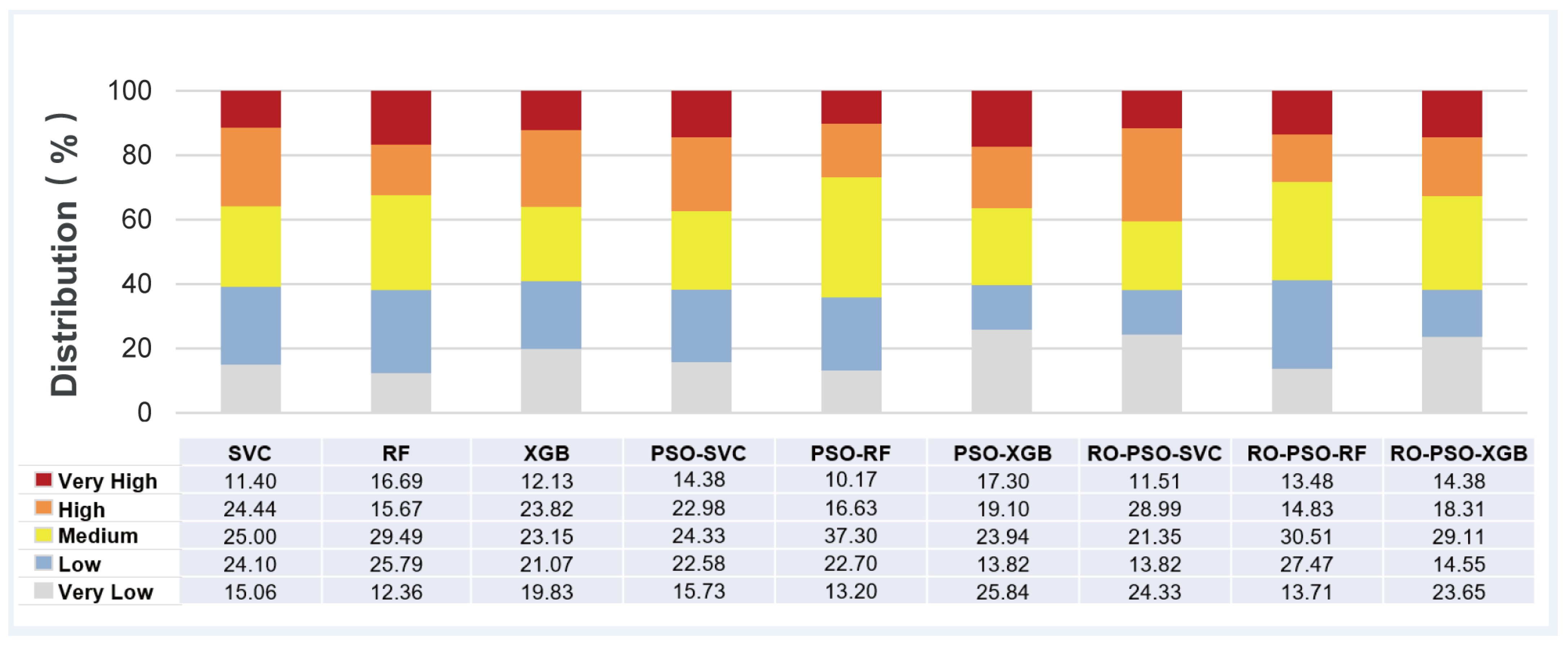
Figure 11 depicts the relative distribution of each model’s different susceptibility levels. The high level has the highest percentage (28.99%) in the RO-PSO-SVC model, with the remaining 24.33%, 13.82%, 21.35%, and 11.51% of watersheds falling into the very low, low, medium, and very high susceptibility levels, respectively. The percentages of the total of low and very low for all of the above-mentioned models’ debris flow susceptibility maps are quite close to 38.85%. Furthermore, the main classes in the research region include medium, high, and extremely high debris flow susceptibilities.
5. Discussion
This study proposes new hybrid machine-learning approaches combined with the removing outliers (RO)algorithm and the particle swarm optimization (PSO) algorithm to predict the susceptibility of debris flows in the Dadu River basin, a typical extreme topography transition belt on the eastern margin of the Qinghai-Tibet Plateau. The PSO and RO algorithms were implemented in these hybrid models to identify the perfect hyperparameters for the machine learning model and to lessen the impact of noise on the model’s convergence speed and prediction accuracy. The model performance evaluation analysis (ACC) revealed that machine learning models enhanced by the PSO and RO algorithms outperformed solo machine learning models. According to the ACC analysis, the RO-PSO optimization algorithms improved the performance of SVC, RF, and XGB by 3.84%, 2.59%, and 5.94%, respectively. The ACC value of SVC, RF, and XGB rose by 2.63%, 0.56%, and 1.34%, respectively, when only the PSO algorithm was used. Furthermore, the RO algorithm improved the performance of PSO-SVC, PSO-RF, and PSO-XGB by 1.21%, 2.03%, and 4.60%, respectively. The improvement in the performance of these machine learning models shows that the indicators can shed light on the physical mechanisms behind the debris flow formation, such as the physical failure mechanism on vegetation-covered slopes revealed by the index PPI. Another point worth noting is that the degree of RF improvement is not obvious after integrating only with the PSO algorithm. Results analysis showed that the PSO algorithm can significantly improve the performance of machine learning models with floating-point-type super parameters, such as SVC and XGB, since the PSO algorithm has a stronger parameter search capability for floating-point-type super parameters than for integer super parameters. The greater the number of floating-point-type super parameters in the model, the greater the performance benefit. As a result, the fact that the major super parameters for RF debugging in this study were all integer types restricts the PSO algorithm’s ability to improve.
RO-PSO-SVC has the strongest spatial recognition capacity to identify debris flow hazards among all of the aforementioned models, as its total percentage of debris flow catchments (
Figure 12) with high and very high susceptibility is the biggest, accounting for 91.04%. Interestingly, we found that RO-PSO-SVC and RO-PSO-XGB result in fewer false alarms than RO-PSO-RF, with a lower total percentage (1.44%) of debris flow catchments with very low and low susceptibility levels. RO-PSO-XGB, by comparison, classifies more debris flow as medium susceptibility than RO-PSO-SVC. In this regard, RO-PSO-SVC is better able to minimize false alarms since the total percentage of debris flow catchments with very low, low, and medium susceptibility is 8.96%, compared to 11.47% for RO-PSO-XGB.
RO-PSO-SVC also has the best performance for predicting debris flow susceptibility, according to the model performance evaluation analysis (
ACC,
MSE, and
RMSE), and was thus chosen to interpret and diagnose the contribution of different predictor factors. SHAP (SHapley Additive exPlanations) [
79], a game-theoretic technique to explain the output of any machine learning model, can quantify the relative importance of each causal factor.
Figure 13 shows that runoff velocity (RV) is the most significant predictor variable in the RO-PSO-SVC model, with a relative importance value of 49.57%, and flow depth (FD), the associated predictor variable representing hydrological conditions, has a relative importance value of 8.45%. Topography-related factors such as AD, CG, IC, and PPI have a relative relevance of 11.08%, 9.05%, 4.26%, and 3.33%, respectively. Such results suggest that topography and hydrology play important roles in debris flow formation as general factors, which is consistent with previous research [
34,
35,
36] in topographically extreme belts. Furthermore, the factor importance analysis shows that the ecology-related factor, vegetation weight loads (VWL), has a relatively low contribution to the debris flow occurrence, which is similar to the findings of previous studies [
35,
36] that revealed that ecology-related factors reflecting vegetation cover, such as Normalized Difference Vegetation Index (NDVI), contribute less to debris flow formation than topography- and hydrology-related factors, taking the Sichuan province as the study area.
The top three indicators with the greatest contribution according to
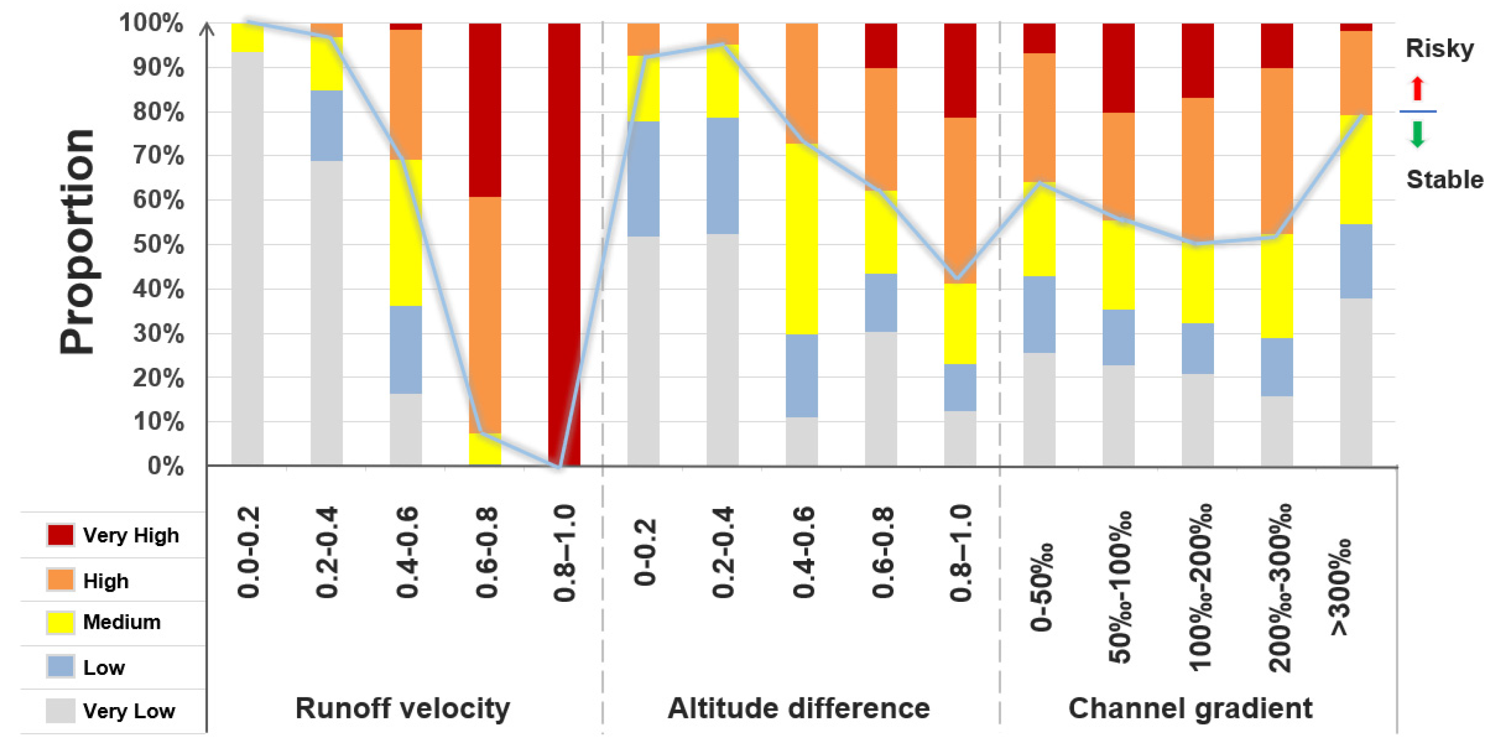
Figure 13 were selected for further statistical analysis to investigate the impact of triggering factors on debris flow occurrence.
Figure 14 depicts the proportion of catchments with different debris flow susceptibility (as predicted by RO-PSO-SVC) for each level of different triggering factors. This shows that there is an obvious positive correlation between the factors of runoff velocity and altitude difference with debris flow occurrence, because the catchments with high and very high susceptibility levels are concentrated in the catchments with a greater runoff velocity index and a greater altitude difference index. The performance of altitude difference is easy to understand since the enormous relief may provide an abundance of potential energy conditions for the formation of debris flows. After deep analysis, we attribute the strong sensitivity of the runoff velocity factor to the debris flow occurrence to the good ability of this index to represent the process of debris flow formation, which indicates that there is strong link between the physical movement mechanism used in the derivation process of the runoff velocity index and the dynamic process of debris flow movement. The factor of channel gradient also plays an essential role, as implied in
Figure 14. The total proportion of catchments with very high and high susceptibility in 100–200‰ of the channel gradient is 49.60%, the highest of all channel gradient levels. This result is consistent with the findings of Xiong et al. (2020) [
36], who conducted debris flow susceptibility research in the Sichuan Province.
It is worth noting that the susceptibility classification results show that there is a high proportion of catchments with high and very high susceptibility in the study area, which is consistent with the study results of Xiong et al. (2020), who explain that this is because this region belongs to the transition belt, where the topography varies enormously, from the Qinghai–Tibet Plateau to the Sichuan Basin, and is coupled with dry valleys and fault zones. Another point of concern is that, although the study improved the performance of the debris flow susceptibility assessment by introducing some factors related to physical–mechanical mechanisms, the computation of these factors was time consuming, particularly for the PPI reflecting the physical failure mechanism on vegetation-covered slopes, which took nearly a month to compute with 26 computers. As a result, the next stage of the research will look for methods to lower the computing costs associated with introducing parameters related to physical–mechanical mechanisms at the regional scale.
It is well known that the physics behind the debris flow formation are closely related to the accumulation of loose materials, initiation driven by rainfall, the potential of dynamic movement controlled by terrain and channel conditions, and accumulation at the outlet. From the viewpoint of indicator selection, all indicators used in this research are focused on the physical mechanisms behind debris flow formation, such as the failure mechanisms of the vegetated slope and the dynamic processes of debris flows. As a result, the main contribution of this paper is to propose a regional-scale susceptibility index system for predicting the probability of debris flow occurrence in the Dadu River basin, a typical extreme topography transition belt on the eastern margin of the Qinghai-Tibet Plateau, from the perspective of the debris flow formation mechanism. This system takes into account not only the common geographic features (such as enormous topographic relief and active tectonics) that control the occurrence of debris flows, but also the comprehensive impacts of vegetation on the occurrence of debris flows, such as the positive effect of root anchoring and the negative effect of vegetation weight loads. In this respect, this study is innovative and essential for the development of regional-scale debris flow susceptibility evaluation. To ensure that the causal factors selected in this study stand up to scrutiny, these indicators were classified into different categories, as is commonly done in the traditional methodology. This was undertaken to ensure that the primary concept of constructing the indicator system in this article was based on three fundamental disaster-causing factors that control debris flow formation, namely, topographic condition, hydrological condition, and material condition. Furthermore, the novel hybrid models formed by integrating the machine learning model with RO and PSO algorithms were, for the first time, also used in the catchment-based assessment of regional-scale debris flow susceptibility. These hybrid models with good performance also provide a scientific reference for future regional-scale debris flow susceptibility assessments.


 ,
, 


