Method for Estimating the Optimal Coefficient of L1C/B1C Signal Correlator Joint Receiving

Abstract

The design of a modern Global Navigation Satellite System (GNSS) has been exceptionally valued by the military and civilians of various countries. The inclusion of the pilot channel in addition to the navigation data channel is considered one of the major changes in GNSS modernization. Schemes of an equal weight combination (1:1 combination) and power ratio combination for data and pilot are primarily adopted by traditional receivers. With the emergence of the new data and pilot modulation signals with unequal power, such as L1C at Global Positioning System (GPS) L1 frequency and B1C at BeiDou Navigation Satellite System (BDS) B1 frequency, the traditional combination coefficient cannot achieve optimal reception performance. Considering the influence of the combination coefficient on the reception performance, the optimal coefficient of the correlator joint is estimated in this paper. The entire architecture of the data/pilot correlator joint tracking and positioning with unequal power is given. Based on the equivalence principle of the correlator joint and the discriminator joint, the optimal coefficient of the carrier loop is determined. A mathematical model of joint code tracking accuracy is established, and the optimal coefficient of the code loop is determined. The real-life satellite signal and simulation results show that the amplitude–ratio combined scheme is the best for receiving of correlator joints, followed by the power–ratio combination scheme and, finally, the 1:1 combination scheme. It is worth mentioning that the positioning accuracy of the amplitude–ratio combination is improved by 2% compared to the 1:1 combination, and by 1.3% compared to the power–ratio combination for B1C signal. The positioning accuracy of the amplitude–ratio combination is improved by 2.37% compared to the 1:1 combination, and by 1.6% compared to the power–ratio combination for L1C signal. The conclusions of this paper are validated for the traditional data/pilot with an equal power allocation. The techniques and test results provide technical support for GNSS high-precision-user receivers.

1. Introduction

The growing demand for location, navigation and positioning services is boosting the development of high-utilization ratio signals, which have been developed by a new generation of global navigation satellite system (GNSS). Compared with traditional navigation signals, pilot channels appear in modernized navigation signals, such as GPS-L2C, GPS-L5C, Galileo satellite navigation system (Galileo)-E1, Galileo-E5, Galileo-E6OS, BDS3 -B2, Global Navigation Satelite System (GLONASS)-G3OC signal [1,2,3]. The navigation message is loaded on the data channel, and the pilot channel is only loaded with the spreading code. Such a signal structure not only improves the receiving performance, but also promotes improvements in the receiving method.

Following this trend, many works have emerged on research and development toward the reception of GNSS signals with pilots; the typical algorithms currently include pilot-assisted data and the joint reception of pilots and data. To maximize the positioning accuracy of navigation signals, high-precision user receivers consider the advantages of data and pilot components for positioning. The pilot component with a better tracking performance and higher power is used for ranging, and then the loop tracking result is used to assist the data component in calculating the navigation message information. This algorithm has low complexity but fails to make full use of the design performance of the Multiplexed Binary Offset Carrier (MBOC) signal [4,5]. Therefore, some scholars combine data and pilot components to achieve the best positioning performance. For example, there are non-coherent combination algorithms, differential combination algorithms and coherent combination algorithms for the joint acquisition of data/pilot [6,7,8,9,10]. There are also many scholars who have studied the joint tracking method of data/pilot. In 2005, Oliver proposed the joint tracking method of the future data/pilot signal carrier loop of GNSS, adopted a combination of discriminators, and provided the calculation method for the coefficients [11]. References [12,13] studied the performance of carrier frequency combination tracking for GPS L2C. Existing methods that discriminators combine for the data and pilot are analyzed in detail. Reference [14] analyzes and proposes a new method based on the joint tracking of data and pilot instead of discriminators; the proposed method removes the navigation data of the data channel through a newly designed navigation data prediction module, and then the correlator integration results of the data and the pilot are coherently combined using an equal weight ratio. The coherent integration result contains the energy of both the data and pilot. Compared with previous methods, this method has no power consumption and does not require additional computational resources. Ref. [15] proposed a tracking method using a data and pilot combination of the GPS L5 signal after a code tracking loop discriminator and filter. Xu D from Tsinghua University discussed the tracking threshold and tracking accuracy of the GPS-L5 signal in correlator joint tracking, discriminator joint tracking, and filter joint tracking. The results show that the correlator joint tracking has the highest tracking accuracy for the carrier loop; the filter joint has a slightly better tracking accuracy for the code loop only when the signal-to-noise ratio is low. However, the correlator joint has the lowest complexity, since only one set of discriminators and filters are needed in the loop. Refs. [16,17,18] achieved a linear union at the output of the discriminator for the acquisition and tracking of GalileoE1 signals. Reference [17] coherently combines the integration results of the E1B and the E1C in a 1:1 ratio, which simplifies the receiver, and the simulation validates its outstanding performance. The above references are all studies on the data/pilot with equal power allocation.

To ensure that global users obtain the best service performance while minimizing terminal costs, a new implementation of MBOC-modulated signals was proposed on civil interoperability signals, realizing that BDS B1C signals are interoperable user levels with GPS L1C and Galileo E1OS [19,20,21,22]. In particular, the three implementations corresponding to pilot and data components have been proposed to comply with the composited BOC (CBOC) modulated on Galileo E1, the time multiplexed BOC (TMBOC) modulated on GPS III L1, and the orthogonal multiplexed BOC (QMBOC) modulated on BDS III B1 [23,24]. These three designs of MBOCs have different transmission and reception performances to ensure compatibility. Among the three MBOC signals, GPS-L1C and BDS-B1C adopt the signal modulation method, in which the power of the data and pilot channels is not equal, at 1:3. The conclusions, based on an analysis of the data/pilot joint receiving algorithm with equal power, cannot be completely applied to situations where the powers of the two are not equal by simple derivation, which attracts researchers to study joint reception of the data/pilot with an unequal power distribution in more depth. The weighting coefficient of the traditional discriminators joint algorithm is determined by the variance in the loop noise, which depends on the power ratio of the data/pilot. Therefore, the traditional discriminator joint algorithm adapts to the data/pilot with an unequal power distribution. For example, Refs. [25,26,27] introduced the combined method of BDS3 B1C signal discriminator output with the power weighting coefficient determined by the variance in the loop noise. The traditional correlator combination is superimposed with the integration results of the data and the pilot, which cannot show the optimal performance in cases where the two powers are not equal. However, there are still some works that use the traditional methods. For example, Refs. [28,29] introduced the traditional correlator coherent and non-coherent joint acquisition and tracking method with consistent power distribution methods for GPS L1C signals, which directly superimpose the results of the correlator integration by equal weight ratio after the symbol decision. It was concluded that a better acquisition performance and tracking sensitivity were still obtained than single-component receivers. Later scholars made some changes to the coefficients of the correlator joint. Acquisition and tracking of correlator joint based on the data/pilot power ratio are introduced in [30,31,32], and the receiving performance is improved. Reference [30] is a coherent joint tracking algorithm based on the L1C and L1CA correlators, and proposes a weighted joint determined based on the signal power ratio to minimize noise. To maximize the advantages of the correlator joint, Reference [33] proposed an improved non-coherent power-weighted joint acquisition algorithm. The least squares method is used to fit the optimal weighting coefficient based on the false alarm rate and monitoring probability of the joint acquisition. It is concluded that the optimal weighting coefficient is related to the received signal strength and power distribution ratio. However, the carrier-to-noise ratio (C/N0) cannot be obtained until the receiver has completed acquisition and tracking. Therefore, an optimal acquisition performance cannot be obtained for the real-time received signal. Ref. [34] analyzed the acquisition performance difference between the power ratio weighting coefficient and the optimal weighting coefficient to be less than 0.5 dB based on Ref. [33]. To avoid the complexity of the receiver, it is recommended that the user select the power ratio weighting coefficient. These references are based on the optimization combination coefficients discussion of acquisition. The correlator joint tracking for unequal distributions of data and pilot power remains in the stage with an equal weight combination (1:1 combination) and power ratio combination, which does not cover the introduction and verification of the positioning module.

To meet the trends of high-precision users, this paper proposes an entire correlator joint tracking and positioning structure, primarily based on the data and pilot signal models with an unequal power allocation. The optimal coefficients of the correlator joint for carrier loop are deduced based on the equivalence of the correlator joint and the discriminator joint. Next, a joint code tracking accuracy model is established for MBOC and BOC signal, and the optimal coefficients of the code loop are determined with the aid of numerical simulation. Finally, the optimal coefficients estimated in this paper are verified by the errors in the carrier loop discriminator, the code loop discriminator, the signal carrier-to-noise ratio and the positioning error. The positioning accuracy improvement ratio of the satellites that participate in the positioning of the BDS3 constellation and the Japanese Zenith satellite (QZSS) constellation was quantified using the correlator joint optimal coefficient and compared with the traditional coefficient.

2. The Mathematical Model and Characteristics of the B1C/L1C Signal

China, the United States and the European Union proposed a new implementation of MBOC-modulated signals on civil interoperability signals, realizing that BDS B1C signals are interoperable at the user level with GPS L1C and Galileo E1OS. These three satellite navigation systems now have broadcast MBOC (6,1,1/11) signals. The MBOC signal modulated on the GNSS system, denoted as MBOC (6,1,1/11), is specified by its power spectral density (PSD), which is a mixture of the PSDs of $BO{C}_{\sin }(1,1)$ and $BO{C}_{\sin }(6,1)$ with an appropriate weighting factor $1/11$. $G_{BO{C}_s(m,n)}(f)$ is the normalized PSD of a sine-phased BOC spreading modulation, which is defined by Equation (1) as follows [35]:

$$G_{BO{C}_{\sin }(f_{\mathrm{s}},f_c)}(f)=\frac{{\sin }^2\left(\pi f{T}_C\right){\sin }^2\left(\pi f{T}_S\right)}{T_C{[\pi f\cos (\pi f{T}_S)]}^2}$$

(1)

where $T_C$ stands for the code period and $T_S$ stands for the subcarrier period. Considering the definition of the MBOC (6,1,1/11) signal, the normalized Power Spectral Density (PSD) (pilot and data channel) can be derived by Equation (2) as follows:

$$G_{MBOC}(f)=\frac{10\cdot {\sin }^2\left(\pi f{T}_C\right){\sin }^2\left(\pi f\raisebox{1ex}{$T_C$}\!\left/ \!\raisebox{-1ex}{$2$}\right.\right)}{11\cdot T_C{[\pi f\cos (\pi f\raisebox{1ex}{$T_C$}\!\left/ \!\raisebox{-1ex}{$2$}\right.)]}^2}+\frac{{\sin }^2\left(\pi f{T}_C\right){\sin }^2\left(\pi f\raisebox{1ex}{$T_C$}\!\left/ \!\raisebox{-1ex}{$12$}\right.\right)}{11\cdot T_C{[\pi f\cos (\pi f\raisebox{1ex}{$T_C$}\!\left/ \!\raisebox{-1ex}{$12$}\right.)]}^2}$$

(2)

The power spectrum of the MBOC (6,1,1/11) modulation signal is obtained by mathematical model simulation. Figure 1 shows that the idea behind MBOC (6,1,1/11) modulation is to increase the power of the higher-frequency (6 MHz) on the BOC (1,1).

The LlC signal is also flying on the QZSS satellite, which has the exact same format as the GPS-L1C signal, except for the QZS1 satellite. Both the data and pilot of Japan’s QZS1 satellite are loaded with BOC (1,1) signals. Since the MBOC (6,1,1/11) definition is only in the frequency domain, the BOC (n, n) component and BOC (m, n) component can be combined in any multiplexing way, as long as the final PSD meets the limitation of express Equation (2). GPS/QZSS and BDS have designed three different schemes.

The implementation schemes of “BOC (1,1) + QMBOC (6,1,4/33)” and “BOC (1,1) + TMBOC (6,1,4/33)” were designed for B1C and L1C. According to the power distribution factor and phase relationship in

Table 1. Design scheme of L1C, B1C.

NUM	Signal Name	Modulation	Power Distribution	Phase Relationship
1	B1C	BOC (1,1)	1:3	orthogonal
		QMBOC (6,1,4/33)
2	L1C	BOC (1,1)	1:3	Same (GPS, QZS 2~4), Orthogonal (QZS1)
		TMBOC (6,1,4/33) (GPS, QZS 2~4) BOC (1,1) (QZS1)

, the time domain expression can be deduced in Equations (3) and (4) as follows:

$$S_{B1C}(t)=\frac{1}{2}D(t)\cdot C_{B1Cd}(t)\cdot su{b}_{B1Cd}(t)\cdot \cos (2\pi f_{B1}t)-\frac{\sqrt{3}}{2}{C}_{\sec }(t)\cdot C_{B1Cp}(t)\cdot su{b}_{B1Cp}(t)\cdot \sin (2\pi f_{B1}t)$$

(3)

$$S_{L1C}(t)=\frac{1}{2}D(t)\cdot C_{L1Cd}(t)\cdot su{b}_{L1Cd}(t)\cdot \cos (2\pi f_{L1}t)+\frac{\sqrt{3}}{2}{C}_{\sec }(t)\cdot C_{L1Cd}(t)\cdot su{b}_{L1Cp}(t)\cdot \cos (2\pi f_{L1}t)$$

(4)

2.1. The Characteristic of Autocorrelation

In the navigation receiver, acquisition and tracking are based on the cross-correlation function of the satellite signal and local reproduction signal. Therefore, the signal autocorrelation function is very important in signal reception and processing. The autocorrelation function of the BOC signal is written in the form of a trigonometric function, which is shown in Equation (5) as follows [35]:

$$R_{BO{C}_s(m,n)}(\tau )={\wedge }_{T_s}(\tau )+{\displaystyle \sum _{k=1}^{M-1}{(-1)}^k}(1-\frac{k}{M}){\wedge }_{T_s}(\left|\tau \right|-k{T}_s)$$

(5)

where $T_s$ stands for Subcarrier period. $M=\frac{2m}{n}$ stands for modulation order of the BOC signal. ${\wedge }_L(\tau )$ stands for the trigonometric function, and its mathematical expression is as follows:

$${\wedge }_L(\tau )\stackrel{\Delta }{=}\{\begin{array}{cc}1-\frac{\left|t\right|}{L},& \left|t\right|\le L\\ 0& other\end{array}$$

(6)

According to the design scheme of B1C and L1C, the autocorrelation functions can be obtained as follows:

$$R_{L1Cd}(\tau )=R_{B1Cd}(\tau )=R_{L1Cp(\mathrm{QZS}1)}(\tau )={\wedge }_{T_C/2}(\tau )-\frac{1}{2}{\wedge }_{T_s}(\left|\tau \right|-T_C/2)$$

(7)

$$R_{L1Cp(\mathrm{GPS},\mathrm{QZS}2~4)}(\tau )=R_{B1Cp}(\tau )=\frac{29}{33}\cdot [{\wedge }_{T_C/2}(\tau )-\frac{1}{2}{\wedge }_{T_s}(\left|\tau \right|-T_C/2)]+\frac{4}{33}\cdot [{\wedge }_{T_C/12}(\tau )+{\displaystyle \sum _{k=1}^{11}{(-1)}^k}(1-\frac{k}{12}){\wedge }_{T_s}(\left|\tau \right|-k{T}_C/12)]$$

(8)

The data/pilot joint autocorrelation function for B1C and L1C is deduced as follows:

$$R_{\mathrm{QZS}1}(\tau )={\wedge }_{T_C/2}(\tau )-\frac{1}{2}{\wedge }_{T_s}(\left|\tau \right|-T_C/2)$$

(9)

$$R_{B1C/L1C(\mathrm{GPS},\mathrm{QZS}2~4)}(\tau )=\frac{10}{11}\cdot [{\wedge }_{T_C/2}(\tau )-\frac{1}{2}{\wedge }_{T_s}(\left|\tau \right|-T_C/2)]+\frac{1}{11}\cdot [{\wedge }_{T_C/12}(\tau )+{\displaystyle \sum _{k=1}^{11}{(-1)}^k}(1-\frac{k}{12}){\wedge }_{T_s}(\left|\tau \right|-k{T}_C/12)]$$

(10)

2.2. Code Tracking Accuracy

The general expression of the standard deviation of the code-tracking error produced by the thermal noise of the noncoherent code loop phase detector can be expressed as follows [35]:

$${\sigma }_{tDLL}=C\times \sqrt{\frac{B_L(1-0.5B_L{T}_p){\displaystyle {\int }_{-B_f/2}^{B_f/2}{G}_L\left(f\right){\sin }^2\left(\pi fd{T}_c\right)df}}{{\left(2\pi \right)}^2\cdot (\mathrm{C}/\mathrm{N}0)\cdot [{\displaystyle {\int }_{-B_f/2}^{B_f/2}f{G}_{L,R}\left(f\right)\sin \left(\pi fd{T}_c\right)df{]}^2}}}\cdot \sqrt{1+\frac{1}{T_p}\frac{{\displaystyle {\int }_{-B_f/2}^{B_f/2}{G}_L\left(f\right){\cos }^2\left(\pi fd{T}_c\right)df}}{(\mathrm{C}/\mathrm{N}0)\cdot [{\displaystyle {\int }_{-B_f/2}^{B_f/2}f{G}_{L,R}\left(f\right)\cos \left(\pi fd{T}_c\right)df{]}^2}}}\cdot$$

(11)

where $C$ is the speed of light, $B_L$ is the noise bandwidth of the code tracking loop, $B_f$ is the filter front-end bandwidth, $T_p$ is the coherent integration time, $G_L(f)$ is the power spectrum density of the local reference signal, $G_{L,R}(f)$ is the cross power spectral density of the local signal and the received signal, and $d$ is the correlator interval, $T_c$ is the code period, and $\mathrm{C}/\mathrm{N}0$ is the signal carrier-to-noise ratio. Figure 2 shows the simulated signal noncoherent code-tracking error, where $B_L$ is 5 Hz, $B_f$ is 40 MHz, $T_p$ is 0.01 s.

The tracking accuracy of the QMBOC and TMBOC signal codes as the pilot components overlaps in different C/N0 and correlator intervals. Their code-tracking error is lower than that of the BOC (1,1) signal as a pilot component.

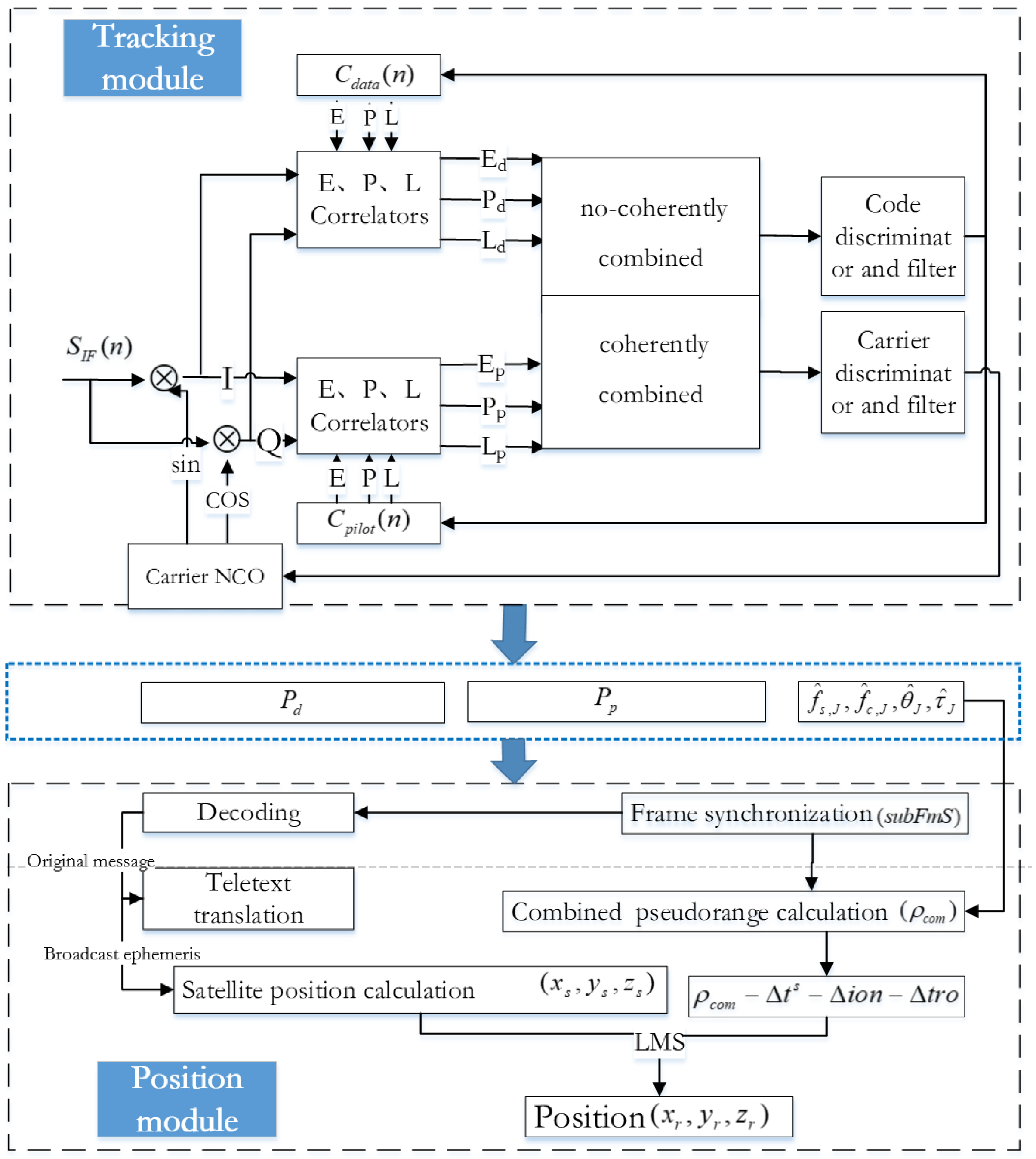
3. The Joint Receiving Scheme of Correlator

3.1. Correlator Joint Receiving Algorithm

A pilot channel undergoes similar path delays and shifts to a data channel, thus making data/pilot combined tracking an attractive option. The two components have the same frequency, and the carrier phase relationship is fixed. The traditional single-component tracking method wastes useful power. Based on the specific relationship between the data and the pilot, the receiver adopts correlator joint receiving, where the total signal power is increased to obtain a higher tracking accuracy. The combination receiving design framework is shown in Figure 3, which includes a tracking module and a positioning module.

In the tracking module, “Costas” is adopted by the data-component carrier tracking loop due to the unknown message information that it modulates. However, a pure phase-locked loop with better performance is designed in the pilot-component carrier loop because it modulates the known secondary code information. After the digital intermediate frequency signal is stripped from the carrier, it is coherently integrated with the early, punctual, and late local copy code.

The receiver correlator outputs early branch E, punctual branch P and late branch L, which can be expressed as follows:

$$E_d=A_{d}D\frac{\sin (\pi {\delta }_{f}T)}{\pi {\delta }_{f}T}[R({\delta }_{\tau ,d}+\frac{d}{2})\cdot \cos ({\delta }_{\phi ,d})+R({\delta }_{\tau ,d}+\frac{d}{2})\cdot \sin ({\delta }_{\phi ,d})]+n_{E_{d,I}}+n_{E_{d,Q}}$$

(12)

$$P_d=A_{d}D\frac{\sin (\pi {\delta }_{f}T)}{\pi {\delta }_{f}T}[R({\delta }_{\tau ,d})\cdot \cos ({\delta }_{\phi ,d})+R({\delta }_{\tau ,d})\cdot \sin ({\delta }_{\phi ,d})]+n_{P_{d,I}}+n_{P_{d,Q}}$$

(13)

$$L_d=A_{d}D\frac{\sin (\pi {\delta }_{f}T)}{\pi {\delta }_{f}T}[R({\delta }_{\tau ,d}-\frac{d}{2})\cdot \cos ({\delta }_{\phi ,d})+R({\delta }_{\tau ,d}-\frac{d}{2})\cdot \sin ({\delta }_{\phi ,d})]+n_{L_{d,I}}+n_{L_{d,Q}}$$

(14)

$$E_p=A_p{C}_{\sec }\frac{\sin (\pi {\delta }_{f}T)}{\pi {\delta }_{f}T}[R({\delta }_{\tau ,p}+\frac{d}{2})\cdot \cos ({\delta }_{\phi ,p})+R({\delta }_{\tau ,p}+\frac{d}{2})\cdot \sin ({\delta }_{\phi ,p})]+n_{E_{p,I}}+n_{E_{p,Q}}$$

(15)

$$P_p=A_p{C}_{\sec }\frac{\sin (\pi {\delta }_{f}T)}{\pi {\delta }_{f}T}[R({\delta }_{\tau ,p})\cdot \cos ({\delta }_{\phi ,p})+R({\delta }_{\tau ,p})\cdot \sin ({\delta }_{\phi ,p})]+n_{P_{p,I}}+n_{P_{p,Q}}$$

(16)

$$L_p=A_p{C}_{\sec }\frac{\sin (\pi {\delta }_{f}T)}{\pi {\delta }_{f}T}[R({\delta }_{\tau ,p}-\frac{d}{2})\cdot \cos ({\delta }_{\phi ,p})+R({\delta }_{\tau ,p}-\frac{d}{2})\cdot \sin ({\delta }_{\phi ,p})]+n_{L_{p,I}}+n_{L_{p,Q}}$$

(17)

where $A_d$ and $A_p$ are the signal amplitude of the data component and the pilot component, respectively. $D$ is the message symbol of the data component. $C_{\sec }$ is the secondary code symbol of the pilot. ${\delta }_f$ is the frequency error (Hz) between the local carrier and the received signal carrier, and $T$ is the coherent integration time. ${\delta }_{\tau ,d}$ and ${\delta }_{\tau ,p}$ are the code phase error between the local code and the received signal of the data and the pilot component. ${\delta }_{\phi ,d}$ and ${\delta }_{\phi ,p}$ are the carrier tracking phase error of the data and the pilot component; $n$ is the noise of the correlation integral.

To make full use of all the energy of the two components, a combination is performed after the correlator. According to Table 1, the phase relationship between the pilot and data component is the same for the L1C (GPS, QZS2–4) signals. The phase relationship between the pilot and data component is orthogonal for B1C and L1C(QZS1). Consequently, the output of the correlator after combination can be expressed as follows:

$$\left|E_J\right|=\{\begin{array}{cc}\alpha \left|E_d\cdot e^{j\frac{\pi }{2}}\right|+\beta \left|E_p\right|& for:B1C,L1C(\mathrm{QZS}1)\\ \alpha \left|E_d\cdot e^{j\frac{\pi }{2}}\right|+\beta \cdot \left|E_p\right|& for:L1C(\mathrm{QZS}(2~4),\mathrm{GPS})\end{array}$$

(18)

$$P_J=\{\begin{array}{cc}\alpha sign(P_{d,I})\cdot sign(P_{p,I})\cdot P_d\cdot e^{j\frac{\pi }{2}}+\beta \cdot P_p& for:B1C,L1C(\mathrm{QZS}1)\\ \alpha sign(P_{d,I})\cdot sign(P_{p,I})\cdot P_d+\beta \cdot P_p& for:L1C(\mathrm{QZS}(2~4),\mathrm{GPS})\end{array}$$

(19)

$$\left|L_J\right|=\{\begin{array}{cc}\alpha \left|L_d\cdot e^{-j\frac{\pi }{2}}\right|+\beta \left|L_p\right|& for:B1C,L1C(\mathrm{QZS}1)\\ \alpha \left|E_d\right|+\beta \left|L_p\right|& for:L1C(\mathrm{QZS}(2~4),\mathrm{GPS})\end{array}$$

(20)

where $E_J$ and $L_J$ represent the non-coherently combined early and late correlation, which are used in the joint code loop used for code phase error estimation. $P_J$ represents the coherently combined punctual correlation, which is used in the joint carrier loop used to estimate the carrier phase error. $\alpha$ and $\beta$ are the combination coefficients. Weight combination based on the correlators output variances helps to exclude noisy measurements. Since the data and pilot powers are different, their weights in the joint correlation are also different.

To obtain the best combination performance, the optimal coefficients need to be estimated. However, the optimal coefficient is related to the discriminator structure used in the tracking loop. In this paper, the noncoherent delay-locked code loop (DLL) envelope discriminator is used in the code loop, and the two-quadrant arctangent function discriminator is used in the carrier loop. The mathematical model is shown in Equations (18) and (19) as follows:

$$d{\tau }_s=(1-\frac{d}{2})\frac{\left|E_J\right|-\left|L_J\right|}{\left|E_J\right|+\left|L_J\right|}$$

(21)

$$d{\theta }_s=\arctan \frac{imag(P_J)}{real(P_J)}$$

(22)

The positioning solution module is shown in the lower part of the structure in Figure 3. $P_d$ is used to calculation message information. The user position of the satellite participating in the positioning solution is estimated after the navigation message is translated into the broadcast ephemeris. $P_p$ is used for the frame synchronization. Observations used to calculate the pseud-orange are as follows: carrier frequency ${\widehat{f}}_{s,J}$, carrier phase ${\widehat{\theta }}_J$, code frequency ${\widehat{f}}_{c,J}$ and code phase ${\widehat{\tau }}_J$ are the combined estimated observations output by the phase discriminator. Finally, the satellite position and the pseudo-orange are combined to obtain the combined positioning result using the least square method.

3.2. Optimal Coefficient Estimation of Carrir Loop

Combined punctual correlation $P_J$ is used in the carrier loop. To derive the optimal coefficient of the carrier loop, we consider the coherence loss induced by Doppler $Sa(\pi {\delta }_{f,d}T)$ and code phase loss $R({\delta }_{\tau ,d})$ to be 0 dB, regardless of the message $D$ and secondary code symbols $C_{\sec }$. According to Equations (13), (16), (19) and (22), the discriminator output of the data, pilot and correlator joint can be obtained as follows:

$$\Delta {\widehat{\phi }}_d=\arctan (\frac{Q_{P,d}}{I_{P,d}})=\arctan (\frac{A_d\cdot \sin {\delta }_{\phi ,d}+n_{d,Q}}{A_d\cdot \cos {\delta }_{\phi ,d}+n_{d,I}})$$

(23)

$$\Delta {\widehat{\phi }}_p=\arctan (\frac{Q_{P,p}}{I_{P,p}})=\arctan (\frac{A_p\cdot \sin {\delta }_{\phi ,p}+n_{p,Q}}{A_p\cdot \cos {\delta }_{\phi ,p}+n_{p,I}})$$

(24)

$$\Delta {\widehat{\phi }}_J=\arctan (\frac{Q_{P,J}}{I_{P,J}})=\arctan (\frac{\alpha A_d\cdot \sin {\delta }_{\phi ,d}+\alpha n_{d,Q}+\beta A_p\cdot \sin {\delta }_{\phi ,p}+\beta n_{p,Q}}{\alpha A_d\cdot \cos {\delta }_{\phi ,d}+\alpha n_{d,I}+\beta A_p\cdot \cos {\delta }_{\phi ,p}+\beta n_{p,I}})$$

(25)

where $Q_{P,x}$ and $I_{P,x}$ are the imaginary and real parts of punctual correlation for the $x$ component $P_x$; $n_{x,Q}$ and $n_{x,I}$ represent the noise of the quadrature branch and the in-direction branch of the $x$ component.

The carrier phase error tends to 0 when the carrier loop tends to be stable, that is, ${\delta }_{\phi ,d}\to 0$, ${\delta }_{\phi ,p}\to 0$. According to the principle of equivalent infinitesimal, we can obtain $\sin {\delta }_{\phi ,d}\to 0$,$\cos {\delta }_{\phi ,d}\to 1$. The discriminator output of the data, pilot and correlator joint can be approximately written as follows:

$$\Delta {\widehat{\phi }}_d=\arctan (\frac{n_{d,Q}}{A_d+n_{d,I}}), \Delta {\widehat{\phi }}_p=\arctan (\frac{n_{p,Q}}{A_p+n_{p,I}})$$

(26)

$$\Delta {\widehat{\phi }}_J\approx \arctan (\frac{\alpha n_{d,Q}+\beta n_{p,Q}}{\alpha A_d+\alpha n_{d,I}+\beta A_p+\beta n_{p,I}})$$

(27)

The noise term $\alpha n_{d,I}$, $\beta n_{p,I}$ of the denominator can be omitted, which is infinitesimal relative to the signal amplitude $\alpha A_d+\beta A_p$. Equations (26) and (27) can be approximately written as follows:

$$\Delta {\widehat{\phi }}_d\approx \arctan (\frac{n_{d,Q}}{A_d}), \Delta {\widehat{\phi }}_p\approx \arctan (\frac{n_{p,Q}}{A_p})$$

(28)

$$\Delta {\widehat{\phi }}_J\approx \arctan (\frac{\alpha n_{d,Q}+\beta n_{p,Q}}{\alpha A_d+\beta A_p})$$

(29)

The purpose of the joint-tracking method for the data and pilot is to make full use of the energy of the two components. The correlator joint only needs one discriminator, whose hardware complexity is lower than that of the discriminator joint method. The ideal performance is equivalent for the discriminator-level joint and the correlator-level joint, which depend on the design of the satellite signal. Therefore, the discriminator functions of the correlator joint and the discriminator joint should be equivalent. According to the equivalence principle of joint method, the discriminator functions of the correlator joint method and the discriminator joint method are equivalent. Therefore, the discriminator the correlator joint can be written as a normalized linear combination of the data and pilot.

$$\Delta {\widehat{\phi }}_J=\lambda \Delta {\widehat{\phi }}_d+\omega \Delta {\widehat{\phi }}_p$$

(30)

where $\lambda$ and $\omega$ are the weight coefficients of the discriminator joint. The coefficients of the discriminator joint are determined by the variance in the loop noise, which depends on the power ratio of the data/pilot. Therefore, $\gamma$ and $\omega$ can be written as follows [16,17,18]:

$$\lambda =\frac{A_d^2}{A_d^2+A_p^2}, \omega =\frac{A_p^2}{A_d^2+A_p^2}$$

(31)

Putting Equations (26) and (27) into (28), we can obtain

$$\arctan (\frac{\alpha n_{d,Q}+\beta n_{p,Q}}{\alpha A_d+\beta A_p})=\lambda \cdot \arctan (\frac{n_{d,Q}}{A_d})+\omega \cdot \arctan (\frac{n_{p,Q}}{A_p})$$

(32)

$n_{x,Q}$ is the noise in the quadrature branch of the x component, which includes white noise and the cross-correlation $R_{x,Q}$ between the pseudo-code of the x component and the quadrature branch signal. The value of $R_{x,Q}$ depends on the amplitude of the quadrature branch signal. The orthogonal branch of the data component is the pilot, and vice versa. Therefore, the relationship of the cross-correlation between the data and the pilot can be obtained as $R_{d,Q}=A_p/A_d\cdot R_{p,Q}$ according to the design of the satellite signal, and the mean value of the noise component is zero. Therefore, the relationship between $n_{d,Q}$ and $n_{p,Q}$ can be obtained as ${\mu }_{n_{d,Q}}=A_p/A_d\cdot {\mu }_{n_{p,Q}}$. The above formula can be written as follows:

$$\arctan (\frac{\alpha \frac{A_p}{A_d}+\beta }{\alpha A_d+\beta A_p}{n}_{p,Q})=\lambda \cdot \arctan (\frac{A_p}{A_d}\frac{n_{p,Q}}{A_d})+\omega \cdot \arctan (\frac{n_{p,Q}}{A_p})$$

(33)

$x$ is the infinitesimal equivalent of $\arctan x$ when $x\to 0$.

$\Delta {\widehat{\phi }}_d$, $\Delta {\widehat{\phi }}_p$, and $\Delta {\widehat{\phi }}_J$ tend to 0 when the carrier loop is stable. Therefore, Equation (31) can be equivalently written as Equation (32).

$$\frac{\alpha \frac{A_p}{A_d}+\beta }{\alpha A_d+\beta A_p}{n}_{p,Q}=\lambda \cdot \frac{A_p}{A_d}\frac{n_{p,Q}}{A_d}+\omega \cdot \frac{n_{p,Q}}{A_p}$$

(34)

By solving Equation (34), we can obtain $\frac{\alpha }{\beta }=\frac{A_d}{A_p}$.

Based on the above derivation, we can reach the conclusion that the optimal combination coefficient of the data and pilot correlators joint in the carrier loop is the amplitude ratio of the two. It is worth noting that this conclusion is not only applicable to the two-quadrant arctangent phase detector, but also to other phase detector functions. If the approximation that arctan is equivalent to x is omitted, it can be proved that the conclusion is still suitable for the point-division discriminator function.

3.3. Optimal Coefficient Estimation of Code Loop

In combination tracking mode, the autocorrelation power density of the local reference signal, and the cross-correlation power density of the local reference signal and the received signal can be determined from Equations (33) and (34), respectively.

$$G_L(f)={\alpha }^2\ast G_{data}(f)+{\beta }^2\ast G_{pilot}(f)$$

(35)

$$G_{L,R}(f)=\alpha \sqrt{\frac{1}{4}}{G}_{d\mathrm{ata}}(f)+\beta \sqrt{\frac{3}{4}}{G}_{piolt}(f)$$

(36)

where $G_{data}\left(f\right)$, $G_{pilot}\left(f\right)$ are the normalized power spectral densities of the data and pilot, which can be calculated using Section 2.

Combined with Equations (11), (35) and (36), the mathematical model of the joint code tracking accuracy for the B1C and the L1C signals is derived as follows:

$$\begin{array}{c}{\sigma }_{tDLL}(\alpha ,\beta )=C\times \sqrt{\frac{B_L(1-0.5B_L{T}_p){\displaystyle {\int }_{-B_f/2}^{B_f/2}[{\alpha }^2\ast G_{data}(f)+{\beta }^2\ast G_{pilot}(f)]{\sin }^2(\pi fd{T}_c)df}}{{(2\pi )}^2\cdot (\mathrm{C}/\mathrm{N}0)\cdot [{\displaystyle {\int }_{-B_f/2}^{B_f/2}f[\alpha \sqrt{\frac{1}{4}}{G}_{d\mathrm{ata}}(f)+\beta \sqrt{\frac{3}{4}}{G}_{piolt}(f)]\sin (\pi fd{T}_c)df{]}^2}}}\\ \cdot \sqrt{1+\frac{1}{T_p}\frac{{\displaystyle {\int }_{-B_f/2}^{B_f/2}[{\alpha }^2\ast G_{data}(f)+{\beta }^2\ast G_{pilot}(f)]{\cos }^2(\pi fd{T}_c)df}}{(\mathrm{C}/\mathrm{N}0)\cdot [{\displaystyle {\int }_{-B_f/2}^{B_f/2}f[\alpha \sqrt{\frac{1}{4}}{G}_{d\mathrm{ata}}(f)+\beta \sqrt{\frac{3}{4}}{G}_{piolt}(f)]\cos (\pi fd{T}_c)df{]}^2}}}\cdot \end{array}$$

(37)

When the joint code tracking error function ${\sigma }_{tDLL}(\alpha ,\beta )$ is the smallest, the corresponding ${\sigma }_{tDLL}(\alpha ,\beta )$ is the optimal weight of the data, where $\beta =1-\alpha$.

$$\alpha =\arg [\frac{\partial {\sigma }_{tDLL}(\alpha ,\beta )}{\partial \alpha }]$$

(38)

It can be seen from the model that the choice of different weighting coefficients leads to a completely different joint tracking accuracy, and the joint tracking accuracy is related to parameters such as $\mathrm{C}/\mathrm{N}0$ and filter bandwidth $B_f$. Therefore, it is difficult to obtain the optimal coefficient through theoretical derivation. Therefore, a numerical analysis method is used to search for the optimal weighting coefficient.

The variation in the correlator joint code tracking error with the combination coefficient of the data $\alpha$ is shown in Figure 4. The value range of $\alpha$ is [0, 1]. Curves with different colors from bottom to top in Figure 4 represent different C/N0 conditions; the C/N0 is 25–50 dB, which covers all possible signal strengths received by ordinary commercial antennas on land where the single-side bandwidth $B_f$ is 40 MHz. For L1C and B1C, the correlator interval $d$ generally selects (0, 0.15] chips, and, at this time, selects 0.08 chips. Figure 4 shows that the tracking error of the code loop decreases monotonically and then increases monotonically, which achieves the minimum value at the optimal coefficient $\alpha$.

Figure 5 is a traversal of the minimum error std in Figure 4. It can be seen that, when the C/N0 is between 25 dB and 50 dB, the combination coefficients of B1C/L1C (QZS2–4) signals are $\alpha$ = 0.37 and $\beta =1-\alpha$ = 0.63.

$$\frac{\alpha }{\beta }=0.58=\frac{A_d}{A_p}$$

Following the above analysis, we can reach the conclusion that the optimal coefficient of the MBOC (6,1,1/11) data and pilot correlators joint in the code loop is the amplitude ratio of the two. Figure 5 shows that the above conclusion can still be adapted for the QZS1-L1C signal whose data and pilot are both BOC (1,1)-modulated.

The above conclusion is further verified in the Galileo-E1OS signal with equal proportions of data and pilot. For example, Figure 5 shows that the optimal coefficients of the correlator combination are $\alpha$ = 0.5 and $\beta$ = 0.5.

$$\frac{\alpha }{\beta }=1=\frac{A_d}{A_p}$$

To further verify that the amplitude ratio combination is the optimal coefficient of the correlator combination, the following is a more comprehensive and detailed comparison of the traditional equal weight 1:1 combination method [29], the power ratio combination method [30] and the amplitude ratio combination method estimated in this paper.

Table 2. L1C/B1C signal combination coefficient.

1:1 Combination	Amplitude Ratio Combination	Power Ratio Combination
$\alpha =1$	$\alpha =0.366$	$\alpha =0.25$
$\beta =1$	$\alpha =0.634$	$\alpha =0.75$

lists three combinations of coefficient allocation schemes. For the B1C and the L1C, the three schemes produce different effects.

Next, the theoretical code discrimination error of the combined signal is simulated, where the coherent integration time is 10ms, the code loop noise bandwidth is 5 Hz, and the phase detector interval is 0.08 chips.

Figure 6 shows the standard deviation of discrimination for DLL in different combination schemes for the B1C/L1C signal. The tracking accuracy of the amplitude combination is the best at different receiver front-end bandwidths and carrier-to-noise ratios.

Figure 7 simulates the theoretical standard deviation of discriminator for the code loop in different phase-detector intervals. The simulation results show that the tracking method of amplitude ratio combination has the highest accuracy for the B1C and the L1C in the main lobe bandwidth (32 MHz), followed by the power ratio combination and, finally, the equal weight combination (1:1 combination).

To further determine the accuracy of the combined reception of the L1C and the B1C signals, Figure 8 intensively simulates the difference in standard deviations of the DLL theory of the amplitude ratio combination and power ratio combination under common receiver parameters. The C/N0 of the GNSS ground receives a signal for ordinary users in ranges from 25 dB to 60 dB. Since the platform area designed by the MBOC (6,1,1/11) signal is prone to deadlocking the receiver, the users choose the discriminator interval to be within 0.15 chips. In the common receiving bandwidth of the usesr receiver, including the main lobe bandwidth (16 MHz), transmitting bandwidth (32 MHz) and wideband receiving (40 MHz), the difference between the DLL theoretical discrimination’s standard deviation of the power ratio combination and amplitude ratio combination is simulated for the B1C and the L1C.

The simulation results show that, for weaker signals (less than 40 dB), the amplitude ratio combination is considerably better than the power ratio combination. For stronger signals (greater than 40 dB), when users select the phase detector interval within a 0.1 chip, the amplitude ratio combination is slightly better than the power ratio combination. Otherwise, when the receiver selects from 0.1 chips to within 0.15 chips, the power ratio combination is slightly better than the amplitude ratio combination. The amount is so small that it can be ignored.

The above analysis shows that combined tracking is applied to weaker signals in most cases, which can further improve tracking accuracy. In addition, we recommend that users select the amplitude ratio combination method for correlator joint-receiving, which can maximize the combined tracking accuracy.

4. Experiment and Analysis

We used static test equipment with a sampling rate of 250 MHz and an intermediate frequency of 62.5MHz. A small atomic clock was adopted by the GNSS signal collector, as shown in Figure 9, which was placed in the open area on the roof to collect signals in Luo nan, Shaanxi. This is a dual-channel acquisition card developed by VI SERVICE NETWORK. Figure 10 shows the sky plot distribution of observable satellites during the test. In the positioning module, static single-point positioning was used to verify the improved result of combined positioning. The real-life satellite data that were collected were 60s long, and the first 55 s were used in this experiment.

The real-life satellite data were used in subsequent experiments to verify the five receiving schemes listed in

Table 3. L1C/B1C signal combination schemes.

NUM	1	2	3	4	5
Combination scheme	data component tracking	pilot component tracking	1:1 combination	power ratio combination	Amplitude ratio combination

in terms of tracking accuracy, carrier-to-noise ratio, and positioning accuracy.

4.1. Joint Tracking Results

To further compare the accuracy of the three combination tracking schemes for the B1C and the L1C signals, Figure 11 shows the DLL and PLL results of all real-life satellite signals involved in the positioning solution. The code loop bandwidth was set to 5 Hz, the carrier loop bandwidth was set to 30 Hz, and the phase detector interval was set to 0.15 chips. For ordinary receivers, the BOC (1,1) component, which accounts for most of the power, was used for tracking in the pilot channel, which can reduce the complexity of the receiver. Therefore, low-frequency components were used for pilot tracking in subsequent experiments. The results show that the accuracy of the “amplitude ratio Combination” was the highest for the B1C and L1C in the code and carrier loop. The accuracy of “power ratio combination” was the second highest, and the accuracy of “1:1 Combination” was the lowest.

4.2. Carrier-to-Noise Ratio Estimation of Combined Signals

Figure 12 and Figure 13 show the amplitude of the signal data stream (I_P) and the noise data stream (Q_P), which were used to calculate the navigation message in the data component tracking, the 1:1 combined tracking, the power–ratio combined tracking, and the amplitude–ratio combined tracking mode. Scheme 4 had the highest amplitude value, followed by Scheme 5, Scheme 3, and Scheme 1. The signal and noise data stream amplitudes do not have physical meaning because they are related to the reference level setting of the equipment that collects and receives the signal. However, the two data streams can be used to estimate the C/N0 of the navigation signal.

The variance summation method was used to estimate the carrier noise ratio [36]. The $\frac{\mathrm{C}}{\mathrm{N}0}$ can be obtained as follows:

$$\frac{\mathrm{C}}{\mathrm{N}0}=10\log 10[\frac{{(NA/2)}^2}{2T_{accu}{\sigma }_{IQ}^2}]$$

(39)

where N is the number of samples in the time series Z, and A is the signal amplitude at the front-end output. ${(NA/2)}^2$ is the average carrier power, which is given as follows:

$${(NA/2)}^2=\sqrt{{\overline{Z}}^2-{\sigma }_Z^2}$$

(40)

where $Z_k=(I\_{\mathrm{P}}_{{}_k}^2+Q\_{\mathrm{P}}_{{}_k}^2)$ is the time series sample output by the loop, which has a mean $\overline{Z}$ and a variance ${\sigma }_Z^2$. Among them, $I\_{\mathrm{P}}_k$ and $Q\_{\mathrm{P}}_k$ accumulate signal and noise, respectively, each time in the loop. The variance in the noise accumulation terms is given as follows:

$${\sigma }_{IQ}^2=\frac{1}{2}[\overline{Z}-\sqrt{{\overline{Z}}^2-{\sigma }_Z^2}]$$

(41)

The C/N0 of the signal is calculated for different tracking schemes according to the above method, as shown in Figure 14 and Figure 15.

The result of C/N0 estimation shows that the improvement in C/N0 after combined tracking of the B1C signal is very similar to that of the L1C signal. The C/N0 is approximately 6 dB higher than that of the data-component tracking, and approximately 1.3 dB higher than that of pilot-component tracking, which is consistent with their 1:3 signal design scheme. It is worth mentioning that the C/N0 of the amplitude ratio combination is the highest, and can best exert the signal design performance. Most importantly, the C/N0 in the “amplitude ratio combination” mode signal is approximately 0.2 dB higher than that in the traditional 1:1 combination mode.

4.3. Joint Positioning Accuracy

To quantify the positioning errors of the five positioning schemes in this paper,

Table 4. The std of the position error for B1C.

	$\mathbf{\Delta }\mathit{X} \left(\mathbf{m}\right)$	$\mathbf{\Delta }\mathit{Y} \left(\mathbf{m}\right)$	$\mathbf{\Delta }\mathit{Z} \left(\mathbf{m}\right)$	$\mathbf{\Delta }\mathit{E} \left(\mathbf{m}\right)$	$\mathbf{\Delta }\mathit{N} \left(\mathbf{m}\right)$	$\mathbf{\Delta }\mathit{U} \left(\mathbf{m}\right)$	$\mathbf{\Delta }{\mathit{B}}^{°}$	$\mathbf{\Delta }{\mathit{H}}^{°}$	$\mathbf{\Delta }\mathit{L} \left(\mathbf{m}\right)$
1	1.47	3.33	2.24	1.24	1.52	3.80	1.37 × 10−5	1.34 × 10−5	3.80
2	0.97	2.10	1.52	0.81	0.99	2.46	8.96 × 10−6	8.80 × 10−6	2.46
3	0.88	1.89	1.39	0.75	0.90	2.22	8.12 × 10−6	8.12 × 10−6	2.22
4	0.87	1.88	1.38	0.73	0.89	2.21	8.07 × 10−6	7.96 × 10−6	2.21
5	0/86	1.85	1.36	0.72	0.88	2.17	7.98 × 10−6	7.91 × 10−6	2.17

and

Table 5. The std of the position error for L1C.

	$\mathbf{\Delta }\mathit{X} \left(\mathbf{m}\right)$	$\mathbf{\Delta }\mathit{Y} \left(\mathbf{m}\right)$	$\mathbf{\Delta }\mathit{Z} \left(\mathbf{m}\right)$	$\mathbf{\Delta }\mathit{E} \left(\mathbf{m}\right)$	$\mathbf{\Delta }\mathit{N} \left(\mathbf{m}\right)$	$\mathbf{\Delta }\mathit{U} \left(\mathbf{m}\right)$	$\mathbf{\Delta }{\mathit{B}}^{°}$	$\mathbf{\Delta }{\mathit{H}}^{°}$	$\mathbf{\Delta }\mathit{L} \left(\mathbf{m}\right)$
1	15.21	14.23	3.55	14.18	7.90	13.52	7.07 × 10−5	1.54 × 10−5	13.52
2	9.29	9.0	2.15	8.41	5.04	8.70	4.51 × 10−6	9.15 × 10−6	8.70
3	8.18	7.91	1.87	7.30	4.51	7.70	4.04 × 10−6	7.94 × 10−6	7.70
4	8.12	7.83	1.86	7.29	4.45	7.60	3.98 × 10−6	7.93 × 10−6	7.60
5	7.95	7.71	1.81	7.08	4.40	7.51	3.94 × 10−6	7.70 × 10−6	7.51

test the positioning errors of B1C/L1C in the Earth-Centered, Earth-Fixed (ECEF) coordinates, the Universal Transverse Mercator Grid System (UTM) coordinates and the geodetic coordinates.

The std of the combined positioning error for the B1C signal is much smaller than the combined positioning error std of the L1C signal. The reason for this is that the space position accuracy (PDOP) of the BDS satellites participating in the positioning of this experiment, as shown in Figure 10, is far lower than that of the QZSS system. Most importantly, in the ECEF coordinate system, the UTM coordinate system and the GEO coordinate system, the std of the “amplitude ratio combined positioning” error of the B1C (L1C) signal is the smallest, followed by the “power ratio combined positioning” and the “1:1 combination” position”.

To compare the improvement effect of the combined positioning scheme on the positioning accuracy in more detail, Figure 16 shows the relative improvement ratio of the positioning accuracy in each coordinate axis. The black curves represent the improvement ratio of the three combinations method relative to the data component positioning, and the red curves represent the improvement ratio of the three combinations method relative to the pilot component positioning. The positioning accuracy was improved in any coordinate axis direction, and the “amplitude ratio combined positioning” scheme showed the best improvement effect.

5. Discussion

The amplitude ratio combination is the optimal coefficient of the correlators joint, which is estimated in this paper by the equivalence principle of correlator joint and discriminator joint and code tracking accuracy of the correlator joint. Next, we quantitatively compared the amplitude ratio joint with the equal weight joint in Ref. [29] and the power weighting in Ref. [30], which can further prove the superiority of the optimal coefficients proposed in this paper.

We compared the positioning accuracy improvement ratio in the ECEF coordinate system. In order to quantify the value into a number, we synthesize the errors in the three coordinate axes according to Formula (42).

$$E_{ECCF}=\sqrt{{(X_r-x_0)}^2+{(Y_r-y_0)}^2+{(Z_r-z_0)}^2}$$

(42)

$x_0$, $y_0$ and $z_0$ represent the actual positions of the receiver in different coordinate systems. $X_r$, $Y_r$, $Z_r$ are the receiver positions estimated by the method in this paper.

According to

Table 6. The positioning accuracy improvement ratio in the ECEF coordinate system.

Signal	3/1(%)	4/1(%)	5/1(%)	3/2(%)	4/2(%)	5/2(%)	5/2–3/2(%)	5/2–4/2(%)
B1C	41.265	41.727	42.560	9.434	10.147	11.431	2	1.3
L1C	45.417	45.886	46.886	12.001	12.765	14.377	2.37	1.6

, the accuracy of the B1C signal “amplitude ratio combined positioning” relative to data component positioning and pilot component positioning improved by approximately 42.56% and 11.431%. The accuracy of the L1C signal “amplitude ratio combined positioning” relative to data component positioning and pilot component positioning improved by approximately 46.886% and 14.377%.

It is well known that the pilot performance in B1C/L1C signal is better than the data, so users are most concerned about the improvement effect of combined positioning relative to pilot positioning.

Table 6 shows that the positioning accuracy of the amplitude-ratio combination is improved by 2% compared to the 1:1 combination, and by 1.3% compared to the power-ratio combination for B1C signal. The positioning accuracy of the amplitude-ratio combination is improved by 2.37% compared to the 1:1 combination, and by 1.6% compared to the power-ratio combination for L1C signal. These numerical results show that the optimal coefficients estimated in this paper greatly improve the correlators joint positioning accuracy for the unequal power distribution signals.

6. Conclusions

This paper discusses combining-coefficients of the correlator joint receiving algorithm for unequal power signals. Based on the equivalence principle of correlator joint and discriminator joint, the optimal coefficient of carrier loop is determined as an amplitude ratio. By establishing the mathematical model of the code tracking accuracy of the correlator joint, the optimal coefficient of the code loop is determined as the amplitude ratio joint. In this paper, we adopted is the two-quadrant arctangent discriminator and the non-coherent early-minus-late amplitude discriminator. Finally, the real-life satellite signal is used to analyze the receiver loop output and positioning accuracy. The experimental results are consistent with the theory model’s prediction. The results show the following.

For the modulation signal with unequal power for the data and pilot, the “amplitude ratio combination” is the optimal solution. It has the smallest loop error standard deviation, the most concentrated distribution of the positioning results, and the highest positioning accuracy, followed by the power ratio combination and, finally, the traditional 1:1 combination.

The C/N0 of the B1C(L1C) correlator joint signal is 6 dB higher than that of the data component and 1.3 dB higher than that of the pilot component. Most importantly, the C/N0 in the “amplitude ratio combination” is approximately 0.2 dB higher than that in the 1:1 combination.

The “amplitude ratio combination” of the B1C signal and the L1C signal can be improved by 11.5% and 14.4% relative to the pilot component positioning. It is worth mentioning that the positioning accuracy of the amplitude–ratio combination is improved by 2% compared to the 1:1 combination, and by 1.3% compared to the power–ratio combination for B1C signal. The positioning accuracy of the amplitude–ratio combination is improved by 2.37% compared to the 1:1 combination, and by 1.6% compared to the power-ratio combination for L1C signal.

In summary, when performing correlator joint reception for data and pilot component, it is recommended that the user chooses the amplitude–ratio combination method to maximize the combined positioning effect. In the future, we will further study whether the method used in this article is suitable for the joint reception of other dual signals in GNSS.

References

1. Hu, X.; Tang, Z.; Zhou, H. Summarization of Design Ideas of GPS and Galileo Signal System. Syst. Eng. Electron. 2009, 31, 2285–2293. [Google Scholar]
2. Zhang, Q.; Zhu, Y.; Chen, Z. An In-Depth Assessment of the New BDS-3 B1C and B2a Signals. Remote Sens. 2021, 13, 788. [Google Scholar] [CrossRef]
3. Zhuo, J.; An, J.; Wan, A. Signal structure and Performance Evaluation of the New CDMA Navigation signal in russion GLONASS System. Digit. Commun. World 2012, 4. [Google Scholar]
4. Guo, Y.; Wang, X.; Lu, X.; Rao, Y.; He, C. Algorithm Research on High-Precision Tracking of Beidou-3 B1C Signal; Springer: Singapore, 2019; pp. 453–457. [Google Scholar] [CrossRef]
5. Salgueiro, F.; Luise, M.; Zanier, F.; Crosta, P. Pilot-aided GNSS data demodulation performance in realistic channels and urban live tests. In Proceedings of the 2016 8th ESA Workshop on Satellite Navigation Technologies and European Workshop on GNSS Signals and Signal Processing (NAVITEC), Noordwijk, The Netherlands, 14–16 December 2016; IEEE: Piscataway, NJ, USA, 2016. [Google Scholar]
6. Borio, D.; O’Driscoll, C.; Lachapelle, G. Coherent, noncoherent, and differentially coherent combining techniques for acquisition of new composite GNSS signals. IEEE Trans. Aerosp. Electron. Syst. 2009, 45, 1227–1240. [Google Scholar] [CrossRef]
7. Hegarty, C.J. Optimal and Near-optimal Detectors for Acquisition of the GPS L5 Signal. In Proceedings of the 2006 National Technical Meeting of The Institute of Navigation, Monterey, CA, USA, 18–20 January 2006. [Google Scholar]
8. Daniele, B. A Statistical Theory for GNSS Signal Acquisition. Ph.D. Thesis, Politecnico Di Torino, Piedmont, Italy, 2008. [Google Scholar]
9. Ta, T.H.; Dovis, F.; Margaria, D.; Presti, L.L. Comparative Study on Joint Data/Pilot Strategies for High Sensitivity Galileo E1 Open Service Signal Acquisition. IET Radar Sonar Navig. 2010, 4, 764–779. [Google Scholar] [CrossRef]
10. Borio, D.; Presti, L.L. Data and Pilot Combining for Composite GNSS Signal Acquisition. Int. J. Navig. Obs. 2008, 2008, 738183. [Google Scholar] [CrossRef] [Green Version]
11. Julien, O. Carrier-Phase Tracking of Future Data/Pilot Signals. In Proceedings of the 18th International Technical Meeting of the Satellite Division of The Institute of Navigation (ION GNSS 2005), Long Beach, CA, USA, 13–16 September 2005. [Google Scholar]
12. Muthuraman, K.; Shanmugam, S.K.; Lachapelle, G. Evaluation of Data/Pilot Tracking Algorithms for GPS L2C Signals Using Software Receiver. In Proceedings of the 20th International Technical Meeting of the Satellite Division of The Institute of Navigation (ION GNSS 2007), Fort Worth, TX, USA, 25–28 September 2007. [Google Scholar]
13. Muthuraman, K.; Klukas, R.; Lachapelle, G. Performance Evaluation of L2C Data/Pilot Combined Carrier Tracking. In Proceedings of the International Technical Meeting of the Satellite Division of the Institute of Navigation, Savannah, GA, USA, 16–19 September 2008. [Google Scholar]
14. Liu, Y.; Hong, L.; Cui, X.; Lu, M. A tracking method for GPS L2C signal based on the joint using of data and pilot channels. In Proceedings of the 2014 11th International Computer Conference on Wavelet Actiev Media Technology and Information Processing (ICCWAMTIP), Chengdu, China, 19–21 December 2014; IEEE: Piscataway, NJ, USA, 2015. [Google Scholar]
15. Ries, L.; Macabiau, C.; Nouvel, O. A Software Receiver for GPS-IIF L5 Signal. In Proceedings of the ION GPS, Portland, OR, USA, 24–27 September 2002. [Google Scholar]
16. Siddiqui, B.A.; Jie, Z.; Bhuiyan, M.; Lohan, E.S. Joint Data-Pilot acquisition and tracking of Galileo E1 Open Service signal. In Proceedings of the 2010 Ubiquitous Positioning Indoor Navigation and Location Based Service, Helsinki, Finland, 14–15 October 2010; IEEE: Piscataway, NJ, USA, 2010. [Google Scholar]
17. Zhang, Z.; Meng, Y.; Zhang, L.; Zgang, W. A novel combining tracking scheme for MBOC signal. In Proceedings of the International Conference on Electronics, Beirut, Lebanon, 11–14 December 2011; IEEE: Piscataway, NJ, USA, 2011. [Google Scholar]
18. Zhang, Z.Y.; Zhang, L.X.; Meng, Y.S.; Zhang, W. The Study of Combining Tracking for MBOC Signal. In Proceedings of the 2011 International Conference on Electronics, Communications and Control (ICECC), Ningbo, China, 9–11 September 2014; IEEE: Piscataway, NJ, USA, 2014. [Google Scholar]
19. Linfeng, Z.H.; Haibo, H.E.; Lin, L.I. Characteristic Analysis and Comparison of Beidou B1C Signal. Mod. Navig. 2018, 2, 80. [Google Scholar] [CrossRef]
20. Steigenberger, P.; Thoelert, S.; Montenbruck, O. GPS iii Vespucci: Results of half a year in orbit. Adv. Space Res. 2020, 66, 2776–2777. [Google Scholar] [CrossRef]
21. Crosta, P.; Pirazzi, G. A simplified convolutional decoder for GALILEO OS: Performance evaluation with a GALILEO mass-market receiver in live scenario. In Proceedings of the 2016 8th ESA Workshop on Satellite Navigation Technologies and European Workshop on GNSS Signals and Signal Processing (NAVITEC), Noordwijk, The Netherlands, 14–16 December 2016; IEEE: Piscataway, NJ, USA, 2016. [Google Scholar] [CrossRef]
22. Lu, M.; Li, W.; Yao, Z.; Cui, X. Overview of BDS III new signals. Navigation. J. Inst. Navig. 2019, 66, 19–21. [Google Scholar] [CrossRef] [Green Version]
23. Yan-ling, Z.; Dai-ping, W. CBOC Modulation and its Performance Analysis. Telecommun. Eng. 2010, 50, 21–25. [Google Scholar] [CrossRef]
24. Yao, Z.; Lu, M.; Feng, Z.M. Quadrature multiplexed BOC modulation for interoperable GNSS signals. Electron. Lett. 2010, 46, 1234–1236. [Google Scholar] [CrossRef]
25. Li, Y.; Shivaramaiah, N.C.; Akos, D.M. Design and implementation of an open-source BDS-3 B1C/B2a SDR receiver. GPS Solut. 2019, 23, 1–16. [Google Scholar] [CrossRef]
26. Zhao, L.; Bo, Y.; Ding, J. EKF-Based Beidou B1C Signal Data/Pilot Joint Tracking Method; GNSS World of China: Xinxiang, China, 2020. [Google Scholar]
27. Hao, W.; Gong, W. Research on Tracking Algorithm of Beidou B1C Signal. In Proceedings of the 2019 IEEE 9th International Conference on Electronics Information and Emergency Communication (ICEIEC), Beijing, China, 12–14 July 2019; pp. 226–229. [Google Scholar] [CrossRef]
28. Ji, Z.; Chan, L. Joint data-pilot acquisition of GPS L1 civil signal. In Proceedings of the 2014 12th International Conference on Signal Processing (ICSP), Hangzhou, China, 19–23 October 2014; IEEE: Piscataway, NJ, USA, 2015. [Google Scholar]
29. Yan, S.; Dong, L.; Zhang, Y. Joint Data/Pilot Tracking Techniques for the Modern Beidou B1C Signal. In Proceedings of the 2018 IEEE 4th International Conference on Computer and Communications (ICCC), Chengdu, China, 7–10 December 2018; IEEE: Piscataway, NJ, USA, 2018. [Google Scholar]
30. Florence, M.G.; Petovello, M.G.; Gérard, L. Combined acquisition and tracking methods for GPS L1 C/A and L1C signals. Int. J. Navig. Obs. 2010, 2010, 190465. [Google Scholar]
31. Li, W.; Qian, T.; Wang, Y.; Huang, C. Constant False Alarm Rate Acquisition Algorithm for Compass B1C Signal. China Commun. 2019, 16, 11. [Google Scholar] [CrossRef]
32. Huang, X.; Wang, X. Performance Analysis on no-coherent Joint Acquisition performance of MBOC Signals. J. Time Freq. 2019, 42, 10. [Google Scholar]
33. Ting, F.; Tang, X. Power-weighted combining acquisition algorithm with data and pilot signals. J. Nation Univ. Def. Technol. 2016, 38, 5. [Google Scholar] [CrossRef]
34. Wu, T.; Tang, X. Beidou B1C Signal Joint Acquisition Strategy; GNSS World of China: Xinxiang, China, 2020; Volume 45, p. 9. [Google Scholar]
35. Zheng, Y.; Mingquan, L. Signal Design Principle and Implementation Technology of New Generation Satellite Navigation System; Monograph; Electronic Industry Press: Beijing, China, 2016. [Google Scholar]
36. Sliarawi, M.S.; Akos, D.M.; Aloi, D.N. GPS C/N0 Estimation in the Presence of Interference and Limited Quantization Levels. IEEE Trans. Aerosp. Electron. Syst. 2007, 43, 227–238. [Google Scholar]
Figure 1. Normalized power spectral density of the MBOC (6,1,1/11) signal.
Remotesensing 14 01401 g001
Figure 2. The noncoherent code-tracking error.
Remotesensing 14 01401 g002
Figure 3. The framework of correlator joint receiving for B1C/L1C signals.
Remotesensing 14 01401 g003
Figure 4. The std of code tracking error for the correlator joint (different colors represent different C/N0 conditions (25–50 dB)).
Remotesensing 14 01401 g004
Figure 5. The combination coefficients of data component.
Remotesensing 14 01401 g005
Figure 6. The DLL standard deviation.
Remotesensing 14 01401 g006
Figure 7. The DLL std of the three combination schemes, Bf = 32 MHz.
Remotesensing 14 01401 g007
Figure 8. The DLL standard deviation of the ‘power ratio combination’ minus the ‘amplitude ratio combination’ for the B1C (L1C).
Remotesensing 14 01401 g008
Figure 9. Multi-channel RF signal synchronization collector (VISN-7678).
Remotesensing 14 01401 g009
Figure 10. The Sky plot of data collected in Luo-nan at 23:31:26 on 25 January 2021.
Remotesensing 14 01401 g010
Figure 11. Std of PLL and DLL output for B1C and L1C.
Remotesensing 14 01401 g011
Figure 12. The amplitude of the signal data stream.
Remotesensing 14 01401 g012
Figure 13. The amplitude of the noise data stream.
Remotesensing 14 01401 g013
Figure 14. The estimated value of C/N0 in different tracking modes for the B1C.
Remotesensing 14 01401 g014
Figure 15. The estimated value of C/N0 in different tracking modes for the L1C.
Remotesensing 14 01401 g015
Figure 16. The relative improvement in the positioning accuracy coordinate axis.
Remotesensing 14 01401 g016