Article

Assessing Obukhov Length and Friction Velocity from Floating Lidar Observations: A Data Screening and Sensitivity Computation Approach

by
Marcos Paulo Araújo da Silva
1,
Francesc Rocadenbosch
1,2,*,
Joan Farré-Guarné
1,
Andreu Salcedo-Bosch
1,
Daniel González-Marco
3,4 and
Alfredo Peña
5
1
CommSensLab-UPC, Department of Signal Theory and Communications, Universitat Politècnica de Catalunya (UPC), C/Jordi Girona, 1-3, E-08034 Barcelona, Spain
2
Institut d’Estudis Espacials de Catalunya (Institute of Space Studies of Catalonia, IEEC), E-08034 Barcelona, Spain
3
Laboratori d’Enginyeria Marítima, Universitat Politècnica de Catalunya, C/Jordi Girona, 1-3, E-08034 Barcelona, Spain
4
Centre Internacional d’Investigació dels Recursos Costaners (CIIRC), C/Jordi Girona, 1-3, E-08034 Barcelona, Spain
5
Wind Energy Department, Technical University of Denmark, Frederiksborgvej 399, 4000 Roskilde, Denmark
*
Author to whom correspondence should be addressed.
Remote Sens. 2022, 14(6), 1394; https://doi.org/10.3390/rs14061394
Submission received: 5 January 2022 / Revised: 21 February 2022 / Accepted: 7 March 2022 / Published: 14 March 2022

Abstract

:
This work presents a parametric-solver algorithm for estimating atmospheric stability and friction velocity from floating Doppler wind lidar (FDWL) observations close to the mast of IJmuiden in the North Sea. The focus of the study was two-fold: (i) to examine the sensitivity of the computational algorithm to the retrieved variables and derived stability classes (the latter through confusion-matrix theory), and (ii) to present data screening procedures for FDWLs and fixed reference instrumentation. The performance of the stability estimation algorithm was assessed with reference to wind speed and temperature observations from the mast. A fixed-to-mast Doppler wind lidar (DWL) was also available, which provides a reference for wind-speed observations free from sea-motion perturbations. When comparing FDWL- and mast-derived mean wind speeds, the obtained determination coefficient was as high as that of the fixed-to-mast DWL against the mast ( ρ 2 = 0.996 ) with a root mean square error (RMSE) of 0.25 m/s. From the 82-day measurement campaign at IJmuiden (10,833 10 min records), the parametric algorithm showed that the atmosphere was neutral (31% of the cases), stable (28%), or near-neutral stable (19%) during most of the campaign. These figures satisfactorily agree with values estimated from the mast measurements ( 31 % , 27 % , and 19 % , respectively).

1. Introduction

Over the past decades, wind energy (WE) has achieved an important position in the global energy market due to its technical improvements and relevant advantages in terms of environmental impact [1,2]. In particular, interest has been rising in offshore WE due to the strong homogeneous winds over the ocean [3]. Nowadays, offshore WE is one of the core technologies of the European roadmap to becoming carbon neutral [4]. However, offshore wind farms still have very high production and deployment costs compared to onshore facilities [5].
In order to reach the European goal of 150 GW of installed offshore WE capacity by 2030, efforts toward commercial competitiveness are being dedicated by the WE industry and research institutions [6]. Traditionally, the wind resource of potential wind farm areas has been characterized using meteorological masts planted on the seabed [7]. In some cases, the instrumentation on the masts can be used to assess the state of the atmosphere together with the wind resources. However, they also have very high production and deployment costs and cannot be re-placed once installed [8].
In the past few years, Doppler wind lidars (DWLs) have been introduced as an alternative for masts due to their flexibility and cost-effectiveness [9]. When deployed offshore atop buoys, floating DWLs (FDWLs) have a series of advantages over metmasts: an offshore metmast can easily cost millions of Euros and requires a long planning and construction period. FDWLs costs are in the hundreds of thousand Euro range and are not as demanding regarding the soil, environmental constraints, and construction time frames [10,11]. In addition, a FDWL can easily be redeployed to other locations and thus cover larger areas [12]. In the past few years, commercially available FDWLs have widely been deployed around the world and the reliability of their data has been proven, either as standalone instruments or collocated with masts to measure atmospheric-and sea-related parameters [13].
On the other hand, FDWLs suffer the influence of wave motion, which increases the variances of the reconstructed wind by the lidar [14,15,16]. However, within averaging periods typical of atmospheric measurements, i.e., 10 or 30 min, the error due to wave motion on the mean reconstructed wind vector are negligible (as they cancel out within such periods), as shown by multiple validation campaigns [17,18,19,20,21].
FDWLs cannot generally assess the same number of atmospheric parameters as masts. Masts can host multiple sensors to assess several different atmospheric parameters, such as, temperature, pressure, humidity and turbulent fluxes, whereas FDWLs are generally limited to observe wind speed and wind direction [22]. Several authors have reported the influence of atmospheric stability on different aspects of the wind power generation, e.g., turbine power performance, wind shear, and wakes [23,24,25]. Ghaisas et al. [26] compared different power laws to retrieve the wind-shear coefficient in order to extrapolate the wind speed to the turbine hub height. They concluded that when atmospheric stability information was included when extrapolating the wind speed, the results substantially improved, yielding to a predicted hub-height wind speed at worst biased by 5%.
Alblas et al. [27] studied two offshore wind farms, Egmond aan Zee (OWEZ) and North Hoyle, and found that unstable conditions led to smaller wake losses, thereby yielding higher power output than near-neutral conditions. Fatigue loads over the wind turbine structure are often estimated by considering turbulence intensity and wind shear. However, many studies have reported a dependency of fatigue loads on atmospheric stability, which can be used in order to improve the load calculation accuracy [28,29,30].
The Obukhov length, L, a key parameter within the Monin–Obukhov similarity theory (MOST, [31]) is nowadays employed in wind energy to predict the vertical behavior of wind and to classify periods in different atmospheric stabilities [23,32,33,34]. Computation of the Obukhov length requires the measurement of momentum and heat fluxes, which can be directly calculated from sonic anemometers.
There are different suggestions to estimate the Obukhov length in situations in which the experimental setup is limited. Beljaars et al. [35] proposed a method to retrieve the Obukhov length based on MOST relationships by using the roughness length, the wind speed at one reference height, and the difference between air and sea-level temperatures. Their method was used, for instance, by Motta et al. [36], who studied the influence of atmospheric stability on the power output of a potential wind farm. A similar approach, which relies on temperature and wind measurements at different levels, was extensively described by Holtslag et al. [37]. Basu [38] proposed an optimization method to estimate the Obukhov length (without temperature measurements) from wind profile measurements at three heights. The method consists of Obukhov length optimization towards MOST. The optimization is achieved by a root finding algorithm accounting for the monotonic behavior of the vertical wind speed ratio with respect to the Obukhov length.
In the present work, we constructed a parametric solver algorithm along with a basic data screening procedure that, relying on FDWL measurements only and MOST, enables the estimation of the Obukhov length and friction velocity. Additionally, a sensitivity study was conducted for the retrieved variables and estimated atmospheric stability classes. In contrast to the approaches by Holtslag et al. [37] and Beljaars et al. [35], the parametric algorithm assesses the atmospheric stability without needing temperature inputs. Complementary to the method proposed by Basu [38], the proposed algorithm can be extended to an unlimited number of measurement heights.
The work is structured as follows: Section 2 describes the 3-month measurement campaign carried out at IJmuiden as well as the instrumental setup. Section 3.1 introduces the notation used in this work, Section 3.2 revisits MOST and atmospheric stability classifications. Section 3.3 describes the parametric solver algorithm. Section 3.4 and Section 3.5 outline the derivation of the Obukhov length and friction velocity. Section 3.6 describes the data screening methods used to enhance measurement precision and data quality for both FDWL and the mast. Section 4 provides a discussion of the results and, finally, Section 5 provides our concluding remarks.

2. Materials

The validation campaign of the EOLOSTM test FDWL at the IJmuiden test site (52.848 N, 3.436 E) in the North Sea was run from April to June 2015. The aim of the measurement campaign was to validate the EOLOSTM FDWL precommercial buoy against the reference IJmuiden mast. Figure 1 shows the instrumental set-up of the campaign, depicting the instruments location and measurement heights.
The IJmuiden metmast was installed 85 km far from the coast of The Netherlands, where the water depth is about 28 meters. Its top was 92 m above the Lowest Astronomical Tide (LAT), and its structure consisted of three booms pointing 46.5 , 166.5 , and 286.5 , clockwise from cardinal north. Hereafter, all height values will be assumed as height above LAT. Three ThiesTM First Class Advanced cup anemometers were installed at 27 m and 58.5 m in height (one on each boom), as well as three MetekTM USA-1 sonic anemometers at 85 m. Wind direction observations were recorded at 26.2 m, 57.7 m and 87 m by ThiesTM First Class windvanes (one on each boom). Horizontal wind speed (HWS) and direction at ten different measurement heights (from 90 m to 315 m) were measured by a ZephIRTM300 DWL installed on a platform at 20.88 m in height (hereafter called the mast-DWL). This lidar measured 50 Line of Sights (LoSs) at equally spaced azimuth angles (7.2 azimuth step between LoSs) at a sampling rate of 50 Hz along a conical scan with elevation of 30 [39,40]. Two VaisalaTM HMP155D were installed at 21 and 90 m, which provided temperature and humidity observations every 0.25 s. Air pressure measurements were recorded at 21 m and 90 m by two VaisalaTM PTB210 every 0.25 s as well. A TRIAXYSTM wave-and-current buoy located near the metmast provided measurements of average wave height, wave period, current direction, and water temperature. The wave-buoy-derived observations were stored as hourly averaged measurements. Relevant IJmuiden site instruments used here are listed in Table 1.
The EOLOSTM lidar buoy is a pre-commercial device specially designed to host a vertically pointed ZephIRTM300 lidar. This 3.77-m wide, 3-ton device was conceived to flexibly and reliably assess the wind resources in order to meet wind-energy industry requirements. It hosts multiple sensors to measure the buoy’s attitude as well as the main atmospheric parameters. The FDWL was configured to measure the wind vector at 25, 56, and 83 m to match the anemometers’ heights of the mast. Additionally, the FDWL recorded measurements at a height of 38 m for calibration purposes.

3. Methods

3.1. Wind Notation Conventions

Wind measurements from the instruments above provided the three instantaneous wind vector components ( u , v , and w) corresponding to the components in the horizontal x and y, and vertical z directions, respectively. Fluctuations u , v , and w are defined as the difference between the actual instantaneous velocity components and their respective mean velocities, e.g., u = u U , where U is the mean value of u. Although we often use a Cartesian coordinate system so that the x, y, and z axes point north, east, and south, here, we align x along the wind direction. We skip usage of U ¯ to denote the mean wind component in order to avoid confusion with the vector notation U , which is used to denote a specific set of HWS measurements in subsequent sections. We retain, however, usage of the over-bar, ( . ) ¯ , to denote mean over time (10 min) for all other variables.

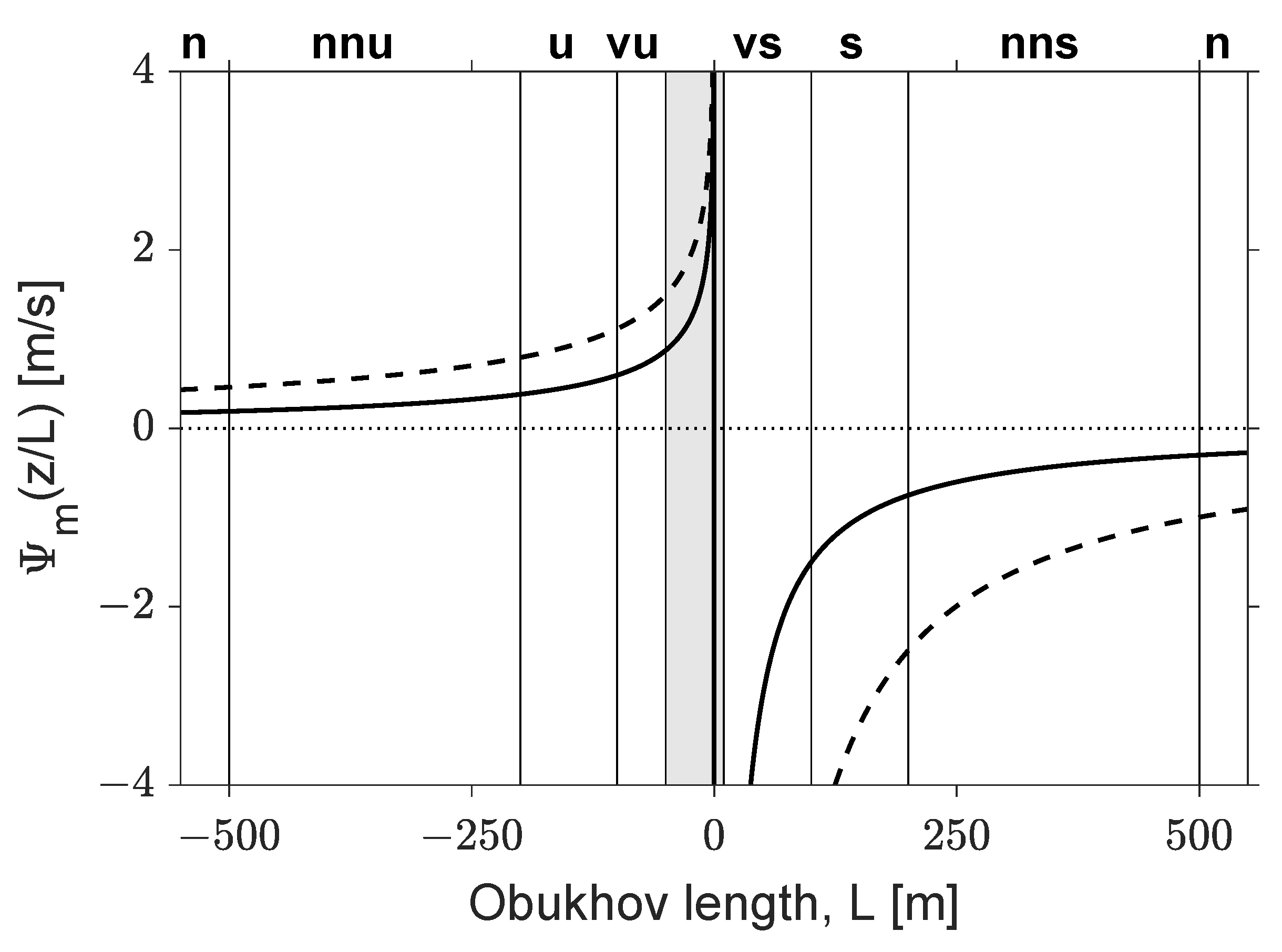
3.2. Surface-Layer theory

The vertical wind gradient for a neutral, homogeneous, and stationary flow can expressed as [41]
U z = u * l ,
where u * is the friction velocity and l is the mixing length [42]. In the surface layer, which corresponds to the lowest 5–10% of the boundary layer, the magnitudes of stress and turbulent fluxes generally vary by less than 10% with height [43]. Thus, within the surface layer, two assumptions are commonly made: (i) the friction velocity variation with height is negligible, and (ii) the mixing length increases with height as l ( z ) = κ z [44], where κ 0.4 is the von Kármán constant. The logarithmic wind profile for neutral atmospheric conditions is the integral of Equation (1):
U ( z ) = u * k ln z z 0 ,
where z 0 is the roughness length, which is the height at which the mean wind speed becomes zero. Over sea, the roughness length is commonly expressed using the Charnock’s relation,
z 0 = α c u * 2 g ,
where g = 9.81 m/s 2 is the gravitational acceleration and α c is the Charnock’s parameter, α c 0.012 [45].
According to MOST, the influence of atmospheric stability over the wind speed gradient within the surface layer is expressed by the dimensionless wind shear, ϕ m , as
U z = ϕ m u * κ z .
The dimensionless wind shear takes different functional forms depending on the atmospheric stability conditions. It is usually described by the experiment-based Businger–Dyer functions ([46,47]):
ϕ m = 1 + β z L , f o r z L > 0 ( stable ) 1 , f o r z L = 0 ( neutral ) 1 γ z L 1 4 , f o r z L < 0 ( unstable ) ,
where L is the Obukhov length, z L is the dimensionless stability parameter, and β = 6.0 and γ = 19.3 are empirical constants [48], later validated by Holtstag et al. [33] for the IJmuiden site.
Thus, under non-neutral conditions the diabatic wind profile can be expressed as
U ( z ) = u * κ ln z z 0 Ψ m z L ,
where Ψ m z L is the stability correction function [32,43]
Ψ m z L = β z L z L > 0 ( stable ) 0 z L = 0 ( neutral ) 2 ln ( 1 + x 2 ) + ln ( 1 + x 2 2 ) 2 arctan ( x ) + π 2 z L < 0 ( unstable ) ,
where x = 1 γ z L 1 / 4 . Although the Businger–Dyer functions were empirically derived from data collected over land, their applicability has been successfully tested and validated for the estimation of the offshore wind profile [33,49].
The Obukhov length can be used to classify atmospheric stability conditions, classified into stable ( L > 0 ), neutral ( L ± ), or unstable ( L < 0 ). With a view to Section 4 two atmospheric stability classifications are listed in Table 2 and Table 3 according to the definition classes for L of van Wijk et al. [50] and Gryning et al. [51].
The behavior of the stability correction Ψ m z L as a function of the Obukhov length L is depicted in Figure 2.
Finally, we introduce the wind-speed ratio between HWSs at two heights, z 1 and z 2 , z 2 > z 1 , is therefore,
W S R ( z 1 , z 2 , L ) = U ( z 2 ) U ( z 1 ) = ln z 2 z 0 Ψ m z 2 L ln z 1 z 0 Ψ m z 1 L .
The wind-speed ratio is a proxy of wind shear that will be used to analyze the dependence of wind shear on the dimensionless stability, z L , further.

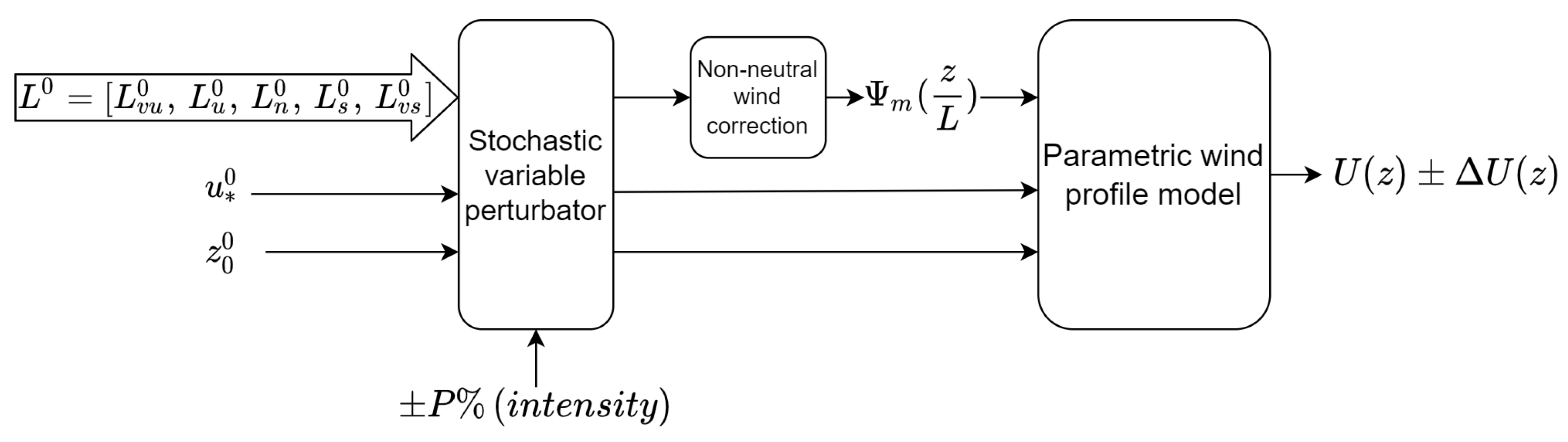
3.3. Parametric Wind Model Estimation

We estimate atmospheric stability based on FDWL HWS profiles measured at a discrete number of heights. We propose solving Equations (6) and (7) for model variables L, u * , and z 0 . The algorithm’s sensitivity to these three variables and consequent dimensionality reduction of the problem (two-variable problem, L and u * ) is provided in Section 4.2.
The optimization problem can be formulated as
( L , u * , z 0 ) = a r g m i n L , u * , z 0 | | U F D W L U ( z , L , u * , z 0 ) | | 2 ,
where the function U ( z , L , u * , z 0 ) is the parametric wind profile model formulated by Equation (6) and piece-wise by Equation (7). Below, functions are assimilated into vectors and treated indistinctly. A constrained nonlinear least squares (NLSQ) method is used to solve the model parameters, L, u * , and z 0 , minimizing the error norm between the model vector, U ( z ) , and the FDWL-measurement vector, U F D W L .
The diabatic correction function Ψ m ( z L ) (Equation (7), Figure 2) becomes ill-posed for Obukhov lengths close to zero ( L = 0 ) and exhibits a nearly flat behavior for large values of the Obukhov length ( | L | ). Additionally, Ψ m ( z L ) is a piece-wise function. To facilitate NLSQ convergence, we define upper and lower search bounds for each of the parameters to be optimized as
  • L [ 2000 , 1 ] [ 1 , 2000 ] m,
  • u * [ 0 , 1.4] m/s, and
  • z 0 [ 10 5 , 10 2 ] m.
The limiting bounds for the roughness length z 0 in offshore environments follow [43,52]. The friction velocity bounds are in agreement with those found in different experimental campaigns in the literature [53,54] and represent roughly a factor 1.5 over the range of practical friction velocities retrieved by the sonic anemometers (Section 3.5, Equation (14)). The search bounds for the Obukhov length, L, are, e.g., a factor two and four over the practical neutral stability thresholds given by Van Wijk et al. [50] (Table 2) and Gryning et al. [51] (Table 3), respectively. Larger values do not tend to substantially improve the algorithm search performance (see Section 4.2).
Optimization starting vector. Two start points, one positive, L + [ 1 , 2000 ] , and one negative, L [ 2000 , 1 ] , are set to L + = 500 m and L = 500 m, respectively, as initial guesses for the Obukhov length. This allows us to avoid the asymptotic discontinuity of Ψ m ( z L ) at L = 0 (Figure 2). The initial guesses for the friction velocity, u * , and roughness length, z 0 , are set to 0.7 m/s and 5e-3 m, respectively, which are the mean values of these variables in the above search ranges. From these two starting vectors, ( L + , u * , z 0 ) and ( L , u * , z 0 ) , a positive and a negative search is started by the NLSQ algorithm and two candidate solution vectors are obtained. The vector with the smallest error norm is chosen as the solution.

3.4. Reference Measurements: Atmospheric Stability

Reference metmast-derived Obukhov length and friction velocity are needed in order to assess the performance of the proposed algorithm in Section 3.3 above. In the present and following subsection (Section 3.5), different methods to estimate such reference parameters are presented.
Conventionally, the Obukhov length is directly computed from turbulence fluxes measured (from wind and temperature observations at similar heights), e.g., with a sonic anemometer [43]. However, the sonic anemometer at 85 m available only recorded velocity observations. Alternatively, the method by Grachev and Fairall [55] to estimate the Obukhov length, L, provides a way out when air and sea temperature observations are available, as is the case. They found empirical dependency between the bulk-Richardson number, R i , and the dimensionless stability parameter. Their method has been used in recent studies [33,56].
The bulk Richardson number is an approximation of the gradient Richardson number in which actual local gradients in an atmospheric layer are approximately computed by measurements at a couple (or a series of) discrete heights. The bulk Richardson number is defined as [43]
R i = g Δ θ ¯ v Δ z θ ¯ v U 2 , z [ z b o t t o m , z t o p ] ,
where Δ θ ¯ v = θ ¯ v ( z t o p ) θ ¯ v ( z b o t t o m ) is the difference between the mean virtual potential temperature at the top layer height, z t o p , and bottom layer height, z b o t t o m and Δ z = z t o p z b o t t o m . Here, z t o p = 21 m above LAT and z b o t t o m = 0 m above LAT. θ ¯ v is the mean potential temperature in the layer and U is the mean wind observed at z t o p (at this point we note that U is formally defined as Δ U = U ( z t o p ) U ( z b o t t o m ) = U ( z t o p ) on account of the fact that U ( z b o t t o m ) = 0 ). In practice, U is the 10 min averaged wind observed at 27 m.
The potential temperature is estimated from the expression [43,57]
θ v ( z ) = T ( z ) P 0 P ( z ) R / C p 1 + 0.61r ( z ) ,
where T (K) is the temperature, P 0 = 1000 hPa is the reference pressure, P is the air pressure, R 287 J/(K·kg) is the gas constant of air, C p 1004 J/(K·kg) is the specific heat capacity at a constant pressure for air, and r is the mixing ratio (unsaturated air).
In this study, we computed the mean potential temperature θ ¯ v at 21 m from the mast temperature, pressure, and humidity data at 21 m. θ ¯ v at sea-level was computed from the wave-buoy-measured 60 min mean water temperature [58], which was interpolated down to 10 min resolution, according to wind-energy standards [11]. The pressure and relative humidity at sea level were calculated by extrapolating the mast pressure and humidity vertical profiles from the sensors at 21 m and 90 m (Figure 1) down to 0 m. Pressure and relative humidity at 0 m as well as water-temperature at 10 min resolution were computed via shape-preserving piecewise cubic interpolation [59,60].
Subsequent to the calculation of R i , the dimensionless stability parameter ζ = z / L is computed as
ζ = 10 R i R i 0 10 R i 1 5 R i 0 < R i < 0.2 .
The constants 10 and 5 above are empirical values [55]. The latter implies a critical stable R i of 0.2 so the theory has a limitation when the conditions are very stable. Besides, when using the bulk Richarson number approximation, the thicker the layer, the more likely to smooth out large gradients in the layer and, therefore, to misestimate the occurrence of turbulence [43].
When we derive L from Equation (12) we refer to it as L R i ,
L R i ( z ) = z ζ ,
where z is a reference height ensuring the validity of the bulk Richardson model (Equation (10)) above in the layer [ z b o t t o m , z t o p ] . In the standard methodology ([55]), z is taken as the sonic-anemometer observational height (11 m). However, in the case of IJmuiden, temperature and particularly the wind-speed observational heights are relatively high, 21 and 27 m, respectively. Although a rough estimation of the reference height can simply be taken as the mean height between the air observational height and sea level [33], in this case, z ( z t o p + z b o t t o m ) / 2 = 10.5 m, accurate estimation of the reference height is more involved.
In order to estimate the most accurate meaningful reference height, z , the following procedure was carried out: different estimations of L R i ( z ) were retrieved from Equation (13) by varying z from the layer top observational height ( z t o p = 21 m) to the rough reference height (10.5 m) in steps of 0.5 m, i.e., z = 21 , 20.5, , 10.5 m. As a result, we obtained 22 different sets of L R i ( z ) values, each one corresponding to a z . Next, the MOST model wind-speed ratio of Equation (8) was computed for all sets of the L R i ( z ) as well as the coefficient of determination, ρ 2 , between the measured and modeled wind-speed ratios. The z (equivalently, L R i ( z ) ) with the highest ρ 2 yielded the sought-after reference height. Thereby, z = 15.5 m was found to be the reference height ensuring the highest ρ 2 after the outlier screenings applied over L R i ( z ) and the measured wind-speed ratio (see the outlier screening and the results in Section 4.3).

3.5. Reference Measurements: Friction Velocity

The friction velocity is a form by which a shear stress may be rewritten in units of velocity such as the velocity that relates wind shear between layers of flow, e.g., for neutral condition u * = κ · ( U ( z 2 ) U ( z 1 ) ) / l n ( z 2 / z 1 ) (Equation (2)). Two reference methods are considered for comparison:
The first solves Equation (6) for u * given the Obukhov length L R i estimated from the bulk Richardson number using Equation (13) and mast HWS measurements at 27 m. The roughness length z 0 is computed from Equation (3). This method can be viewed as "mast" 1D ( u * 1 D ).
The second uses directly the measured turbulent fluxes [43],
u * s o n i c = u w ¯ 2 + v w ¯ 2 0.25 .
For these computations, we used the sonic measurements at 85 m.

3.6. Data Screening

To begin with, FDWL, mast-sensors and mast-DWL data were averaged to a common uniform time resolution of 10 min, which is according to WE standards [11]. Accordingly, the wave-buoy-derived water temperature was resampled from 60 to 10 min as already mentioned in Section 3.4.
Regarding anemometers’ data, the screening procedure relied on selection of the true wind direction (TWD) [40]. To do this, WD and HWS measurements from all the three anemometers at each of the three metmast measurement heights (27, 58.5 and 85 m) were checked. Figure 3 sketches a top-view of mast depicting the positions of the wind vanes and anemometers at each height. First, the middle WD (MWD) was computed as the median of the WD measurements by the three anemometers. Then, the TWD was derived following these criteria (see Figure 3a):
  • If the MWD lay on the red crown, the TWD was computed as the mean WD between vanes HxxB240 and HxxB120,
  • If (…) on the blue crown, (…) between vanes HxxB0 and HxxB120, and
  • If (…) on the green crown, (…) between vanes HxxB240 and HxxB0.
Finally, the true wind speed was chosen as the one retrieved from the anemometer over which the TWD was within a confidence angle range (the wake-free range) of 90 ± 30 (Figure 3b) in relation its boom orientation.
Concerning the lidar instruments, HWS measurements lower than 2 m/s or higher than 100 m/s were rejected on account of the ZephIR-300 manufacturer’s specifications [22]. Regarding the FDWL, it is well-known that motion-induced effects on the retrieved wind vector become prominent at a 1-s temporal resolution but are negligible at the 10 min level. For the latter case, motion effects increase fluctuations on the wind speed [21,39,61]. At the 10 min level, it was shown [62,63] that the spatial variation (SV) parameter (see below) can be used as a threshold to filter data as it represents a trade-off between key performance indicator (KPI) improvements and data availability.
FDWL measurement outliers were identified by plotting the HWS differences between the metmast and FDWL measurements as a function of different FDWL internal parameters, namely, the backscatter, bearing (compass), points in fit out of the 50 radial velocities within a full scan (see below), SV, precipitation, and visibility. For each internal parameter, we considered as outliers the samples which yielded differences higher than 2 m/s in relation to metmast reference. The same analysis was conducted with the mast-DWL, which served as the reference lidar.
Backscatter refers to the intensity of the Doppler lidar echo. Bearing refers to the lidar pointing direction with respect to the Earth’s magnetic North. Points in fit and SV are parameters related to the Velocity Azimuth Display (VAD) algorithm used by the lidar to retrieve the wind vector under the assumption of uniform wind. The SV is an indicator of the goodness of the VAD fitting of the radial velocities within the lidar scanning circle used to retrieve the wind vector at a given height. Therefore, the SV can be understood as a turbulence parameter describing the variation degree of the radial wind speeds within the scan [64]. High SV values are associated to measurements for which the hypothesis of uniform wind during the lidar scan is no longer valid [39]. This leads to outlier measurements, which must be removed.
Numerical analysis showed that the largest differences in HWS between the mast anemometer and FDWL measurements were attributable to bearing and SV of the FDWL. Therefore, we applied the following outlier rejection criteria:
(i)
HWS < 2 m/s or HWS > 70 m/s,
(ii)
bearing = 0 (FDWL compass issue, see Section 4.1), and
(iii)
95th percentile spatial-variation threshold.

4. Results and Discussion

4.1. Data Screening and Quality Assurance

Now, we discuss our results for outlier criteria (ii) and (iii) which were introduced in Section 3.6 above. Figure 4a shows the HWS difference between the cup anemometer and the FDWL measurements at 83 m as a function of the FWDL bearing. Similar results were found for the two other FDWL heights, 25 and 56 m (not shown). Figure 4b shows a similar plot but for the mast-DWL. As expected, the FWDL bearing covers the full range of motion, whereas the mast-DWL bearing remains mostly fixed at 3 . The largest HWS differences occur for bearings equal to zero, which lacks physical consistency and might show an issue in the data acquisition system.
Figure 5 shows the histogram of SV from the FDWL at 25 m and the HWS differences as a function of the SV between the 27-m cup anemometers and the FDWL, respectively. In Figure 5a, the border line between the white and grey shades delimits the 95th percentile of the one-tailed spatial-variation distribution. This percentile corresponds to a SV threshold, SV = 0.055 and SV 0.055 0.065 for the other measurement heights of the lidar (data not show). For the mast-DWL, the 95th percentile corresponds to the threshold SV 0.07 (data not shown). The SV thresholds used here for 10 min data were found to be more conservative than those used in previous studies (SV 0.1 ) [62,63], in which the FDWL measurements were compared against metmast values for quality assurance (QA).
The appropriateness of the SV filtering criterion is re-encountered in Figure 5b, which shows that HWS differences between the FDWL and the metmast measurements started to deviate from the ideal 0-m/s bias (dashed red line) for SVs above approximately 0.05, which justifies our choice for criterion (iii) in Section 3.6.
Regarding the anemometers, Figure 6 shows the HWS differences between the cup anemometers and the lidars as a function of direction. The reduction on the scattering of data after application of the TWD screening criterion is well noticed (black versus grey dots). Quantitatively, after outlier rejection, peak HWS differences were below ±1 m/s at all heights, which shows that the mast effects were effectively removed.
The 82-day IJmuiden campaign produced a dataset with 10,833 10 min samples. After the filtering procedure described in Section 3.6, we obtained 8263 10 min samples. Figure 7 shows that both the cup anemometers and the fixed and floating lidars measured very closed HWSs with determination coefficients higher than ρ 2 = 0.996 and slopes of the regression lines between 0.985 and 1.010 at all measurement heights, as expected from previous studies [17,18,19,20,21]. These values are within the KPIs defined by the Carbon Trust’s Offshore Wind Accelerator (OWA) [4].

4.2. Sensitivity to the Wind Model Parameters

In order to analyze the sensitivity of the parametric wind model presented in Section 3.2 with respect to Equation (9) model parameters, a sensitivity simulator was implemented (Figure 8). The simulator inputs are the model parameters Obukhov length L, friction velocity u * , and roughness length z 0 , denoted as L 0 , u * 0 , and z 0 0 , respectively. These inputs were perturbed by an intensity factor ± P % ( ± 10%). Then, the perturbed inputs were used to compute the non-neutral wind correction Ψ m z L using Equation (7). Finally, the perturbed wind profile, U ( z ) + Δ U ( z ) , was simulated as a function of the perturbation intensity on the input variables through Equation (6). Five different atmospheric stability scenarios were considered: very unstable, unstable, neutral, stable, and very stable, based on Obukhov length values denoted by L v u 0 , L u 0 , L n 0 , L s 0 , and L v s 0 , respectively.
The error propagated on the model wind profile was found to be insensitive to perturbations in the roughness length z 0 . Therefore, practical implementation of the algorithm embeds Equation (3) into Equation (6) as
U ( z ) = u * κ ln z α c u * 2 g Ψ m z L ,
Thus, the model dimension reduces from three (L, u * , and z 0 ) to two (L and u * ), hereafter called the 2D algorithm. Likewise, slight deviations in the Charnock’s constant (Equation (3)) have low impact on the retrieved wind model parameters (L and u * ). Furthermore, as expected from correction function Ψ m ( z L ) (Figure 2), the sensitivity of the model wind profile with respect to the Obukhov length was found to be proportional to 1 / | L | . Further discussion is given in Section 4.4, in line with the statistical results encountered.

4.3. Wind Shear Dependence on Dimensionless Stability

The dependence of the wind speed ratio (Equation (8)) on the dimensionless stability computed from both the 2D Obukhov length ( z L ^ ) and from the Ri reference ( z L R i ) enabled us to quantify the performance of the 2D algorithm. The wind speed ratio was computed between the top and bottom measurement heights of both the FDWL (83 m and 25 m) and the mast (85 m and 27 m). As described in Section 3.4, z = 15.5 m was taken as the reference height. We used 8,263 10 min clean data records (Section 3.6). Additionally, two successive levels of outlier filtering were considered: (i) retrieved Obukhov lengths in the interval ( 50 < L R i < 10 ) m were rejected because these values were outside the stability limits in Table 3, and (ii) wind speed ratios were histogram-filtered. To achieve the latter, the dimensionless stability range was divided into 0.01-width bins and, in each bin, the wind-speed ratios outside of the μ ± 1 σ (with μ being the mean and σ being the standard deviation of the wind-speed ratio distribution in the bin) were rejected as outliers.
Figure 9a,b plots FDWL and metmast wind-speed ratios as a function of dimensionless stability parameter z L ^ , respectively. Figure 9c plots metmast wind-speed ratio as function of z L R i .
The FDWL wind-speed ratio as a function of z L ^ (Figure 9a) yielded the best statistical indicators either if all or nonoutlier samples were considered ( ρ a l l 2 = 0.965 , R M S E a l l = 0.029 ; ρ 1 σ 2 = 0.988 , R M S E 1 σ = 0.016 , respectively). This was expected because the FDWL-derived HWSs were used to retrieve the estimated Obukhov length L ^ using the 2D method, which, in turn, relies on the Businger–Dyer functions. Figure 9b provides tiebreaker proof confirming the successful performance of the 2D algorithm. Thus, in Figure 9b, the mast-derived wind speed ratios are compared to the estimated L ^ values, and the statistical indicators found ( ρ 1 σ 2 = 0.974 and R M S E 1 σ = 0.023 ) are virtually coincident with those in Figure 9a. Additionally, when comparing the distribution of the points along the horizontal axes in Figure 9b,c ( z L ^ and z L R i , respectively), figures that share identical mast data, the spread along the z L ^ axis (2D algorithm) is narrower than along the z L R i (Richardson reference). Again, this confirms the superior performance of the 2D algorithm. Regarding Figure 9c, and despite the clear dependence obtained between the wind-speed ratio and dimensionless stability z L R i , the huge number of outliers suggests that not all measured wind profiles were acceptably modeled by the MOST model (Equation (6)).
In non-MOST situations, e.g., low-level jet and storm events, the estimates of the 2D-algorithm may be highly biased. The residual norm between the measured and fitted wind profiles has been used to quantitatively assess the 2D-algorithm accuracy. The residual norm is indicative of the quality of the fitting and is defined as the norm of the error between the parametric and the measured wind profiles. Most of the records showed residual norm values between 0 m/s and 2.21 m/s. Occurrences with a residual norm higher than the residual norm 95th percentile, corresponding to a value of 0.42 m/s, were filtered out (413 records). In the vast majority of cases, the 2D-algorithm is able to converge because most of experimental wind profiles measured by the FDWL are well predicted by MOST.

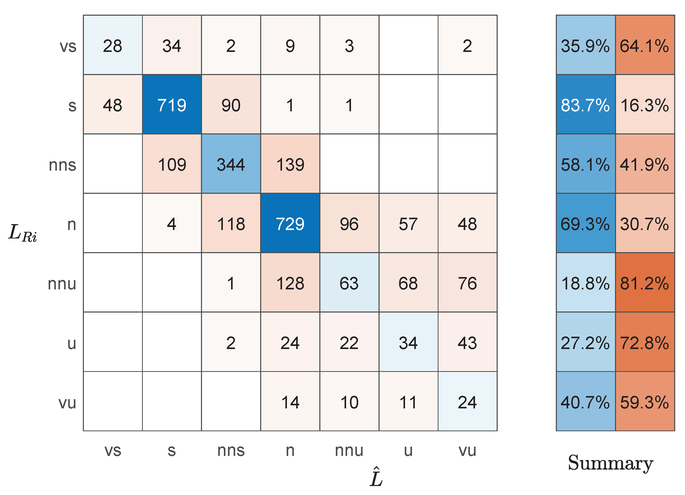
4.4. Performance Statistics: Friction Velocity and Stability

The performance of the 2D algorithm with regard to friction velocity u * was assessed by comparing the velocity estimated using the 2D algorithm, u ^ * with the two reference velocities described in Section 3.5, namely, the reference u * s o n i c computed by the sonic anemometer and the mast-derived u * 1 D computed by the 1D method (Figure 10).
Figure 10a shows that the points ( u * s o n i c , u ^ * ) were scattered widely. This was further corroborated by numerical analysis, which yielded a linear regression (LR) u ^ * = 0.813 · u * s o n i c + 0.113 , coefficient of determination ρ 2 = 0.731 , and R M S E = 0.077 m/s. These comparatively modest indicators are due to the fact that the sonic anemometer was located at a height of 85 m, which may well be beyond the surface layer. Above the surface layer, the proposed model is not valid, which leads to biased estimations [43]. Worse results were attained when considering alternative values for Charnock’s parameter, α c , which is a site-dependent parameter here assumed as α c = 0.012 based on previous studies [33,44,65,66]
When comparing u ^ * against mast-derived u * 1 D (Figure 10b), a much better agreement is found. This is supported by a LR as good as u ^ * = 0.965 · u * 1 D + 0.022 , which is virtually the ideal 1:1 line; ρ 2 = 0.956 ; and R M S E = 0.031 m/s.
The performance of the 2D algorithm for the estimated Obukhov length, L ^ , was tested against the Richardson reference, L R i , for the whole campaign. For this task, two well-accepted stability classification criteria in the literature were considered: (i) Van Wijk’s (Table 2), and (ii) Gryning’s criteria (Table 3).
Van Wijk’s classification.Figure 11 compares classification results among the Obukhov lengths estimated by the 2D algorithm, L ^ , and by the Ri estimate, L R i . The type criteria are provided in Table 2. Figure 11a,b shows similar but not identical results. For example, the hourly evolution of the stable and neutral classes is nearly identical for both estimators. However, this is not the case for very unstable class, which was overestimated by the 2D algorithm to the detriment of the unstable class when compared to the Richardson reference. Similar results can be derived from Figure 11c,d. Thus, the 2D method yielded 33% of very unstable cases, whereas the Richardson reference yielded 25%.
Gryning’s classification. A similar analysis was conducted for the Gryning classification (Table 3). This criterion essentially breaks down the Van Wijk stability classes into subclasses in order to create room for the near-neutral stable and near-neutral unstable subclasses.
Figure 12 compares the classification results yielded by the 2D algorithm, L ^ , and Ri estimate, L R i . Figure 12a,b shows similar temporal behavior for the very stable and stable classes over the course of the day. The latter class became prominent during the last hours of the day. In contrast, as occurred with the Van Wijk classification, the neutral class and all the unstable classes estimated by the 2D algorithm exhibited larger variations compared to the Richardson reference. When comparing L ^ to L R i in the pie charts, 5% ( L ^ chart) vs. 3% ( L R i chart) of the cases were classified as very unstable, 11% vs. 15% were classified as unstable or near-neutral unstable. In contrast, the following classes remained essentially the same: 31% ( L ^ panel) vs. 31% ( L R i panel) for the neutral case, 19% vs. 19 % for the near-neutral stable case, 28% vs. 27% for the stable case, and 4% vs 4% for the very stable class.
Next, we quantified classification performance by rating the one-to-one stability class correspondence between L ^ and L R i . This one-to-one correspondence is expressed via a confusion matrix, in which each matrix row represents the instances in an actual reference stability class ( L R i ), and each column represents the instances in an estimated stability class ( L ^ ). Figure 13 depict the matrix obtained when considering the Gryning classification criterion. An ideal predictive method would have all instances along the main diagonal of the confusion matrix. Thus, bluish cells represent instances in which the estimated stability class matches the Richardson reference class, whereas reddish cells represent misclassifications. In order to quantitatively assess performance of the 2D algorithm, we define the hit rate (HR) as
H R [ % ] = no . of correct estimations no . of estimations × 100 .
The miss rate is simply the complementary function 1 H R . Figure 13 depicts the confusion matrix considering Gryning’s stability classes (Table 3). We found that the estimated classes lay along a band formed by the main diagonal, the first diagonal below this, and the first diagonal above the main diagonal. Thus, an overall HR of 62.59% was obtained and the remaining 29.21% corresponded to the classes estimated by the 2D algorithm that were adjacent to the correct ones given by the Richardson reference. The summary matrix shows a very high miss rate in unstable atmospheres with the HRs ranging from 18.8% to 40.7%. The low HRs attained for the nnu, u, and vu classes occurred due to the low sensitivity of the wind shear model in Equation (6) with respect to the Obukhov length for unstable atmospheres. This is re-encountered in Figure 14a, in which the median wind profiles and related 25th to 75th percentiles are plotted parameterized by stability condition. For the nnu, u, and vu classes, the percentile bars overlap (dark green, red, and magenta traces, respectively), which makes it impossible for the 2D algorithm to discern them.
In contrast, “s”, “nns”, and “n” classes scored HRs of 83.7%, 58.1%, and 69.3%, respectively, on account of their higher sensitivity, which, in turn, led to higher discernability among these classes. It is also worth noting the low HR (35.9%) achieved by the “vs” class. One reason accounting for that is the comparatively short span of Obukhov lengths included in the “vs” class ( 10 L < 50 ) in Table 3. This was a too short span for the NSLQ solver to estimate the Obukhov length at such fine level of accuracy, which eventually led to miss-classification between the “vs” and “s” classes. This is also evidenced in Figure 14a by overlapping percentile bars for these classes.
Analogously to Figure 13, Figure 15 represents the confusion matrix considering the Van Wijk stability classes (Table 2). An overall HR of 66.07% and a misclassification rate of 33.93% were observed. The estimation performance varied widely, ranging from HRs of 26.2% for the u class to 88.3% for the vs class. Again, the low HRs were due to the low sensitivity of the wind shear model with respect to the Obukhov length in unstable conditions, as evidenced in Figure 14b.
By comparing Figure 15 and Figure 13 (equivalently, Figure 11 and Figure 12) Van Wijk’s classification criterion shows better performance than Gryning’s. Although both have similar HRs (66.07% for Van Wijk and 62.59% for Gryning), the Van Wijk confusion matrix (Figure 15a) scores higher HRs than Gryning’s in all but the u class, as indicated by the reddish cell in the summary matrix. This, however, warrants some comments. For example, the good match between the estimated and reference stability classes in the pie chart in Figure 12 for the Gryning classification hides a population inversion between the right- and left-adjacent classes to the main diagonal (Figure 13). This also applies to Figure 15a. Experiments also showed that wind profiles often became indistinctly misclassified into adjacent classes, as shown by the overlapping error bars in Figure 14. A method to mitigate this issue involves collapsing all unstable subclasses into an aggregated class named "unstable". Specifically, this aggregation leads to vs, s, n, and u classes in the Van Wijk classification (Figure 15b), and to vs, s, nns, n, and u classes in Gryning’s classification (figure not shown). As a result, a much better agreement between the estimated and reference stability classes was achieved, as indicated by the higher HRs attained in all classes. Quantitatively, the overall HR increased to 73.6% for the Van Wijk classification. Similar results were achieved for the Gryning classification (figure not shown), which scored an HR of 72.6%.
It is important to mention that although we use L R i as the reference, it cannot be considered as the ground-truth reference for one-to-one comparison with L ^ , because it was not derived exactly as proposed by Grachev et al. [55] due to the absence of turbulent fluxes measurements in the surface layer and the different instrumental measurement heights available. However, it is a good indicative of the method goodness in terms of atmospheric classification. In order to validate the method against a third party, the stability estimated by the 2D-algorithm was compared against the stability estimated by means of virtual potential temperature gradient ( d θ v / d z ) between 90 and 21 m. Virtual potential temperature was retrieved using temperature, pressure and relative humidity data from the IJmuiden mast via Equation (11). The potential temperature gradient indicator is only able to discern between two stability classes: unstable ( d θ v / d z < 0 ) and stable ( d θ v / d z > 0 ). Considering these categories, HRs higher than 82% were found for the comparison between L ^ and d θ v / d z , further proving the goodness of the 2D algorithm.

5. Summary and Conclusions

In this study, we suggested an 2D algorithm that accurately estimated both the Obukhov length and the friction velocity, hence, correctly determined atmospheric stability from FDWL measurements at four different heights. We used the spatial variation within the lidar scans as an important filtering parameter of the FDWL (Figure 5). The parameter is a proxy of turbulence; high spatial variation is associated to nonuniform wind during the scan. The latter can originate either from apparent turbulence (i.e., induced by sea motion) or from true wind turbulence [62]. When comparing FDWL to mast-based wind speeds, we found that the mean winds were biased less than 1.5% (LR, U F D W L = 0.985 · U m a s t + 0.018 ) with a determination coefficient, ρ 2 = 0.996 , and a RMSE as low as 0.25 m/s. Similar values were found for the fixed DWL on the mast.
The algorithm assumes that the measured FDWL wind profiles follow MOST and the Charnock’s relation is used to parameterize the roughness length. Over the sea, with such low roughness, the sensitivity of the roughness on the estimated parameters can be neglected. A parametric sensitivity study showed that unstable wind profiles exhibited lower sensitivity than stable wind profiles to variations of the Obukhov length (Figure 14).
The 2D-estimated Obukhov length and friction velocity were compared with reference to the mast-derived Obukhov length using the Richardson number, to the sonic-anemometer-derived friction velocity, and the 1D-model-derived friction velocity. Thus, the 2D-estimated friction velocity was largely in agreement with the sonic-anemometer-derived and the 1D-model-derived friction velocities, with coefficients of determination of 0.72 and 0.94 , respectively (Figure 10).
We also examined the performance of the algorithm by classifying atmospheric stability in a number of classes. When comparing the relative frequencies of occurrence of each class of the Van Wijk classification, differences occurred between 0% and 10% (Figure 11) and between 0% and 4% for Gryning’s classification (Figure 12). Notwithstanding these results, analysis through confusion matrices showed HRs of 65.24% for the Van Wijk and 62.63% for the Gryning classification. Higher HRs were attained for stable regimes than for unstable ones due to the lower sensitivity of the 2D algorithm to the Obukhov length in unstable regimes. This issue was addressed by collapsing the unstable sub-classes into a unique aggregated class named "unstable". For the Van Wijk’s, this reclassification improved the HR up to 72.9% and up to 72.4% for the Gryning’s. The confusion matrix study also showed that although simple pie chart statistics (Figure 12) indicate a very good one-to-one correspondence between the estimated stability class (through L ^ ) and the Richardson reference class (through L R i ), this correspondence is only apparent because cross-correspondences occur frequently between classes adjacent to the main diagonal (Figure 13 and Figure 15). This effect became more prominent for classes falling in an Obukhov length interval in which Businger–Dyer’s correction function had a flatter derivative (i.e., less gradient). Other misclassifications were attributable to anomalous profiles such as those associated with low-level jets. Moreover, the bulk Richardson number methodology used to compute the gradient Richardson number is just a two-point approximation of the derivative of the local wind and temperature gradients in the surface layer. Finally, the performance of the algorithm in terms of stability classification was compared against the virtual potential temperature gradient method acting as a proxy of stability. HRs higher than 82% were encountered, further validating the algorithm performance.
Overall, we aimed to show the potential of FDWLs for offshore wind resource assessment as a standalone instrument and the ability of an algorithm to estimate atmospheric stability from the FDWL wind speeds only. As further steps, we would like to evaluate the algorithm’s performance against direct measurements of both momentum and heat fluxes taken over the same range of heights. Additionally, a comparison between the 2D-algorithm and other methods based on MOST relationships is still required.

Author Contributions

This work was developed as part of M.P.A.d.S.’s doctoral thesis supervised by F.R.; 2D optimization algorithm methodology, F.R. and M.P.A.d.S.; software development, J.F.-G., A.S.-B. and M.P.A.d.S.; analysis and figures, M.P.A.d.S. and A.S.-B.; writing—original draft preparation, M.P.A.d.S. and A.S.-B.; review and editing, F.R. and A.P.; funding acquisition, F.R.; conceptualization support, F.R. and A.P.; measurement campaign lead, D.G.-M. All authors have read and agreed to the published version of the manuscript.

Funding

This research was part of the projects PGC2018-094132-B-I00 and MDM-2016-0600 (CommSensLab Excellence Unit) funded by the Ministerio de Ciencia e Investigación (MCIN)/Agencia Estatal de Investigación (AEI)/10.13039/501100011033/ FEDER. The work of M.P.A.S was supported under grant PRE2018-086054 funded by MCIN/AEU/10.13039/501100011033 and FSE “El FSE invierte en tu futuro”. The work of A.S-B was supported by grant 2020 FISDU 00455 funded by Generalitat de Catalunya—AGAUR. The European Commission collaborated under projects H2020 ACTRIS-IMP (GA-871115) and H2020 ATMO-ACCESS (GA-101008004). The European Institute of Innovation and Technology (EIT), KIC InnoEnergy project NEPTUNE (call FP7), supported the measurement campaigns.

Institutional Review Board Statement

Not applicable.

Informed Consent Statement

Not applicable.

Data Availability Statement

The data presented in this study are available upon request from the corresponding author, roca@tsc.upc.edu.

Acknowledgments

A. Peña and J. Mann (Denmark Technical University, DTU) are gratefully acknowledged for hosting M. P. Araújo da Silva and A. Salcedo-Bosch during their Ph.D. secondments to DTU. I. Karagali (Danish Meteorological Institute) is kindly acknowledged for her technical assistance.

Conflicts of Interest

The authors declare no conflict of interest.

Abbreviations

The following abbreviations are used in this manuscript:
DWLDoppler Wind lidar
FDWLFloating Doppler Wind lidar
HRHit Rate
KPIKey Performance Indicator
HWSHorizontal Wind Speed
LATLowest Astronomical Tide
LoSLine of Sight
LRLinear Regression
metmastMeteorological Mast
MOSTMonin-Obukhov Similarity Theory
NLSQNon-Linear Least Squares
OWEZOffshore Wind Farm Egmond aan Zee
RMSERoot-Mean-Squared Error
TWDTrue-Wind Direction
VADVelocity Azimuth Display
WDWind Direction
WEWind Energy

References

  1. Council, G.W.E. Global Wind Report 2018; Technical Report; Global Wind Energy Council: Brussels, Belgium, 2019. [Google Scholar]
  2. Gutiérrez Antuñano, M. Doppler Wind LIDAR Systems Data Processing and Applications: An Overview towards Developing the New Generation of Wind Remote Sensing Sensors for Offshore wind Farms. Ph.D. Thesis, Universitat Politècnica de Catalunya, Barcelona, Spain, 2019. [Google Scholar]
  3. Global Wind Energy Council. Global Wind Energy Outlook 2016; Technical Report; Global Wind Energy Council: Brussels, Belgium, 2016. [Google Scholar]
  4. Carbon-Trust. Offshore Wind Accelerator Roadmap for the Commercial Acceptance of Floating LIDAR Technology; Technical Report; Carbon Trust: London, UK, 2018. [Google Scholar]
  5. Hevia-Koch, P.; Jacobsen, H. Comparing offshore and onshore wind development considering acceptance costs. Energy Policy 2019, 125, 9–19. [Google Scholar] [CrossRef]
  6. IRENA. Future of Wind: Deployment, Investment, Technology, Grid Integration and Socio-Economic Aspects; Technical Report; International Renewable Energy Agency: Abu Dhabi, United Arab Emirates, 2019. [Google Scholar]
  7. Sathe, A.; Mann, J. A review of turbulence measurements using ground-based wind lidars. Atmos. Meas. Tech. 2013, 6, 3147–3167. [Google Scholar] [CrossRef] [Green Version]
  8. WindPower. Do We Still Need Met Masts? 2018. Available online: https://www.windpowermonthly.com/article/1458018/need-met-masts (accessed on 6 April 2021).
  9. Gottschall, J.; Wolken-Möhlmann, G.; Lange, B. About offshore resource assessment with floating lidars with special respect to turbulence and extreme events. J. Phys. Conf. Ser. 2014, 555, 12–43. [Google Scholar] [CrossRef]
  10. Nicholls-Lee, R. A low motion floating platform for offshore wind resource assessment using Lidars. In Proceedings of the International Conference on Offshore Mechanics and Arctic Engineering, Nantes, France, 9–14 June 2013; Volume 55423, p. 008. [Google Scholar]
  11. Peña, A.; Hasager, C.; Lange, J.; Anger, J.; Badger, M.; Bingöl, F.; Bischoff, O.; Cariou, J.P.; Dunne, F.; Emeis, S.; et al. Remote Sensing for Wind Energy; DTU Wind Energy: Roskilde, Denmark, 2013. [Google Scholar]
  12. Pichugina, Y.; Banta, R.; Brewer, W.; Sandberg, S.; Hardesty, R. Doppler Lidar–Based Wind-Profile Measurement System for Offshore Wind-Energy and Other Marine Boundary Layer Applications. J. Appl. Meteorol. Climatol. 2012, 51, 327–349. [Google Scholar] [CrossRef]
  13. Salcedo-Bosch, A.; Rocadenbosch, F.; Gutiérrez-Antuñano, M.A.; Tiana-Alsina, J. Estimation of Wave Period from Pitch and Roll of a Lidar Buoy. Sensors 2021, 21, 1310. [Google Scholar] [CrossRef] [PubMed]
  14. Salcedo-Bosch, A.; Farré-Guarné, J.; Sala-Álvarez, J.; Villares-Piera, J.; Rocadenbosch, F.; Tanamachi, R.L. Floating Doppler wind lidar simulator for horizontal wind speed measurement error assessment. In Proceedings of the 2021 IEEE International Geoscience and Remote Sensing Symposium (IGARSS-2021), Brussels, Belgium, 11–16 July 2021. [Google Scholar]
  15. Tiana-Alsina, J.; Rocadenbosch, F.; Gutierrez-Antunano, M.A. Vertical Azimuth Display simulator for wind-Doppler lidar error assessment. In Proceedings of the 2017 IEEE International Geoscience and Remote Sensing Symposium (IGARSS), Fort Worth, TX, USA, 23–28 July 2017; pp. 1614–1617. [Google Scholar] [CrossRef] [Green Version]
  16. Kelberlau, F.; Neshaug, V.; Lønseth, L.; Bracchi, T.; Mann, J. Taking the Motion out of Floating Lidar: Turbulence Intensity Estimates with a Continuous-Wave Wind Lidar. Remote Sens. 2020, 12, 898. [Google Scholar] [CrossRef] [Green Version]
  17. Gutiérrez, M.A.; Tiana-Alsina, J.; Bischoff, O.; Cateura, J.; Rocadenbosch, F. Performance evaluation of a floating doppler wind lidar buoy in mediterranean near-shore conditions. In Proceedings of the Geoscience and Remote Sensing Symposium, Milan, Italy, 26–31 July 2015. [Google Scholar]
  18. Gutierrez-Antunano, M.A.; Tiana-Alsina, J.; Rocadenbosch, F.; Sospedra, J.; Aghabi, R.; Gonzalez-Marco, D. A wind-lidar buoy for offshore wind measurements: First commissioning test-phase results. In Proceedings of the 2017 IEEE International Geoscience and Remote Sensing Symposium (IGARSS-2017), Fort Worth, TX, USA, 23–28 July 2017; pp. 1607–1610. [Google Scholar] [CrossRef]
  19. Schuon, F.; González, D.; Rocadenbosch, F.; Bischoff, O.; Jané, R. KIC InnoEnergy Project Neptune: Development of a Floating LiDAR Buoy for Wind, Wave and Current Measurements. In Proceedings of the DEWEK 2012 German Wind Energy Conference, Bremen, Germany, 7–8 November 2012. [Google Scholar]
  20. Mathisen, J.P. Measurement of wind profile with a buoy mounted lidar. Energy Procedia 2013, 12, 145. [Google Scholar]
  21. Gutiérrez-Antu nano, M.; Tiana-Alsina, J.; Salcedo, A.; Rocadenbosch, F. Estimation of the Motion-Induced Horizontal-Wind-Speed Standard Deviation in an Offshore Doppler Lidar. Remote Sens. 2018, 10, 2037. [Google Scholar] [CrossRef] [Green Version]
  22. Scientific, C. ZephIR 300; Technical Report; Campbell Scientific: Edmonton, AB, Canada, 2016. [Google Scholar]
  23. Subramanian, B.; Chokani, N.; Abhari, R.S. Impact of atmospheric stability on wind turbine wake evolution. J. Wind. Eng. Ind. Aerodyn. 2018, 176, 174–182. [Google Scholar] [CrossRef]
  24. Machefaux, E.; Larsen, G.C.; Koblitz, T.; Troldborg, N.; Kelly, M.C.; Chougule, A.; Hansen, K.S.; Rodrigo, J.S. An experimental and numerical study of the atmospheric stability impact on wind turbine wakes. Wind. Energy 2016, 19, 1785–1805. [Google Scholar] [CrossRef]
  25. Kim, D.Y.; Kim, Y.H.; Kim, B.S. Changes in wind turbine power characteristics and annual energy production due to atmospheric stability, turbulence intensity, and wind shear. Energy 2021, 214, 119051. [Google Scholar] [CrossRef]
  26. Ghaisas, N.S.; Archer, C.L.; Xie, S.; Wu, S.; Maguire, E. Evaluation of layout and atmospheric stability effects in wind farms using large-eddy simulation. Wind Energy 2017, 20, 1227–1240. [Google Scholar] [CrossRef]
  27. Alblas, L.; Bierbooms, W.; Veldkamp, D. Power output of offshore wind farms in relation to atmospheric stability. J. Phys. 2014, 555, 012004. [Google Scholar] [CrossRef] [Green Version]
  28. Sathe, A.; Mann, J.; Barlas, T.; Bierbooms, W.A.A.M.; Van Bussel, G.J.W. Influence of atmospheric stability on wind turbine loads. Wind Energy 2013, 16, 1013–1032. [Google Scholar] [CrossRef]
  29. Kretschmer, M.; Schwede, F.; Guzmán, R.F.; Lott, S.; Cheng, P. Influence of atmospheric stability on the load spectra of wind turbines at alpha ventus. J. Phys. 2018, 1037, 052009. [Google Scholar] [CrossRef] [Green Version]
  30. Holtslag, M.C.; Bierbooms, W.A.A.M.; Van Bussel, G.J.W. Wind turbine fatigue loads as a function of atmospheric conditions offshore. Wind Energy 2016, 19, 1917–1932. [Google Scholar] [CrossRef]
  31. Monin, A.S.; Obukhov, A.M. Basic laws of turbulent mixing in the surface layer of the atmosphere. Contrib. Geophys. Inst. Acad. Sci. USSR 1954, 151, e187. [Google Scholar]
  32. Barthelmie, R. The effects of atmospheric stability on coastal wind climates. Meteorol. Appl. J. Forecast. Pract. Appl. Train. Tech. Model. 1999, 6, 39–47. [Google Scholar] [CrossRef]
  33. Holtslag, M.C.; Bierbooms, W.A.A.M.; Van Bussel, G.J.W. Validation of surface layer similarity theory to describe far offshore marine conditions in the Dutch North Sea in scope of wind energy research. J. Wind. Eng. Ind. Aerodyn. 2015, 136, 180–191. [Google Scholar] [CrossRef]
  34. Sathe, A.; Gryning, S.E.; Peña, A. Comparison of the atmospheric stability and wind profiles at two wind farm sites over a long marine fetch in the North Sea. Wind Energy 2011, 14, 767–780. [Google Scholar] [CrossRef]
  35. Beljaars, A.C.M.; Holtslag, A.; Van Westrhenen, R. Description of a Software Library for the Calculation of Surface Fluxes; KNMI: De Bilt, The Netherlands, 1989. [Google Scholar]
  36. Motta, M.; Barthelmie, R.J.; Vølund, P. The influence of non-logarithmic wind speed profiles on potential power output at Danish offshore sites. Wind. Energy Int. J. Prog. Appl. Wind. Power Convers. Technol. 2005, 8, 219–236. [Google Scholar] [CrossRef]
  37. Holtslag, M.C.; Bierbooms, W.A.A.M.; Van Bussel, G.J.W. Estimating atmospheric stability from observations and correcting wind shear models accordingly. J. Phys. 2014, 555, 012052. [Google Scholar] [CrossRef]
  38. Basu, S. A simple recipe for estimating atmospheric stability solely based on surface-layer wind speed profile. Wind Energy 2018, 21, 937–941. [Google Scholar] [CrossRef] [Green Version]
  39. Salcedo-Bosch, A.; Rocadenbosch, F.; Sospedra, J. A Robust Adaptive Unscented Kalman Filter for Floating Doppler Wind-LiDAR Motion Correction. Remote Sens. 2021, 13, 4167. [Google Scholar] [CrossRef]
  40. Werkhoven, E.J.; Verhoef, J.P. Offshore Meteorological Mast IJmuiden: Abstract of Instrumentation Report; Technical Report; Energy Research Centre of the Netherlands (ECN): Petten, The Netherlands, 2012. [Google Scholar]
  41. Panofsky, H.A. Tower Micrometeorogy. In Workshop on Micrometeorolgy; Haugeb, D.A., Ed.; American Meteorology Society: Boston, MA, USA, 1973; pp. 151–176. [Google Scholar]
  42. Peña, A.; Gryning, S.E.; Hasager, C.B. Measurements and modelling of the wind speed profile in the marine atmospheric boundary layer. Bound.-Layer Meteorol. 2008, 129, 479–495. [Google Scholar] [CrossRef]
  43. Stull, R.B. An Introduction to Boundary Layer Meteorology; Springer Science & Business Media: Dordrecht, The Netherlands, 1988; Volume 13. [Google Scholar]
  44. Peña, A.; Gryning, S.E. Charnock’s roughness length model and non-dimensional wind profiles over the sea. Bound.-Layer Meteorol. 2008, 128, 191–203. [Google Scholar] [CrossRef]
  45. Charnock, H. Wind stress on a water surface. Q. J. R. Meteorol. Soc. 1955, 81, 639–640. [Google Scholar] [CrossRef]
  46. Businger, J.A.; Wyngaard, J.C.; Izumi, Y.; Bradley, E.F. Flux-profile relationships in the atmospheric surface layer. J. Atmos. Sci. 1971, 28, 181–189. [Google Scholar] [CrossRef]
  47. Dyer, A.J. A review of flux-profile relationships. Bound.-Layer Meteorol. 1974, 7, 363–372. [Google Scholar] [CrossRef]
  48. Högström, U. Non-dimensional wind and temperature profiles in the atmospheric surface layer: A re-evaluation. In Topics in Micrometeorology. A Festschrift for Arch Dyer; Springer: Berlin/Heidelberg, Germany, 1988; pp. 55–78. [Google Scholar]
  49. Lange, B.; Larsen, S.; Højstrup, J.; Barthelmie, R. Importance of thermal effects and sea surface roughness for offshore wind resource assessment. J. Wind. Eng. Ind. Aerodyn. 2004, 92, 959–988. [Google Scholar] [CrossRef] [Green Version]
  50. Van Wijk, A.; Beljaars, A.; Holtslag, A.; Turkenburg, W. Evaluation of stability corrections in wind speed profiles over the North Sea. J. Wind. Eng. Ind. Aerodyn. 1990, 33, 551–566. [Google Scholar] [CrossRef]
  51. Gryning, S.E.; Batchvarova, E.; Brümmer, B.; Jørgensen, H.; Larsen, S. On the extension of the wind profile over homogeneous terrain beyond the surface boundary layer. Bound.-Layer Meteorol. 2007, 124, 251–268. [Google Scholar] [CrossRef]
  52. Golbazi, M.; Archer, C.L. Methods to Estimate Surface Roughness Length for Offshore Wind Energy. Adv. Meteorol. 2019, 2019, 5695481. [Google Scholar] [CrossRef] [Green Version]
  53. Emeis, S.; Türk, M. Wind-driven wave heights in the German Bight. Ocean. Dyn. 2009, 59, 463–475. [Google Scholar] [CrossRef]
  54. Vickers, D.; Mahrt, L.; Andreas, E.L. Formulation of the Sea Surface Friction Velocity in Terms of the Mean Wind and Bulk Stability. J. Appl. Meteorol. Climatol. 2015, 54, 691–703. [Google Scholar] [CrossRef]
  55. Grachev, A.; Fairall, C. Dependence of the Monin—Obukhov stability parameter on the bulk Richardson number over the ocean. J. Appl. Meteorol. 1997, 36, 406–414. [Google Scholar] [CrossRef]
  56. Borvarán, D.; Peña, A.; Gandoin, R. Characterization of offshore vertical wind shear conditions in Southern New England. Wind Energy 2021, 24, 465–480. [Google Scholar] [CrossRef]
  57. Wallace, J.M.; Hobbs, P.V. 3—Atmospheric Thermodynamics. In Atmospheric Science, 2nd ed.; Wallace, J.M., Hobbs, P.V., Eds.; Academic Press: San Diego, CA, USA, 2006; p. 78. [Google Scholar] [CrossRef]
  58. MacIsaac, C.; Naeth, S. TRIAXYS Next Wave II Directional Wave Sensor The evolution of wave measurements. In Proceedings of the 2013 OCEANS—San Diego, San Diego, CA, USA, 23–27 September 2013; pp. 1–8. [Google Scholar]
  59. Fritsch, F.N.; Carlson, R.E. Monotone piecewise cubic interpolation. SIAM J. Numer. Anal. 1980, 17, 238–246. [Google Scholar] [CrossRef]
  60. Kahaner, D.; Moler, C.; Nash, S. Numerical Methods and Software; Prentice-Hall, Inc.: Hoboken, NJ, USA, 1989. [Google Scholar]
  61. Salcedo-Bosch, A.; Gutierrez-Antunano, M.A.; Tiana-Alsina, J.; Rocadenbosch, F. Floating Doppler Wind Lidar Measurement of Wind Turbulence: A Cluster Analysis. In Proceedings of the 2020 IEEE International Geoscience and Remote Sensing Symposium (IGARSS-2020), Waikoloa, HI, USA, 26 September–2 October 2020. [Google Scholar]
  62. Gutiérrez-Antu nano, M.A.; Tiana-Alsina, J.; Rocadenbosch, F. Performance evaluation of a floating lidar buoy in nearshore conditions. Wind Energy 2017, 20, 1711–1726. [Google Scholar] [CrossRef] [Green Version]
  63. Arranz, P.G. D6.6.2 Measurements in Complex Terrain Using a Lidar; Technical Report; CENER: Navarra, Spain, 2011. [Google Scholar]
  64. Wagner, R.; Mikkelsen, T.; Courtney, M. Investigation of Turbulence Measurements with a Continuous Wave, Conically Scanning LiDAR; Technical Report; DTU: Lyngby, Denmark, 2009. [Google Scholar]
  65. Cheynet, E.; Jakobsen, J.B.; Obhrai, C. Spectral characteristics of surface-layer turbulence in the North Sea. Energy Procedia 2017, 137, 414–427. [Google Scholar] [CrossRef]
  66. Kelly, M. Direct Solution of Various Micrometeorological Problems via the Lambert-W Function. Bound.-Layer Meteorol. 2021, 179, 163–168. [Google Scholar] [CrossRef]
Figure 1. Instrument set-up at the IJmuiden test site. The FDWL is in the foreground and the metmast is in the background. Labels: S, MetekTM sonic anemometer; C, ThiesTM cup anemometer; DWL, fixed-to-mast DWL; T, temperature sensor; P, pressure sensor; H, humidity sensor; WB, TRIAXYSTM wave buoy.
Remotesensing 14 01394 g001
Figure 2. Stability correction function Ψ m ( z L ) as a function of Obukhov’s length for z = 25 m (thick solid line) and z = 83 m (dashed line). The vertical grey shaded area delimits the interval from L = 50 to L = 10 m. Vertical lines delimit Gryning et al. [51] stability classification thresholds per Table 3. Labels: vu, very unstable; u, unstable; nnu, near-neutral unstable; n, neutral; nns, near-neutral stable; s, stable; and vs, very stable.
Remotesensing 14 01394 g002
Figure 3. Top view of the mast at IJmuiden. (a) Wind vanes and anemometers on each boom (B0, B120, and B240) at the three measurement heights, Hxx (xx = 27, 58.5 and 85 m). Angles indicate boom orientation. (Red, green, and blue) Color-coded circular crown sectors represent the wake-free angle ranges for each anemometer ( 90 ± 30 , panel (b)) in relation to boom orientation. Adapted from [40].
Remotesensing 14 01394 g003
Figure 4. Lidar data screening: bearing. (a) HWS differences between the cup anemometer and the FDWL measurements as a function of FDWL bearing at a 83 m height. (b) Same as in panel (a) but compared to the fixed DWL on the mast. Black and grey dots indicate valid and outlier samples, respectively (Section 3.6). Dashed red line indicates the zero-bias baseline.
Remotesensing 14 01394 g004
Figure 5. Lidar data screening: spatial variation. (a) SV histogram for the FDWL at a 25 m height (refer to Figure 1). Grey shading indicates the upper tail of the 5 % area corresponding to the rejected outliers in the SV distribution (95th to-100th percentiles). (b) Same format as in Figure 4 but using SV as the dependent variable. The dashed vertical line indicates the 95th percentile of the SV threshold.
Remotesensing 14 01394 g005
Figure 6. Anemometer data screening: WD. (a) HWS differences between the cup anemometer and the FDWL measurements as a function of wind direction at a 87 m height. (b) Same as in panel (a) but compared to the DWL on the mast. Vertical blue lines indicate the directions of the mast booms (46.5 , 166.5 , and 286.5 , Figure 3).
Remotesensing 14 01394 g006
Figure 7. Quality assurance. (ac) Comparison between FDWL HWS (denoted U F D W L ) and cup anemometer HWS ( U m a s t ) at the at different heights (see labels). (d) Same as (a) but for the DWL on the mast at 90 m. The red line indicates the regression line. ρ 2 is the coefficient of determination.
Remotesensing 14 01394 g007
Figure 8. Sensitivity simulator block diagram. L 0 , u * 0 , and z 0 0 denote the nominal values for L, u * , and z 0 , respectively. Subscripts v u , u, n, s, and v s stand for very unstable, unstable, neutral, stable, and very stable atmospheric stability conditions, respectively. The non-neutral wind correction block implements Equation (7) and the parametric wind profile model block refers to Equation (6).
Remotesensing 14 01394 g008
Figure 9. (a,b) The FDWL and mast wind-speed ratios as a function of z L ^ , respectively. (c) The mast wind-speed ratio plotted as a function of z L R i . Black and grey dots represent valid and outlier samples, respectively. z = 15.5 m. ρ is the coefficient of determination. Subscripts “all” and “ 1 σ ” represent all samples and samples at μ ± 1 σ (see body text), respectively. Red line, wind-speed ratio reference model (Equations (8) and (7)). Blue lines, stability classification thresholds from Gryning et al. [51] (see Table 3). vu, very unstable; u, unstable; nnu, near-neutral unstable; n, neutral, nns near-neutral stable; s, stable; and vs, very stable.
Remotesensing 14 01394 g009
Figure 10. Scatter plot of the 2D-estimated friction velocity u ^ * against the two references provided in Section 3.5: (a) sonic anemometer reference velocity u * s o n i c , at 85 m; and (b) 1D method reference velocity u * 1 D . Green line is the reference 1:1 line.
Remotesensing 14 01394 g010
Figure 11. Overall campaign stability classification results (Van Wijk et al. [50] criterion). (a,b) Stability histograms showing the relation between frequency of occurrence of each stability class clustered by hour of the day. (c,d) Corresponding stability pie charts showing the estimated Obukhov length, L ^ (c), and the Richardson reference, L R i (d).
Remotesensing 14 01394 g011
Figure 12. Overall campaign stability classification results (Gryning et al. [51] criterion) using the same format as in Figure 11.
Remotesensing 14 01394 g012
Figure 13. Confusion matrix between L ^ and L R i for Gryning’s stability classes (Table 2). The summary matrix on the right totals the HR (bluish) and miss rate (1-HR, reddish) for each stability class. vs, very stable; s, stable; nns, near-neutral stable; n, neutral; nnu, near-neutral unstable; u, unstable; vu, very unstable.
Remotesensing 14 01394 g013
Figure 14. Median and percentiles of the u * -normalized wind profiles measured by the metmast during IJmuiden campaign clustered by atmospheric stability classes. (a) Clusters by Gryning’s classes. (b) Clusters by Van Wijk’s classes. Error bars depict the 25th to 75th percentiles at each height.
Remotesensing 14 01394 g014
Figure 15. Confusion matrix between L ^ and L R i for Van Wijk’s stability classes (Table 2) in the same format as in Figure 13.
Remotesensing 14 01394 g015
Table 1. Main specifications of the instruments from the IJmuiden test site. Detailed information about the sensors arrangement and specification can be found in [40].
SensorParameterUnitSampling RateHeight (1)Orientation
3 × Metek USA-1 Sonic AnemometerWind speedm/s4 Hz85 m46.5 , 166.5 and 286.5
6 × Thies First Class Advanced AnemometerWind Speedm/s4 Hz27 and 58.5 m
9 × First Class Wind VaneWind Directiondeg4 Hz26.2, 57.7 and 87 m
2 × Vaisala PTB210Air pressurehPa4 Hz21 and 90 mN (21 m) and N-E (90 m)
2 × Vaisala HMP155DAir temperature C4 Hz21 and 90 mN (21 m) and N-W (90 m)
Relative humidity%4 Hz
TRYAXIS wave buoyWater temperature C60 minsea level
2 × ZephIR 300Wind speedm/s1 Hz (2)90-315 m, every 25 m (mast-DWL)S-W
(mast-DWL and FDWL)   25, 38, 56 and 83 m (FDWL)200-m from the mast
Table 2. Van Wijk et al.’s stability classes based on the Obukhov length, L. Adapted from [50].
Atmospheric StabilityObukhov Length Range (m)
Very Stable—vs 0 < L 200
Stable—s 200 < L < 1000
Neutral—n L 1000
Unstable—u 1000 < L < 200
Very Unstable—vu 200 L < 0
Table 3. Gryning et al.’s stability classes based on the Obukhov length, L. Adapted from [51].
Atmospheric StabilityObukhov Length Range (m)
Very Stable—vs 10 L < 50
Stable—s 50 L < 200
Near-Neutral Stable—nns 200 L < 500
Neutral—n L 500
Near-Neutral Unstable—nnu 500 < L 200
Unstable—u 200 < L 100
Very Unstable—vu 100 < L 50
Publisher’s Note: MDPI stays neutral with regard to jurisdictional claims in published maps and institutional affiliations.

