Article

Fine Resolution Imagery and LIDAR-Derived Canopy Heights Accurately Classify Land Cover with a Focus on Shrub/Sapling Cover in a Mountainous Landscape

1
Center for Environmental Studies, Virginia Commonwealth University, 1000 West Cary Street, Richmond, VA 23284, USA
2
Department of Biology, Virginia Commonwealth University, 1000 West Cary Street, Richmond, VA 23284, USA
*
Author to whom correspondence should be addressed.
Remote Sens. 2022, 14(6), 1364; https://doi.org/10.3390/rs14061364
Submission received: 7 January 2022 / Revised: 7 March 2022 / Accepted: 9 March 2022 / Published: 11 March 2022
(This article belongs to the Special Issue Advances in LiDAR Remote Sensing for Forestry and Ecology)

Abstract

:
Publicly available land cover maps do not accurately represent shrubs and saplings, an uncommon but ecologically relevant cover type represented by woody vegetation <4 m tall. This omission likely occurs because (1) the resolution is too coarse, (2) poor training data are available, and/or (3) shrub/saplings are difficult to discriminate from spectrally similar classes. We present a framework for classifying land cover, including shrub/saplings, by combining open-source fine-resolution (1 m) spectral and structural data across a large (>6000 km2) mountainous region. We hypothesized that the combination of spectral (imagery) and structural (LIDAR) data would allow for discrimination of shrub/sapling cover from other cover types. Specifically, we created training data using segmented four-band imagery from the National Agricultural Imagery Program (NAIP). In addition to spectral information from imagery, we used topographic information (elevation, slope, and aspect) and a LIDAR-derived canopy height model to classify land cover within a pixel-based random forests framework. To assess model accuracy, we used image interpretation and an independent sample of validation points. Due to the fine resolution of predictor rasters across such a large geographic region, we classified five subregions (counties) separately. We also compared the landscape metrics calculated for our custom classification at fine (1 m) and coarse resolution (resampled to 30 m) to metrics calculated with National Land Cover Data (NLCD). We achieved an overall accuracy of 89% and >80% accuracy for each land cover class. The LIDAR-derived canopy height model was consistently ranked as the most important predictor of vegetative land cover classes. Compared with our custom classification, NLCD underrepresented pasture/grassland by up to 10% and overrepresented forest up to 30%. There was no correlation between percent shrub/sapling cover in our custom classification and NLCD, suggesting that NLCD is not reliable for applications concerned with this ecologically relevant cover type.

1. Introduction

Land cover classification maps are essential in a wide range of applications, including land use planning, resource inventory, tracking landscape changes, and ecological research [1]. Existing, publicly available land cover datasets, including the National Land Cover Database ([2]; hereafter NLCD), are intended for broad use and necessarily have shortcomings when used for specific applications. The agencies creating land cover classifications are limited by time and resources in the scope of what they can produce and must therefore prioritize certain scales and land cover classes that will be valuable to the greatest number of users. For example, the NLCD covers the entire continental United States at a 30 m resolution. Although this may be effective for large-scale applications, such as analyzing variation in land cover across states or ecoregions, NLCD may not capture fine-scale details necessary for other applications. Additionally, such a coarse-resolution dataset may be spatially mismatched or incompatible with ecological processes or management applications of interest [3,4].
Custom classifications are therefore a necessity for projects that require knowledge of less common land cover classes and/or fine-scale resolution spatial datasets, but custom classifications can require significant expenditure of resources. Creating accurate land cover classification maps often involves expensive hyper-spectral data [5], which poses a challenge for conservation and management applications where budgets are often limited and/or where focal areas are large. Recently, open source and freely available four-band imagery (red, green, blue, and near-infrared) has been successfully used in many classifications [6,7,8,9], and such imagery is increasingly available with relatively high spatial and temporal resolution (i.e., ≤1 m and collected every few years) for the entire continental United States through the National Agricultural Imagery Program (hereafter NAIP). Despite the promise of NAIP imagery for custom classification, different acquisition dates and times of day within an area of interest and a limited ability to discriminate between spectrally similar cover classes, such as different types of vegetation (i.e., shrub/saplings and trees), continue to be a challenge [10].
The shortcomings of four-band imagery can be overcome by incorporating additional data to inform land cover classifications [11]. Object-based image analysis (OBIA), texture metrics, and LIDAR-based canopy height models can add useful information to help distinguish land cover classes. OBIA groups spectrally similar neighboring pixels through image segmentation and can reduce noise and assist in clarifying edges between classes, especially at finer scales (e.g., [12]). For these reasons, object-based methods have all but replaced pixel-based land cover classification, but due to their computational demands are rarely carried out at large, regional extents [13]. Using segmented images as inputs in a pixel-based classification framework [14,15] presents a solution whereby image objects (and their similar spectral properties) inform classification, but computational demands are lessened because the image objects are not the units of classification. Texture metrics describe the variation in a user-defined window around each pixel, and have been shown to improve classification accuracies [7]. Lastly, using LIDAR data to incorporate information about canopy height (i.e., through a LIDAR-derived canopy height model) can aid in discriminating lower-growing deciduous saplings and shrubs from spectrally similar tree cover [16,17], and LIDAR data has recently become available for large geographic regions [18,19].
Despite these advances, early successional cover types (shrub and saplings) have proven to be particularly elusive to isolate and classify from remotely sensed imagery, especially across large spatial extents. Early successional cover types are defined here as low-growing (~0.5–4 m) woody vegetation that tends to stay low growing throughout its life (e.g., shrubs such as Rubus spp., Vaccinium spp., etc.) or that will eventually grow out of the low growing stage through succession (e.g., young forests of deciduous trees such as Acer spp., Quercus spp., etc.). Due to the relatively small radius of individual shrubs/saplings, they are typically not captured in land cover maps with large (>1 m) pixel size. Further, because shrubs and saplings are spectrally similar to mature forest in mesic temperate regions, efforts to classify them have been more common and successful in arid [12] or arctic [20] landscapes. Indeed, young trees (saplings) are spectrally identical to older age classes of trees, making them very difficult to discriminate based on spectral features alone. Until recently, LIDAR data have been unavailable for large geographic regions and/or prohibitively expensive for many broad-scale studies. For these reasons, studies that do not require distinction between mature trees and shrub/saplings have grouped these two classes together [21].
Shrub and saplings are ecologically relevant cover types, providing critical habitat for wildlife and impacting the carbon storage potential of forests, and their lack of representation in land cover maps is a major obstacle in ecological research. Early successional shrublands and young forests are ephemeral by nature and due to a loss of natural disturbance regimes are in decline across the northeast and mid-Atlantic regions of the United States [22]. Correspondingly, species dependent on these habitats have been declining throughout these regions as well [23]. There is a strong desire to manage for these species with declining populations, but this is difficult without accurate data on availability of the shrub/sapling cover upon which they depend. Likewise, assessment of forest carbon sequestration relies on accurate data on disturbance and forest age classes [24], which are not often available, especially at fine resolution and across large extents [25]. Availability of broad-scale (county to regional) maps that accurately represent shrub/sapling cover alongside mature forest and pasture/grassland would facilitate landscape scale research and management of priority species and forest carbon stocks.
We hypothesize that combining spectral (imagery) and structural (LIDAR) data will allow for improved discrimination between shrub/sapling cover and mature tree cover across a five-county region of the central Appalachian Mountains of Virginia, USA. Studies that combine LIDAR and multi-spectral imagery to classify land cover have typically occur at smaller spatial extents, and do not attempt to discriminate shrubs/saplings from mature tree cover [20,26,27,28]. There is a need for a land cover classification that includes shrub/sapling cover in this region for ongoing research and management of the Golden-winged Warbler (Vermivora chrysoptera), a migratory songbird with rapidly declining populations that depends on early successional habitat, as well as other shrubland-dependent species of conservation concern such as the Indigo Bunting (Passerina cyanea) and Northern Bobwhite (Colinus virginianus). In this region, Golden-winged Warblers often breed in high-elevation abandoned farmland or low-intensity grazed pastures where they require a complex mosaic of shrubs/saplings, herbaceous vegetation, and forests to successfully nest and rear offspring [29,30]. A map that accurately delineates shrub/sapling cover in this region will be useful in predicting the distribution of several species of conservation need, obtaining more accurate estimates of population size for focal species, and identifying and prioritizing areas for habitat restoration or maintenance. Existing land cover classifications do not adequately describe the shrub/sapling cover, and in fact, the shrub/sapling cover class is often missing entirely.
To produce this custom land cover classification, we used segmented four-band imagery from the National Agricultural Imagery Program (NAIP) and a LIDAR-derived canopy height model within a pixel-based random forests classification framework. Our primary objective was to accurately represent shrub/sapling cover alongside more common cover types (e.g., mature forest, pasture, and human development) with at least 80% accuracy across all cover types. We compared land cover percentages for our custom classification to NLCD and a Virginia-specific fine resolution land cover map—Virginia Land Cover Data (VLCD, [31]). We also calculated composition landscape metrics (percent cover) for our land cover map at fine (1 m) and coarse (resampled to 30 m) resolution around randomly placed points in open areas with a mix of pasture/grassland and shrub/sapling cover. Lastly, we compare these same composition landscape metrics to the publicly available 30 m resolution NLCD to see if they are correlated and quantify the information gained about shrub/sapling cover in our custom land cover classification.

2. Materials and Methods
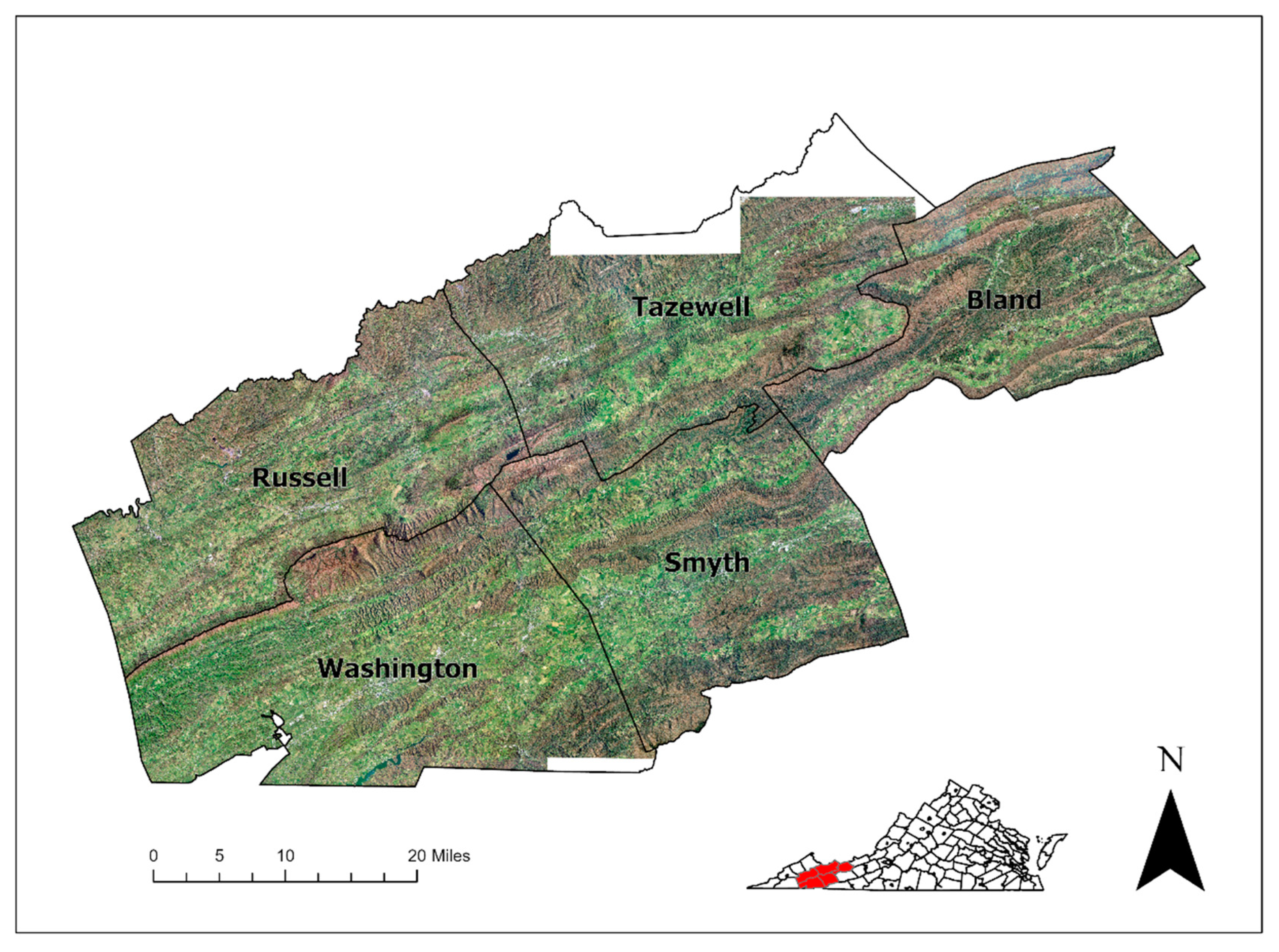
2.1. Study Area

Using a system representative of the region’s heterogeneous terrain and ecosystems, our goal was to create a de novo classification that includes seven ecologically relevant classes: shrub/sapling, pasture, human infrastructure (buildings and roads), bare ground, water, and evergreen and deciduous/mixed forest. We focused our classification in five counties in southwestern Virginia—Smyth, Tazewell, Russell, Washington, and Bland (Figure 1)—that cover >6000 km2 with cover types representative of the broader southern and central Appalachian regions. The counties are mountainous, with a mean elevation of 760 m range (403–1746 m) and ridges running primarily southwest to northeast. George Washington and Jefferson National Forests comprise ~20% of the landscape, and many mountain ridges are primarily forested. Forests are primarily oak-hickory and to a lesser extent mixed oak-pine on dryer slopes with spruce along the highest ridges [32]. Past and present coal mining activity occurs in a narrow portion of northwestern Russell and Tazewell Counties. Based on NLCD data, 64% of the region is forested and 25% is pasture/grassland; agricultural production occurs primarily in the valleys where much of the land is used for hay and livestock production. Shrub/sapling cover tends to occur along the forested edges of pasture and expand into pastures when grazing pressure is low, as well as in regenerating timber harvests.

2.2. Predictor Raster Acquisition and Processing

We acquired 1 m resolution orthoimagery collected through NAIP as a four-band (red, green, blue, and near-infrared) spectral image collected during April 2016. NAIP imagery is typically collected during the agricultural growing season such that it represents ‘leaf-on’ imagery, but only trees in the lowest elevations of this mountainous region have begun to leaf out in April. Images were collected on either April 18 or 24; though portions were removed prior to classification from the northern and southern extremes of our study area because they were collected in a different season (Figure 1). Because images across such a large region are collected on different days and times of day, there can be within-class variations in spectral properties, variable viewing geometry, and illumination [33]. Despite these challenges, NAIP imagery has been successfully used for land cover classification and feature extraction [33,34,35]. We also acquired 1 ft resolution orthophotography through the Virginia Base Mapping Program (hereafter VBMP) [31]. This is a three-band image (RGB) and was collected via flyover with a digital camera during the winter ‘leaf-off’ period of 2016 (January). Using imagery from different seasons is helpful in land cover classifications because seasonal patterns can be used to differentiate cover types [36,37]. We resampled the VBMP imagery to 1 m resolution and aligned it with NAIP imagery. For one of the focal counties (Washington), VBMP imagery was not available for a large portion of the county so we carried out all classification steps but excluded VBMP imagery. This provided a test for the necessity of including both ‘leaf-on’ and ‘leaf-off’ imagery to accurately classify shrub/sapling cover.
We performed image segmentation separately on both NAIP and VBMP imagery using the mean-shift segmentation tool in ArcGIS Pro (version 2.7). Segmentation groups nearby cells sharing similar spectral characteristics and has been shown to reduce graininess in final classifications [12]. Spectral detail, spatial detail, and minimum segment size must be set during segmentation, and we selected values for these parameters that best identified image objects (roads, houses, clumps of shrub/saplings, patches of forest, etc.) in the landscape. We consistently used a spatial detail value of 14 and minimum segment size of 8, and we selected spectral detail values of 17 or 18 for each county, based on visual inspection of resulting image segments. Segmentation produces a three-band raster where each cell in an image object has the same values for each spectral band. Because NAIP has four bands, we used green, blue, and NIR bands for segmentation because they were most distinct from each other (Figure 2).
We created two additional raster layers from the VBMP and NAIP imagery. Normalized difference vegetation index (hereafter NDVI), which characterizes vegetation “greenness”, was calculated from NAIP imagery and may help to discriminate shrub/sapling, pasture, and forest classes [38]. A texture metric was calculated using the focal statistics tool in ArcGIS Pro to describe the standard deviation of cells in a 5 × 5 m window using the red band from the ‘leaf-off’ VBMP image. In a preliminary study [39], this window size and band were shown to predict the shrub/sapling class better than others from VBMP and NAIP. Such texture metrics have been shown to effectively predict patchy, shrubby habitat [40], and visual observation of texture rasters with different window sizes suggested that the texture of shrub was captured at a 5 m scale.
We acquired 1/3 arc-second (approximately 10 m) resolution elevation data from the USGS National Elevation Dataset (hereafter NED). We resampled NED to 1 m resolution using bilinear interpolation and aligned it with NAIP imagery. Because we are working in a mountainous region, we needed to account for variation in reflectance resulting from differences in slope and aspect. We calculated the terrain layers of slope and aspect from our digital elevation model (DEM) using ArcGIS Pro.
We batch downloaded 1 m resolution Light Detection and Ranging (LIDAR) discrete point cloud data from the United States Geological Survey ftp site (rockytopftp.cr.usgs.gov, accessed 27 September 2020). LIDAR data were collected in the focal region between November 2016 and April 2017, and had high density point clouds (often 6–10+ points per square meter and never <2, and LIDAR base specifications version 2.1 [USGS, 2019b]). We downloaded compressed LAS files (.laz), and used the lidR package (Roussel et al. 2020) in R (version 4.0.2, [41]) to process files within subregions of each county and to create a 1 m resolution canopy height model raster from the LIDAR point cloud using the grid_canopy function.
These steps resulted in 13 individual raster layers (Figure 2) that we used as predictors in a pixel-based Random Forest Classification model: three bands (RGB) for the segmented VBMP; three bands (G, B, and NIR) for the segmented NAIP; the red band from the NAIP imagery; NDVI, the texture metric, elevation, slope, aspect, and a LIDAR-derived canopy height model. All rasters were exported as GeoTIFFs for random forest modeling in the R statistical software. One county (Washington) did not have usable VBMP data, so we used nine predictor rasters for that county and provided a useful test case for carrying out the same classification methodology, but with imagery from only one time of year.
The southwestern Virginia region presents some unique problems for classification. It is mountainous, which creates shadowed regions in aerial imagery that results in the same land cover classes having different spectral signatures depending on their location on the landscape. To account for this, we incorporated the aspect of the land surface, or the direction that the slope is facing, as an input to our classification scheme. We also subdivided certain land cover classes during training data creation into sun and shade subcategories (see below). To minimize the impacts of phenological differences in leaf out in our mountainous study region, and because of high computing demands for high resolution data, we carried out the land cover classification steps separately for each county and then mosaicked the resulting land cover maps together.

2.3. Training Data

We created training data using the segmented ‘leaf-on’ and ‘leaf-off’ orthoimagery described above. Specifically, we used the Training Samples Manager in ArcGIS Pro to create polygons around areas of known cover types by systematically panning across each county. Our selection of training data was informed by visual inspection of the input layers described above and on-the-ground experience conducting bird surveys in the region. We primarily used the segment picker tool in the Training Samples Manager, such that polygons corresponded to image segments, but also occasionally selected smaller areas by drawing polygons when we needed to isolate a cover type that was not identified as a segmented object (i.e., group of evergreen trees within an otherwise deciduous forest object). We adapted the NLCD2011 Training schema in ArcGIS by removing wetland and adding shadow subclasses (i.e., shadow deciduous forest, shadow impervious surface, and shadow pasture) that were later merged with non-shadow classes of the same cover type. Some patches of vegetation were difficult to differentiate from forest or shrub/sapling via visual inspection. In these cases, we consulted the LIDAR-derived canopy height model to designate training polygons as shrub/sapling when canopy height was ≤4 m and as forest when canopy height was >4 m. We pixelated the training polygons using the polygon to raster tool and then the raster to polygon tool so that polygons would line up perfectly with the predictor rasters. In total, we created 5368 training polygons that covered 1200 ha and comprised 0.096% of the focal region.

2.4. Random Forest Classification

We used a Random Forests Classification framework [42,43] to classify the different land cover types of interest. Random Forests is a powerful classification tool that tends to have a high rate of accuracy, the ability to handle large datasets, and is less computationally intensive than methods with comparable accuracy [42]. The algorithm is a bootstrapping ensemble method that operates by averaging a large number of randomly generated decision trees for a single final model with low variance and high accuracy [43].
Classification was performed using the randomForests [44] and raster [45] packages in R (version 4.0.2). We extracted mean values for each of the 13 predictor rasters in the training polygons described above, and used these values as inputs into the random forest algorithm. Because the random forest algorithm uses bootstrapped samples for generating each decision tree, we can assess preliminary model performance based on the training dataset. We assessed which prediction rasters are most important in predicting each cover type using the variable importance scores from the Random Forest output. We created a classification raster based on the random forest model using the predict function in the R raster package [45]. We then informally inspected the land cover classification by comparing it to the NAIP imagery to preliminarily gauge its performance. If cover classes were consistently misclassified (e.g., tree shadows in pasture being classified as water), we created more training data (e.g., created a new class called ‘shadow pasture’ to be later merged with pasture) in the problem areas and repeated the random forest classification. Once we were satisfied with the classification based on informal inspection, we carried out two post-processing steps prior to a formal accuracy assessment. First, we removed noise from the classification raster using the majority filter function with four neighbors in ArcGIS Pro. Second, we combined the shadow classes with the major cover type (e.g., merged shadow pasture with pasture) by reclassifying the raster. The resulting map had seven land cover classes: shrub/sapling (woody deciduous vegetation between 0.5–4 m tall), pasture (includes hayfields, grassland, and cultivated fields), human infrastructure (roads, buildings, etc.), bare ground (gravel roads and patches of bare soil), water (rivers, streams, lakes, and ponds), mixed/deciduous forest (woody deciduous vegetation >4 m), and evergreen forest (woody evergreen vegetation).

2.5. Accuracy Assessment

To assess accuracy of the land cover classification, we followed recent recommendations in Stehman and Foody [46] for image interpretation using an independent sample of validation points from those used in training the classification model. We generated a stratified random sample of 100 validation points per cover type in each county, though 100 points were not always possible for rare cover types (i.e., water). We created a 3 m buffer around each validation point and extracted the majority land cover type and the number of cover types in each buffer from the final classified raster. We deleted validation points with ≥4 cover types within the buffer (19.7% of validation points) because of the difficulty in discerning the reference cover type in such complex settings (i.e., reference class ambiguity, [46]). This is especially problematic for high resolution classifications. Ideally, validation is carried out with imagery that is different and of finer resolution than the imagery used to develop the classified map; however, this is not always possible when using high-resolution imagery for classification [46]. The result is that accuracy may be over-estimated, particularly in areas with significant cover type heterogeneity. The majority value within each buffer serves as the predicted value for accuracy assessment. A single observer (LPB) that was naïve to the predicted values determined the actual/reference land cover based on visual inspection (human interpretation) of the NAIP and VBMP imagery within the 3 m buffers. The observer would indicate the primary cover type within the buffer as well as the secondary cover type when two cover types occurred in similar amounts within the buffer (i.e., the point fell along the edge of a road and a pasture). We deleted any points where significant changes occurred between the NAIP and VBMP images (e.g., a timber harvest between January and April 2016), but this only occurred in a small number (<5%) of points. Finally, we compared the observer’s primary or secondary cover type designation to the reference value extracted from the final classified raster to assess accuracy [47]. Specifically, we used the caret package [48] in R to calculate a confusion matrix and accuracy metrics.

2.6. Comparison with Publicly Available Land Cover Data

To compare our custom land cover map to the widely used NLCD, we calculated composition landscape metrics for our custom classification at fine (1 m) and coarse (resampled to 30 m) resolutions using the landscapemetrics package in R [49] and compared these to metrics calculated from NLCD (30 m). Specifically, we calculated the percent cover for pasture/grassland, shrub/sapling, and deciduous/mixed forest within a 500 m radius around randomly placed points within pre-defined areas of early successional habitat—open areas with a mix of pasture, shrub and sapling cover but in a forested landscape. We placed points in these areas because a random sample of points across the entire region would not have effectively captured the less common shrub/sapling cover which is the focus of this study. For NLCD, we combined deciduous and mixed forest to create one forest class, and combined pasture and herbaceous cover to create one pasture/grassland class. NLCD has recently added a transitional forest classes (shrub-forest) that is based on time since forest clearing and known successional rates for different regions. We combined the shrub/scrub with this shrub-forest class to create one shrub class. We used linear regression analysis to assess the correlation between NLCD and both fine- and coarse-resolution custom land cover.
Land cover output and canopy height models for each county, as well as the R scripts used for this research, are available on Dryad Data Depository (https://doi.org/10.5061/dryad.jsxksn0b1, accessed on 6 January 2022). Training data shapefiles and accuracy assessment points are available upon request from the authors.

3. Results

3.1. Classification Accuracy

The overall accuracy of the final land cover classification across the >6000 km2 focal region was 89.1%. Producer accuracies (i.e., how often on the ground features are correctly shown in the classified map) for each individual class were between 81% and 99% and user accuracies (how often the map classification actually represents what is on the ground) for each class were between 82% and 95% (Table 1). Though classification accuracy was generally high, the most common misclassifications included confusion between deciduous/mixed and evergreen forest, between bare ground and human development, and between bare ground and pasture (Table 1). The shrub/sapling class, of primary importance in this study, had high classification accuracy (≥90%).
The confusion matrices for land cover accuracy for individual counties are provided in the Supplementary Information (Table S1) and show that when leaf off imagery (VBMP) is not included in the classification (i.e., Washington County), accuracy was very similar for all cover types.

3.2. Predictor Importance

The random forest algorithm ranks classification predictor variables based on importance for discriminating each land cover class (Table 2). The LIDAR-derived canopy height model ranked as the most important predictor for all vegetative cover types and within the top three predictors for water and developed land covers. NDVI was the second-most important predictor, and ranked highly for nearly all cover types. Bands from ‘leaf-on’ imagery (NAIP) tended to rank higher than bands from ‘leaf-off’ imagery (VBMP); however, the red band for VBMP was in the top three most important predictor variables for shrub/sapling and evergreen forest (Table 2). Of the three terrain metrics, elevation consistently ranked higher than slope and aspect, but generally were less informative than spectral variables and the canopy height model. For the shrub/sapling cover class, the canopy height model, NDVI, and the red band of the VBMP leaf-off imagery were the three most important variables. Figure 3 shows side-by-side comparisons of NAIP imagery, the canopy height model, and our custom classification for two example landscapes in our study area.

3.3. Comparison with Publicly Available Land Cover Data

Compared with NLCD, our 1 m land cover classification more accurately represents fine-scale features such as ponds and patches of shrubs/saplings, but also captures patches of forest and pasture/grassland that are obscured by the coarser-resolution NLCD (Figure 4). Across the extent of our five-county focal region, our land cover classification has some similarities with the publicly available NLCD and fine-resolution VLCD; however, there are some important differences (Table 3). Our custom classification under-represents developed land cover compared with NLCD and over-represents barren land cover compared with both NLCD and VLCD, but the sum of these often-similar classes is similar among the three classifications (2.2–6.4%). Our custom classification identifies more evergreen forest and less deciduous forest than NLCD; some of this may be due to misclassifications between deciduous/mixed and evergreen forest in our custom classification. However, when we sum deciduous/mixed and evergreen forest cover, NLCD and VLCD still show ~3–7% more total forest cover across the focal landscape than our custom classification (Table 3). At least some of this discrepancy is likely due to the omission of shrub/sapling cover from the publicly available land cover datasets that is captured in our custom classification.
Comparing land cover maps across entire counties can uncover general trends, but assessing differences in focal areas can be valuable when a specific and less common cover type is of interest. We compared composition landscape metrics calculated from NLCD and our custom classification within 500 m around random points in early successional habitats that have a mix of pasture, forest and shrub/sapling cover. We found that pasture cover from NLCD was highly correlated with pasture cover in our fine resolution custom classification (r = 0.858; Figure 5a) and when our custom classification was resampled to 30 m resolution (r = 0.870; Figure 5b). The same was true for forest cover from NLCD and forest cover in our fine resolution custom classification (r = 0.825; Figure 5a) and when our custom classification is resampled to 30 m resolution (r = 0.823; Figure 5b). Despite these strong correlations, compared with our custom classification, NLCD underrepresented pasture/grassland cover by ~10% in areas with low pasture cover and over-represents forest cover by ~10–25%, especially in predominantly forested areas. These differences exist even when we resampled our custom classification to be the same 30 m resolution as NLCD (Figure 5b). Further, there is no correlation between NLCD and our custom classification with regard to shrub/sapling cover (r < 0.1, Figure 5c,d). Our custom classification has values of 0 to 35% shrub/sapling cover while NLCD has most values < 5% and a few as high as 11%, and many areas in our custom classification with the highest values for shrub cover (>20%) have 0% shrub in NLCD.

4. Discussion

The land cover classification framework presented here exceeded initial goals of at least 80% accuracy for each land cover class and accurately represents shrub/sapling cover at a fine resolution across a large focal region (>6000 km2). This is significant because shrub/sapling is an ecologically important cover type that is nearly absent in publicly available NLCD data for the eastern United States, and recent efforts to classify shrub cover have proved challenging [50,51]. Shrubs make up 21.7% of the NLCD land cover in the conterminous United States, but this cover type is primarily concentrated in the arid western states [52] where shrubs are spectrally different from other cover types (i.e., sage (Artemisia spp.) compared to trees and grasses). The framework we present here relies on freely available data through the United States Department of Agriculture (NAIP) and the United States Geological Survey (high-resolution LIDAR; [53]). Because our custom classification relies on LIDAR-derived canopy height models in addition to spectral properties of cover types from satellite imagery, we were able to identify shrubs that would otherwise appear spectrally similar to forests and be classified as such. Our findings also show that accurate representation of shrub/sapling cover is not completely dependent on the grain of the classified map; our classification resampled to 30 m resolution still represented shrub cover better than NLCD.
A LIDAR-derived canopy height model was the most important predictor (i.e., it had the highest variable importance value in our random forest model) for all vegetation cover types and was the second and third most important predictor for water and developed cover types, respectively. This makes sense considering the fact that these different cover types are defined in part by their relative heights; trees are taller than shrubs/saplings which are taller than pasture/grassland, and previous studies have shown LIDAR to improve the accuracy of classifying of shrubs [50]. Our study also showed that LIDAR-derived canopy heights overshadowed any benefits of using imagery from different seasons to discriminate vegetation cover types. Specifically, the limited availability of leaf-off imagery in one of our focal counties provided a test for the necessity of including both ‘leaf-on’ and ‘leaf-off’ imagery to accurately classify shrub cover. Both image types were expected to provide important spectral information to discriminate trees from shrub/saplings through seasonal differences in reflectance. However, LIDAR data proved able to discriminate between these and other cover types without the two different seasons of imagery. This finding is significant because acquisition of high-resolution data across large focal regions involves significant time and effort. We recommend that future efforts rely primarily on freely available leaf on imagery (i.e., NAIP) and high-resolution data on vegetation structure (i.e., LIDAR) to accurately classify shrub/sapling cover alongside other major cover types.
Despite the importance of the LIDAR-derived canopy height model, spectral information was still important in helping to discriminate different cover types, especially those with LIDAR heights < 0.5 m. The value of NDVI in discriminating vegetation cover types from non-vegetative cover types and in discriminating different vegetation cover types over space (biomass and health) and time (phenology) is well established [54,55,56,57,58,59]. This study further demonstrates the value of NDVI as it was the first or second most important predictor for all cover types except barren areas. Other spectral predictors (NAIP Red, Blue, Green, and VBMP Blue) were among the top three predictors that helped to discriminate between cover types with low LIDAR heights (<0.5 m). For example, water, pasture/grassland, bare soil, and roads are all at the ground level but show different spectral properties that are even discernable in imagery with low spectral resolution, such as the freely available NAIP imagery [7]. Indeed, the use of LIDAR-derived height data helps to mitigate the challenge of working with low spectral resolution NAIP imagery while still taking advantage of the high spatial resolution spectral information and wide availability across the conterminous US [60].
A non-trivial challenge of classifying a shrub/sapling cover type is their ephemeral nature; saplings and shrubs often rapidly grow into closed-canopy forests. Mine lands, high intensity grazed lands, and some very high elevation areas are exceptions to this as their heavily compacted soils and/or harsh climate slow the rate of succession and result in the persistence of shrub/saplings for many decades. Disturbance-prone systems such as flooded riparian areas are another dynamic system that has been a focus of classification studies [61,62]. Climate change is impacting disturbance regimes globally [63] and high temporal resolution of remotely sensed imagery is needed for understanding how biodiversity and landscape processes will be affected [64,65]. Therefore, collection of remotely sensed imagery and canopy height data with high temporal resolution is necessary to facilitate frequent updates to publicly available regional and national land cover classification maps. Landsat and NAIP imagery are collected with a high temporal resolution (16 days and 3–5 years, respectively) that is compatible with modeling disturbance-prone systems with shrub/sapling cover; however, LIDAR data have only recently become available for many parts of the conterminous US and it is uncertain how often these data will be updated. For small focal areas, LIDAR data collected via unmanned aerial vehicles is a good option [66,67,68]; however, natural resource management efforts typically require large extents that make such collection methods less viable. The multitude of uses for LIDAR data to model dynamic systems at large spatial extents—from detecting and modeling flooding, landslides, shrub expansion, and coastal erosion, to assessments of forest canopy structure, forest carbon stocks, and wildlife habitats—make it a priority to collect with high temporal resolution. Recently, a global canopy height map was developed by combining Landsat imagery and LIDAR data from Global Ecosystem Dynamics Investigation (GEDI) and allows for production of annual forest height maps [18], though the spatial resolution is too coarse (30 m) to capture small features such as individual shrubs and saplings.

4.1. Comparison with Publicly Available Land Cover Data

It is well established that coarse grained data do not accurately represent the complexity of small features on the landscape [69,70,71], yet our study demonstrates that grain is not the only factor explaining the poor representation of shrub/sapling cover in NLCD. Even after resampling our land cover classification to 30 m resolution, shrub/saplings were still represented significantly more than in publicly available maps with fine and coarse resolution (VLCD and NLCD, respectively), and it more accurately represents the vegetation cover types present on the landscape. If we had observed a significant loss of shrub/sapling cover from our resampled classification, that would suggest that shrubs are typically distributed in isolated and small clumps. In reality, many species of shrub/saplings in our system (Rubus spp., Cretaegus spp., and Robinia pseudoacacia) tend to exist in large clumps in abandoned and lightly grazed pastures; likewise, regenerating saplings following timber harvests also grow in large clumps that would be captured with coarse resolution data. However, we did observe a reduction in shrub cover by ~5% when we resampled to a coarser resolution map indicating that some shrubs and saplings do occur in small, isolated clumps and will be lost from coarse grained maps.
Although grain is not the primary factor explaining the poor representation of shrub/saplings in NLCD, the absence of information on vegetation height likely is. Publicly available land cover maps such as NLCD rely on time series Landsat multi-spectral imagery and do not incorporate canopy height information into their classification methodology [72]. Time series Landsat data should allow for the detection of forest disturbances that occur between consecutive images and, coupled with expert knowledge of forest succession in different regions, can infer the presence of transitional forest classes [72]. However, misclassification errors between shrub/sapling and herbaceous and between shrub/sapling and forest are common in NLCD [72], likely due to the spectral similarity of these cover types. Our study corroborates this and shows that the shrub-forest transition class does not accurately represent shrub/sapling cover in our focal region in the Appalachian Mountains. Increased availability of global canopy height data [18], albeit at coarser resolution (30 m) than used here, will hopefully result in a more accurate representation of shrub/saplings in future releases of NLCD data and similar maps in other countries. Even coarse resolution canopy height data will capture larger patches of shrubs and regenerating timber harvests and be a significant improvement over the current NLCD. The loss of information about small patches of shrub/sapling cover due to coarse resolution vegetation structure data may be acceptable depending on the goals of the study. For example, if the amount of shrub/sapling cover at large spatial extents (entire states or multi-state regions) is of interest, then working with 30 m resolution data may be necessary to decrease computer processing time and power required. Range-wide distribution models for shrub-dependent species or continental scale models of forest impacts on carbon budgets are examples of such large-scale applications where coarse resolution data would be preferred. If, however, the spatial configuration/arrangement of shrub/saplings, even small clumps, is of interest, then maintaining fine resolution data (1 m) will be necessary and the spatial extent of analyses will have to be limited to smaller areas (e.g., a county or locality).

4.2. Limitations

This study used LIDAR to create a canopy height model that captures the top of canopy height only and does not include information about the presence or structure of vegetation in the forest understory. Understory vegetation, including shrubs, saplings, and herbaceous cover, is important ecologically as it contributes to wildlife habitat [73], forest microclimate [74], and carbon stocks [75]. However, the high variation in sampling density of LIDAR point clouds make it difficult to accurately predict understory vegetation structure, though efforts to make this possible are ongoing [76]. Future efforts to represent shrub/sapling cover in land cover classification maps should consider the inclusion of understory woody vegetation as well; forests with a woody understory would be a different class than forests without a woody understory.
The accuracy of our land cover classification may be over-estimated, especially in areas with a complex mosaic of cover types. One of the challenges of working with high resolution (1 m) data is the difficulty in assessing the accuracy of every pixel. As a result, regions of several pixels (in our case 3 m buffers) are used for validation and there will inevitably be variation in cover types within some of these regions leading to reference class ambiguity [46]. We used recommended methods for dealing with this ambiguity; however, we deleted the most heterogeneous validation points (≥4 cover types within 3 m buffer) because we were not confident in our ability to assign a reference class based on visual interpretation of imagery in these complex areas. Because these accounted for ~20% of our validation points, we expect that the true accuracy of our classification is not as high as reported. That said, to our knowledge, this is the first effort to classify shrub/sapling cover across a large geographic area in the mountainous and mesic eastern United States, and our classification is a significant improvement over NLCD and other land cover classifications in its representation of shrub/sapling cover.
Due to limitations in funding, we were not able to assess the accuracy of our classified map through ground truthing, yet we are confident in our findings for two reasons. First, we conducted bird surveys in early successional habitats throughout the focal region in 2018 and 2019 and are familiar with the distribution and growth form of shrubs and saplings in this system. The motivation for this study resulted from our desire to model bird-habitat relationships for shrub-dependent species, and the lack of suitable land cover data with an accurate representation of shrub/saplings to meet our objectives. Second, we were confident in our ability to visually interpret actual land cover during our accuracy assessment from the high resolution NAIP and VBMP imagery, and followed the recommendations of Stehman and Foody [46] to carry out a rigorous accuracy assessment. By removing complex areas (i.e., those with ≥4 cover types within our 3 m buffer) from our accuracy assessment we may be ignoring some mis-classifications of very small objects (<3 m), but accuracy assessment is not possible on a per-pixel basis with high-resolution (1 m) classifications. Had we used OBIA to classify land cover rather than a pixel-based classification of segmented imagery, there would likely be fewer complex accuracy points removed from our assessment. Proposed future improvements to the SegOptim package [77] may make this possible for studies such as ours with large extents and high resolution.

5. Conclusions

In this study, we present a fine-resolution land cover classification framework that utilizes publicly available spatial data to accurately identify shrubs in a heavily forested, mountainous region of the eastern United States where shrub/sapling cover is typically under-represented in publicly available land cover datasets. A LIDAR-derived canopy height model enabled discrimination of spectrally similar shrub/saplings and trees and was the most important predictor of all vegetative cover types. Spatial resolution was not the only factor explaining the poor representation of shrub cover in NLCD; when we resampled our land cover classification to 30 m resolution, shrubs were still represented significantly more than in NLCD. These findings point to the need for fine spatial and temporal resolution canopy height data to accurately identify shrub/sapling cover due to their patchy distribution, ephemeral nature, and ecological importance. We demonstrate a reproducible framework for creating accurate custom land cover classifications that can be used to improve our understanding of ephemeral and complex systems such as early successional habitats with a mix of pasture/grassland and shrub/sapling cover types.

Supplementary Materials

The following supporting information can be downloaded at: https://www.mdpi.com/article/10.3390/rs14061364/s1, Table S1: Confusion matrices for each of the five counties.

Author Contributions

Conceptualization, E.S. and L.B.; Methodology, E.S., L.B. and B.L.; Validation, L.B.; Formal Analysis, L.B. and B.L.; Data Curation, E.S.; Writing—Original Draft Preparation, E.S., L.B. and B.L.; Writing—Review & Editing, L.B. and B.L.; Visualization, L.B. and B.L.; Supervision, L.B.; Project Administration, L.B.; Funding Acquisition, L.B. All authors have read and agreed to the published version of the manuscript.

Funding

This research was carried out with funds provided by the Virginia Department of Wildlife Resources (EP2815408) through a Federal Aid in Wildlife Restoration grant from the U.S. Fish and Wildlife Service.

Data Availability Statement

Land cover output and canopy height models for each county, as well as R scripts used for this research are available on Dryad Data Depository (https://doi.org/10.5061/dryad.jsxksn0b1, accessed on 6 January 2022). Training data shapefiles and accuracy assessment points are available upon request from the authors.

Acknowledgments

We are grateful to V. Thomas for guidance with downloading and processing LIDAR data and to S. Harding, S. Rogers, A. Balmer, N. Novak, and C. Gough for thoughtful input on an earlier version of the manuscript.

Conflicts of Interest

The authors declare no conflict of interest.

References

  1. With, K. Essentials of Landscape Ecology; Oxford University Press: Oxford, UK, 2019; ISBN 978-0198838395. [Google Scholar]
  2. Homer, C.; Dewitz, J.; Yang, L.; Jin, S.; Danielson, P.; Xian, G.; Coulston, J.; Herold, N.; Wickham, J.; Megown, K. Completion of the 2011 national land cover database for the conterminous United States—Representing a decade of land cover change information. Photogramm. Eng. Remote Sens. 2015, 81, 345–354. [Google Scholar] [CrossRef]
  3. Grêt-Regamey, A.; Weibel, B.; Bagstad, K.J.; Ferrari, M.; Geneletti, D.; Klug, H.; Schirpke, U.; Tappeiner, U. On the effects of scale for ecosystem services mapping. PLoS ONE 2014, 9, e112601. [Google Scholar] [CrossRef] [PubMed]
  4. Rioux, J.F.; Cimon-Morin, J.; Pellerin, S.; Alard, D.; Poulin, M. How land cover spatial resolution affects mapping of urban ecosystem service flows. Front. Environ. Sci. 2019, 7, 93. [Google Scholar] [CrossRef]
  5. Xie, Y.; Sha, Z.; Yu, M. Remote sensing imagery in vegetation mapping: A review. J. Plant Ecol. 2008, 1, 9–23. [Google Scholar] [CrossRef]
  6. Moskal, L.M.; Styers, D.M.; Halabisky, M. Monitoring urban tree cover using object-based image analysis and public domain remotely sensed data. Remote Sens. 2011, 3, 2243–2262. [Google Scholar] [CrossRef] [Green Version]
  7. Hayes, M.M.; Miller, S.N.; Murphy, M.A. High-resolution landcover classification using random forest. Remote Sens. Lett. 2014, 5, 112–121. [Google Scholar] [CrossRef]
  8. Gonçalves, J.; Henriques, R.; Alves, P.; Sousa-Silva, R.; Monteiro, A.T.; Lomba, Â.; Marcos, B.; Honrado, J. Evaluating an unmanned aerial vehicle-based approach for assessing habitat extent and condition in fine-scale early successional mountain mosaics. Appl. Veg. Sci. 2016, 19, 132–146. [Google Scholar] [CrossRef] [Green Version]
  9. Davies, K.W.; Petersen, S.L.; Johnson, D.D.; Davis, D.B.; Madsen, M.D.; Zvirzdin, D.L.; Bates, J.D. Estimating juniper cover from national agriculture imagery program (NAIP) imagery and evaluating relationships between potential cover and environmental variables. Rangel. Ecol. Manag. 2010, 63, 630–637. [Google Scholar] [CrossRef]
  10. Maxwell, A.E.; Strager, M.P.; Warner, T.A.; Zégre, N.P.; Yuill, C.B. Comparison of NAIP orthophotography and rapideye satellite imagery for mapping of mining and mine reclamation. GIScience Remote Sens. 2014, 51, 301–320. [Google Scholar] [CrossRef]
  11. Hurskainen, P.; Adhikari, H.; Siljander, M.; Pellikka, P.K.E.; Hemp, A. Auxiliary datasets improve accuracy of object-based land use/land cover classification in heterogeneous savanna landscapes. Remote Sens. Environ. 2019, 233, 111354. [Google Scholar] [CrossRef]
  12. Laliberte, A.S.; Rango, A. Texture and scale in object-based analysis of subdecimeter resolution unmanned aerial vehicle (UAV) imagery. IEEE Trans. Geosci. Remote Sens. 2009, 47, 761–770. [Google Scholar] [CrossRef] [Green Version]
  13. Ma, L.; Li, M.; Ma, X.; Cheng, L.; Du, P.; Liu, Y. A review of supervised object-based land-cover image classification. ISPRS J. Photogramm. Remote Sens. 2017, 130, 277–293. [Google Scholar] [CrossRef]
  14. Aguirre-Gutiérrez, J.; Seijmonsbergen, A.C.; Duivenvoorden, J.F. Optimizing land cover classification accuracy for change detection, a combined pixel-based and object-based approach in a mountainous area in Mexico. Appl. Geogr. 2012, 34, 29–37. [Google Scholar] [CrossRef] [Green Version]
  15. Salehi, B.; Zhang, Y.; Zhong, M. A combined object- and pixel-based Image Analysis Framework for Urban Land Cover classifiation of VHR Imagery. Photogramm. Eng. Remote Sens. 2013, 79, 999–1014. [Google Scholar] [CrossRef]
  16. Martinuzzi, S.; Vierling, L.A.; Gould, W.A.; Falkowski, M.J.; Evans, J.S.; Hudak, A.T.; Vierling, K.T. Mapping snags and understory shrubs for a LiDAR-based assessment of wildlife habitat suitability. Remote Sens. Environ. 2009, 113, 2533–2546. [Google Scholar] [CrossRef] [Green Version]
  17. Estornell, J.; Ruiz, L.A.; Velázquez-Martí, B.; Hermosilla, T. Estimation of biomass and volume of shrub vegetation using LiDAR and spectral data in a Mediterranean environment. Biomass Bioenergy 2012, 46, 710–721. [Google Scholar] [CrossRef] [Green Version]
  18. Potapov, P.; Li, X.; Hernandez-Serna, A.; Tyukavina, A.; Hansen, M.C.; Kommareddy, A.; Pickens, A.; Turubanova, S.; Tang, H.; Silva, C.E.; et al. Mapping global forest canopy height through integration of GEDI and Landsat data. Remote Sens. Environ. 2021, 253, 112165. [Google Scholar] [CrossRef]
  19. U.S. Geological Survey. The National Map—New Data Delivery Homepage, Advanced Viewer, Lidar Visualization: US. Geological Survey Fact Sheet 2019–3032; U.S. Geological Survey: Reston, VA, USA, 2019; Volume 2.
  20. Greaves, H.E.; Vierling, L.A.; Eitel, J.U.H.; Boelman, N.T.; Magney, T.S.; Prager, C.M.; Griffin, K.L. High-resolution mapping of aboveground shrub biomass in Arctic tundra using airborne lidar and imagery. Remote Sens. Environ. 2016, 184, 361–373. [Google Scholar] [CrossRef]
  21. Cleve, C.; Kelly, M.; Kearns, F.R.; Moritz, M. Classification of the wildland-urban interface: A comparison of pixel- and object-based classifications using high-resolution aerial photography. Comput. Environ. Urban Syst. 2008, 32, 317–326. [Google Scholar] [CrossRef]
  22. Askins, R.A. Sustaining biological diversity in early successional communities: The challange of managing unpopular habitats. Wildl. Soc. Bull. 2001, 29, 407–412. [Google Scholar] [CrossRef]
  23. King, D.I.; Schlossberg, S. Synthesis of the conservation value of the early-successional stage in forests of eastern North America. For. Ecol. Manage. 2014, 324, 186–195. [Google Scholar] [CrossRef]
  24. Besnard, S.; Carvalhais, N.; Arain, M.A.; Black, A.; De Bruin, S.; Buchmann, N.; Cescatti, A.; Chen, J.; Clevers, J.G.P.W.; Desai, A.R.; et al. Quantifying the effect of forest age in annual net forest carbon balance. Environ. Res. Lett. 2018, 13, 124018. [Google Scholar] [CrossRef] [Green Version]
  25. Ciais, P.; Dolman, A.J.; Bombelli, A.; Duren, R.; Peregon, A.; Rayner, P.J.; Miller, C.; Gobron, N.; Kinderman, G.; Marland, G.; et al. Current systematic carbon-cycle observations and the need for implementing a policy-relevant carbon observing system. Biogeosciences 2014, 11, 3547–3602. [Google Scholar] [CrossRef] [Green Version]
  26. Singh, K.K.; Vogler, J.B.; Shoemaker, D.A.; Meentemeyer, R.K. LiDAR-Landsat data fusion for large-area assessment of urban land cover: Balancing spatial resolution, data volume and mapping accuracy. ISPRS J. Photogramm. Remote Sens. 2012, 74, 110–121. [Google Scholar] [CrossRef]
  27. Hartfield, K.A.; Landau, K.I.; van Leeuwen, W.J.D. Fusion of high resolution aerial multispectral and lidar data: Land cover in the context of urban mosquito habitat. Remote Sens. 2011, 3, 2364–2383. [Google Scholar] [CrossRef] [Green Version]
  28. Ucar, Z.; Bettinger, P.; Merry, K.; Akbulut, R.; Siry, J. Estimation of urban woody vegetation cover using multispectral imagery and LiDAR. Urban For. Urban Green. 2018, 29, 248–260. [Google Scholar] [CrossRef]
  29. Buehler, D.A.; Roth, A.M.; Vallender, R.; Will, T.C.; Confer, J.L.; Canterbury, R.A.; Swarthout, S.B.; Rosenberg, K.V.; Bulluck, L.P. Status and conservation priorities of Golden-winged Warbler (Vermivora chrysoptera) in North America. Auk 2007, 124, 1439–1445. [Google Scholar] [CrossRef]
  30. Albrecht-Mallinger, D.J.; Bulluck, L.P. Limited evidence for conspecific attraction in a low-density population of a declining songbird, the Golden-winged Warbler (Vermivora chrysoptera). Condor 2016, 118, 451–462. [Google Scholar] [CrossRef]
  31. WorldView Solutions, Inc. Technical Plan of Operations: Virginia Statewide Land Cover Data Development; WorldView Solutions: Richmond, VA, USA, 2016. [Google Scholar]
  32. Rose, A.K. Virginia’s forests, 2001. In Resource Bulletin SRS-120; US Department of Agriculture Forest Service, Southern Research Station: Asheville, NC, USA, 2007; 140p. [Google Scholar] [CrossRef]
  33. Maxwell, A.E.; Strager, M.P.; Warner, T.A.; Ramezan, C.A.; Morgan, A.N.; Pauley, C.E. Large-area, high spatial resolution land cover mapping using random forests, GEOBIA, and NAIP orthophotography: Findings and recommendations. Remote Sens. 2019, 11, 1409. [Google Scholar] [CrossRef] [Green Version]
  34. Li, X.; Shao, G. Object-based land-cover mapping with high resolution aerial photography at a county scale in midwestern USA. Remote Sens. 2014, 6, 11372–11390. [Google Scholar] [CrossRef] [Green Version]
  35. Ramezan, C.A.; Warner, T.A.; Maxwell, A.E. Evaluation of sampling and cross-validation tuning strategies for regional-scale machine learning classification. Remote Sens. 2019, 11, 185. [Google Scholar] [CrossRef] [Green Version]
  36. Li, N.; Lu, D.; Wu, M.; Zhang, Y.; Lu, L. Coastal wetland classification with multiseasonal high-spatial resolution satellite imagery. Int. J. Remote Sens. 2018, 39, 8963–8983. [Google Scholar] [CrossRef]
  37. Xie, Z.; Chen, Y.; Lu, D.; Li, G.; Chen, E. Classification of land cover, forest, and tree species classes with Ziyuan-3 multispectral and stereo data. Remote Sens. 2019, 11, 164. [Google Scholar] [CrossRef] [Green Version]
  38. Defries, R.S.; Townshend, J.R. Ndvi-Derived Land Cover Classifications At a Global Scale. Int. J. Remote Sens. 1994, 15, 3567–3586. [Google Scholar] [CrossRef]
  39. Schold, E.K. Using a Custom Landscape Classification to Understand the Factors Driving Site Occupancy by a Rapidly Declining Migratory Songbird. Master’s Thesis, Virginia Commonwealth University, Richmond, VA, USA, 2018. [Google Scholar]
  40. Timm, B.C.; McGarigal, K. Fine-scale remotely-sensed cover mapping of coastal dune and salt marsh ecosystems at Cape Cod National Seashore using Random Forests. Remote Sens. Environ. 2012, 127, 106–117. [Google Scholar] [CrossRef]
  41. R Core Team. R: A Language and Environment for Statistical Computing; R Foundation for Statistical Computing: Vienna, Austria, 2020; Available online: https://www.R-project.org/ (accessed on 6 January 2022).
  42. Gislason, P.O.; Benediktsson, J.A.; Sveinsson, J.R. Random forests for land cover classification. Pattern Recognit. Lett. 2006, 27, 294–300. [Google Scholar] [CrossRef]
  43. Breiman, L. Random forests. Random For. 2019, 45, 5–32. [Google Scholar] [CrossRef]
  44. Liaw, A.; Wiener, M. Classification and Regression by randomForest. R News 2002, 2, 18–22. [Google Scholar]
  45. Hijmans, R.J.; van Etten, J. Raster: Geographic Analysis and Modeling with Raster Data. R Packag. Version 2.7-15. 2018. Available online: http://CRAN.R-project.org/package=raster (accessed on 6 January 2022).
  46. Stehman, S.V.; Foody, G.M. Key issues in rigorous accuracy assessment of land cover products. Remote Sens. Environ. 2019, 231, 111199. [Google Scholar] [CrossRef]
  47. Olofsson, P.; Foody, G.M.; Herold, M.; Stehman, S.V.; Woodcock, C.E.; Wulder, M.A. Good practices for estimating area and assessing accuracy of land change. Remote Sens. Environ. 2014, 148, 42–57. [Google Scholar] [CrossRef]
  48. Kuhn, M. Building predictive models in R using the caret package. J. Stat. Softw. 2008, 28, 1–26. [Google Scholar] [CrossRef] [Green Version]
  49. Hesselbarth, M.H.K.; Sciaini, M.; With, K.A.; Wiegand, K.; Nowosad, J. landscapemetrics: An open-source R tool to calculate landscape metrics. Ecography 2019, 42, 1648–1657. [Google Scholar] [CrossRef] [Green Version]
  50. Koetz, B.; Morsdorf, F.; van der Linden, S.; Curt, T.; Allgöwer, B. Multi-source land cover classification for forest fire management based on imaging spectrometry and LiDAR data. For. Ecol. Manag. 2008, 256, 263–271. [Google Scholar] [CrossRef]
  51. Ayhan, B.; Kwan, C. Tree, shrub, and grass classification using only RGB images. Remote Sens. 2020, 12, 1333. [Google Scholar] [CrossRef] [Green Version]
  52. Dewitz, J. National Land Cover Database (NLCD) 2016 Products (version 2.0, July 2020); Data Release; U.S. Geological Survey: Seattle, WA, USA, 2019. [CrossRef]
  53. Thatcher, C.A.; Lukas, V.; Stoker, J.M. The 3D Elevation Program and Energy for the Nation; Fact Sheet; United States Geological Survey: Seattle, WA, USA, 2020. [CrossRef]
  54. Loveland, T.R.; Merchant, J.W.; Ohlen, D.O.; Brown, J.F. Development of a land-cover characteristics database for the conterminous US. Photogramm. Eng. Remote Sens. 1991, 57, 1453–1463. [Google Scholar]
  55. Hunt, E.R. Relationship between woody biomass and PAR conversion efficiency for estimating net primary production from NDVI. Int. J. Remote Sens. 1994, 15, 1725–1730. [Google Scholar]
  56. Coops, N.C.; Johnson, M.; Wulder, M.A.; White, J.C. Assessment of QuickBird high spatial resolution imagery to detect red attack damage due to mountain pine beetle infestation. Remote Sens. Environ. 2006, 103, 67–80. [Google Scholar] [CrossRef]
  57. Verbesselt, J.; Hyndman, R.; Newnham, G.; Culvenor, D. Detecting trend and seasonal changes in satellite image time series. Remote Sens. Environ. 2010, 114, 106–115. [Google Scholar] [CrossRef]
  58. Peña-Barragán, J.M.; Ngugi, M.K.; Plant, R.E.; Six, J. Object-based crop identification using multiple vegetation indices, textural features and crop phenology. Remote Sens. Environ. 2011, 115, 1301–1316. [Google Scholar] [CrossRef]
  59. Soubry, I.; Doan, T.; Chu, T.; Guo, X. A systematic review on the integration of remote sensing and gis to forest and grassland ecosystem health attributes, indicators, and measures. Remote Sens. 2021, 13, 3262. [Google Scholar] [CrossRef]
  60. Maxwell, A.E.; Warner, T.A.; Vanderbilt, B.C.; Ramezan, C.A. Land cover classification and feature extraction from National Agriculture Imagery Program (NAIP) Orthoimagery: A review. Photogramm. Eng. Remote Sens. 2017, 83, 737–747. [Google Scholar] [CrossRef]
  61. Van Iersel, W.; Straatsma, M.; Middelkoop, H.; Addink, E. Multitemporal classification of river floodplain vegetation using time series of UAV images. Remote Sens. 2018, 10, 1144. [Google Scholar] [CrossRef] [Green Version]
  62. Morgan, B.E.; Chipman, J.W.; Bolger, D.T.; Dietrich, J.T. Spatiotemporal analysis of vegetation cover change in a large ephemeral river: Multi-sensor fusion of unmanned aerial vehicle (uav) and landsat imagery. Remote Sens. 2021, 13, 51. [Google Scholar] [CrossRef]
  63. Newman, E.A. Disturbance Ecology in the Anthropocene. Front. Ecol. Evol. 2019, 7, 147. [Google Scholar] [CrossRef] [Green Version]
  64. Kennedy, R.E.; Andréfouët, S.; Cohen, W.B.; Gómez, C.; Griffiths, P.; Hais, M.; Healey, S.P.; Helmer, E.H.; Hostert, P.; Lyons, M.B.; et al. Bringing an ecological view of change to landsat-based remote sensing. Front. Ecol. Environ. 2014, 12, 339–346. [Google Scholar] [CrossRef]
  65. Pazúr, R.; Price, B.; Atkinson, P.M. Fine temporal resolution satellite sensors with global coverage: An opportunity for landscape ecologists. Landsc. Ecol. 2021, 36, 2199–2213. [Google Scholar] [CrossRef]
  66. Anderson, K.; Gaston, K.J. Lightweight unmanned aerial vehicles will revolutionize spatial ecology. Front. Ecol. Environ. 2013, 11, 138–146. [Google Scholar] [CrossRef] [Green Version]
  67. Almeida, D.R.A.; Broadbent, E.N.; Zambrano, A.M.A.; Wilkinson, B.E.; Ferreira, M.E.; Chazdon, R.; Meli, P.; Gorgens, E.B.; Silva, C.A.; Stark, S.C.; et al. Monitoring the structure of forest restoration plantations with a drone-lidar system. Int. J. Appl. Earth Obs. Geoinf. 2019, 79, 192–198. [Google Scholar] [CrossRef]
  68. Leipe, S.C.; Carey, S.K. Rapid shrub expansion in a subarctic mountain basin revealed by repeat airborne lidar. Environ. Res. Commun. 2021, 3, 071001. [Google Scholar] [CrossRef]
  69. Wu, J.; Shen, W.; Sun, W.; Tueller, P.T. Empirical patterns of the effects of changing scale on landscape metrics. Landsc. Ecol. 2002, 17, 761–782. [Google Scholar] [CrossRef]
  70. Wu, J. Effects of changing scale on landscape pattern analysis: Scaling relations. Landsc. Ecol. 2004, 19, 125–138. [Google Scholar] [CrossRef]
  71. Wagner, H.H.; Fortin, M.J. Spatial analysis of landscapes: Concepts and statistics. Ecology 2005, 86, 1975–1987. [Google Scholar] [CrossRef] [Green Version]
  72. Jin, S.; Homer, C.; Yang, L.; Danielson, P.; Dewitz, J.; Li, C.; Zhu, Z.; Xian, G.; Howard, D. Overall methodology design for the United States national land cover database 2016 products. Remote Sens. 2019, 11, 2971. [Google Scholar] [CrossRef] [Green Version]
  73. Lesak, A.A.; Radeloff, V.C.; Hawbaker, T.J.; Pidgeon, A.M.; Gobakken, T.; Contrucci, K. Modeling forest songbird species richness using LiDAR-derived measures of forest structure. Remote Sens. Environ. 2011, 115, 2823–2835. [Google Scholar] [CrossRef]
  74. Stickley, S.F.; Fraterrigo, J.M. Understory vegetation contributes to microclimatic buffering of near-surface temperatures in temperate deciduous forests. Landsc. Ecol. 2021, 36, 1197–1213. [Google Scholar] [CrossRef]
  75. Johnson, K.D.; Domke, G.M.; Russell, M.B.; Walters, B.; Hom, J.; Peduzzi, A.; Birdsey, R.; Dolan, K.; Huang, W. Estimating aboveground live understory vegetation carbon in the United States. Environ. Res. Lett. 2017, 12, 125010. [Google Scholar] [CrossRef] [Green Version]
  76. Venier, L.A.; Swystun, T.; Mazerolle, M.J.; Kreutzweiser, D.P.; Wainio-Keizer, K.L.; McIlwrick, K.A.; Woods, M.E.; Wang, X. Modelling vegetation understory cover using LiDAR metrics. PLoS ONE 2019, 14, e0220096. [Google Scholar] [CrossRef] [Green Version]
  77. Gonçalves, J.; Pôças, I.; Marcos, B.; Mücher, C.A.; Honrado, J.P. SegOptim—A new R package for optimizing object-based image analyses of high-spatial resolution remotely-sensed data. Int. J. Appl. Earth Obs. Geoinf. 2019, 76, 218–230. [Google Scholar] [CrossRef]
Figure 1. NAIP imagery from the five-county focal region in southwestern Virginia, USA collected in April 2016. The brown areas show forested ridges and the green areas primarily show agriculture/grasslands. White areas indicate regions where imagery was collected in a different season (October/November) that were excluded prior to classification. Red shading in lower inset indicates location within the state of Virginia, USA.
Remotesensing 14 01364 g001
Figure 2. Flow diagram showing the steps from raw datasets (blue) to final predictor layers for the Random Forest Classification model (purple). For one county (Washington) the VBMP imagery portion of the diagram was omitted (see text).
Remotesensing 14 01364 g002
Figure 3. NAIP imagery (left), a LIDAR-derived canopy height model (middle), and our custom land cover classification (right) for two scenes in our study area, the top is a larger extent than the bottom.
Remotesensing 14 01364 g003
Figure 4. Example landscape with scattered shrub/sapling cover as represented by NAIP imagery (left), a 30 m resolution National Land Cover Data (NLCD, middle), and our 1 m custom classification (right).
Remotesensing 14 01364 g004
Figure 5. Relationship between percent cover of vegetation types within a 500 m buffer around randomly selected points within areas known to have a mix of pasture/grassland and shrub/sapling cover in a forested matrix. Percent cover of the following vegetation cover types was calculated from National Land Cover Data (NLCD) and our custom classification: pasture (yellow, a,b), forest (green, a,b) and shrub/sapling (orange, c,d). The black line represents a 1:1 correlation; points above this line are where NLCD under-represents the cover type relative to our custom classification and points below the line are where NLCD over-represents the cover type relative to our custom classification. 95% confidence intervals are represented by grey ribbons around the trend lines.
Remotesensing 14 01364 g005
Table 1. Confusion matrix of correctly and incorrectly classified sites across the five-county focal region. Values represent the number of 3 m radius circles where the majority of classified cells matches (grey diagonal) or does not match (off diagonal cells) the actual land cover as determined from visually inspecting NAIP and VBMP imagery. Dec forest is deciduous and mixed forest, and EG forest is evergreen forest.
Reference
WaterDevelopedBarrenDec ForestEG ForestShrub/SaplingPastureNUsers%
Predictionwater16114330121840.88
developed236716309124090.90
barren033339307324140.82
Dec forest00243319324590.94
EG forest00077366514490.82
Shrub/sapling02292326113520.93
pasture02640114404630.95
N1634183685323873625002730
prod%0.990.880.920.810.950.900.88 0.8908
Table 2. Mean variable importance rankings from the random forest model for each predictor layer used in the land cover classification for each land cover type. The top predictor layers for each cover type (variable importance >20) are highlighted in green. All layers are described in more detail in the methods. NDVI is the Normalized Difference Vegetation Index, NAIP is the National Agricultural Imagery Project (collected in April), and VBMP is the Virginia Base Mapping Program (collected in late October/November).
Predictor VariableWaterDevelopedBarrenDeciduous ForestEvergreen ForestShrub/SaplingPasture/GrasslandAverage
Canopy height model29.523.226.068.941.551.541.640.3
NDVI33.530.519.819.930.030.831.628.0
NAIP_NIR22.220.015.818.919.517.931.320.8
NAIP_Blue12.933.416.817.415.716.916.118.5
NAIP_Green6.118.920.317.217.017.224.817.4
NAIP_Red7.218.820.318.219.816.417.416.9
VBMP_Red13.015.917.719.420.620.114.517.3
VBMP_Green7.614.813.715.110.815.618.313.7
Elevation15.015.99.516.714.214.910.313.8
VBMP_Blue11.420.58.316.313.214.611.513.7
Slope19.217.66.98.18.28.89.911.2
Texture19.510.08.010.09.29.79.710.9
Aspect6.99.99.08.08.64.18.27.8
Table 3. Comparing percent cover from custom classification with two publicly available land cover classifications—30 m resolution NLCD and 1 m resolution VLCD. For our custom classification and NLCD, we added a category called All forest that is the sum of deciduous and evergreen forest cover types for ease of comparison with VLCD that does not distinguish these forest types.
Land Cover ClassTazewellSmythBlandRussellWashingtonAverage
Custom ClassificationWater0.530.340.320.760.860.56
Developed2.752.022.182.341.602.18
Barren2.040.952.532.163.972.33
Decid + mixed forest56.9157.2765.8546.9545.0154.40
Evergreen forest2.854.666.459.5910.066.72
All forest59.7661.9372.3056.5455.0761.12
Shrub/sapling6.105.583.917.463.755.36
Pasture/grassland28.8229.1818.7630.7434.7528.45
NLCDWater0.060.070.030.340.560.21
Developed7.425.793.205.787.565.95
Barren0.370.600.300.370.500.43
Decid + mixed forest65.4266.8973.3358.6258.0164.45
Evergreen forest4.261.552.932.711.122.52
All forest69.6868.4476.2661.3359.1366.97
Shrub0.580.550.531.130.620.68
Pasture/grassland21.7424.3819.5031.0131.4825.62
Wetlands0.160.170.170.040.150.14
VLCDWater0.230.210.210.560.730.30
Developed2.451.951.212.172.891.95
Barren0.420.020.050.340.090.21
Decid + EG forest68.5167.7177.5159.3456.2568.27
Tree a5.094.732.715.085.814.40
Harvested0.650.260.320.820.310.51
Shrub1.030.740.601.360.850.93
Pasture/grassland21.3424.1717.330.2532.8623.27
a Includes areas characterized by tree cover of natural or semi-natural woody vegetation that does not encompass at least an acre in size; this class includes deciduous, evergreen, and mixed foliage types.
Publisher’s Note: MDPI stays neutral with regard to jurisdictional claims in published maps and institutional affiliations.

