Article

Ka-Band Doppler Scatterometry: A Strong Wind Case Study

by
Yury Yu. Yurovsky
1,*,
Vladimir N. Kudryavtsev
1,2,
Semyon A. Grodsky
3 and
Bertrand Chapron
2,4
1
Applied Marine Physics Laboratory, Marine Hydrophysical Institute Russian Academy Sciences, 2 Kapitanskaya, 299011 Sevastopol, Russia
2
Satellite Oceanography Laboratory, Russian State Hydrometeorological University, 98 Malookhtinskiy, 195196 St-Petersburg, Russia
3
Department of Atmospheric and Oceanic Science, University of Maryland, College Park, MD 20742, USA
4
Laboratoire d’Océanographie Physique Spatiale, Institut Français de Recherche pour l’Exploitation de la Mer, 29280 Plouzané, France
*
Author to whom correspondence should be addressed.
Remote Sens. 2022, 14(6), 1348; https://doi.org/10.3390/rs14061348
Submission received: 29 January 2022 / Revised: 6 March 2022 / Accepted: 7 March 2022 / Published: 10 March 2022

Abstract

:
Global joint measurements of sea surface winds and currents are planned using satellite-based Doppler scatterometers operating in the Ka-band to achieve improved spatial resolution and retrieval accuracy. Still, the knowledge of sea surface Ka-band backscatter properties is poor, particularly, at high winds (>20 m s 1 ). Sea surface radar cross-section in the Ka-band, in contrast to that in the lower frequency Ku-/X-/C-/L-bands, is likely more sensitive to sea spray, small-scale particles typically present at high winds. In this paper, tower-based field data collected by a continuous dual-co-polarized Ka-band radar during a strong offshore wind event (with wind speed reaching 33 m s 1 ) are analyzed. This katabatic wind event (≈12 h long) was also recorded by supplementary wave, wind, and current sensors. At the wave fetch of ≈1 km, the maximum wavelength of observed offshore waves was ≈10 m. For such extremely young wind–sea conditions, an apparent sea spray generation was observed during wind gusts. Radar measurements were performed at 20 and 45 incidence angles, mostly for cross- and up-wind azimuth look geometry. Based on these high wind measurements, the previously developed Ka-band empirical model is tested and compared with other published geophysical model functions. Dual-co-polarized measurements are used to infer resonant Bragg and non-Bragg scattering components and assess the short wind wave spectrum, which shows a clear tendency for saturation at high winds. The presence of sea spray signatures is apparent in the high-frequency tails of radar Doppler spectra, but their overall contribution to the Doppler centroid frequency is weak. Hence, the standard modulation transfer function approach developed for moderate winds is still applicable at high winds for interpreting the wave-induced Doppler velocity and inferring sea surface currents. These results can also be useful for understanding Doppler scatterometry measurements in tropical cyclones.

1. Introduction

The characteristics of Ka-band sea surface radar backscatter have drawn growing attention, with continuing efforts to propose new Doppler scatterometer space mission concepts [1,2,3,4,5,6] for direct concurrent monitoring of global surface winds and currents. Indeed, switching to shorter but still atmospheric transmissible radar wavelengths could allow achieving an improved measurement accuracy at a given antenna size [7].
Following relatively rare past Ka-band radar studies [8,9,10,11,12], significant recent observation [13,14,15,16,17,18] and modeling [19,20,21,22] efforts have been undertaken. These include our group multi-year field experiments. From a research tower in the coastal Black Sea, in situ measurements have allowed us to parameterize the Ka-band normalized radar cross-section (NRCS) [23], examine its modulation by waves [24,25], and propose a Doppler centroid model [26].
However, high-wind Ka-band backscatter properties have not been addressed by any of these previous studies. For longer C-to-Ku-band wavelengths, a clear NRCS saturation has been reported for co-polarized signals at winds above 25–30 m s 1 [27,28,29,30]. For shorter Ka-band e.m. wavelengths, the sea surface radar backscatter properties are majorly unknown at such strong winds. Moreover, the Doppler characteristics, required if we are to understand the potential of Doppler scatterometry under extreme environmental conditions, have not ever been reported. Complete understanding of the physics of Ka-band radar backscatter at harsh winds is also challenged by the impact of sea spray commonly present in the air–sea boundary in such conditions. Interestingly, the early radar sea echo theories were based on the volume backscattering by sea spray only [31]. Indeed, the theory of sea spray radar contribution is well established [32,33], but mainly for precipitation radar applications [34]. For radar backscattering studies, field data on sea spray impacts radar are scarce, especially for Ka-band measurements. Field measurements of surf breakers [35] generally correspond to enhanced radar backscatter events within the tail of Doppler spectra. Later, the dominant role of surface backscattering was revealed and the sea spray role downscaled [36]. Still, laboratory Ku-band measurements [37] suggested that sea surface radar backscatter can be significantly affected by relatively large droplets, developing very close to the surface.
This paper aims to complement our previous studies by reporting a case study conducted at strong (up to 33 m s 1 ) winds. During wind gusts above 20–25 m s 1 , the generation of sea spray clouds was visually observed (see the Supplementary Materials, Video S1). Radar measurements made during these conditions can then help to more precisely assess the impact of sea spray on Ka-band backscatter cross-section and its Doppler characteristics.
The paper is organized as follows. The experimental setup, environmental conditions, and Doppler radar processing brief are given in Section 2. Section 3 and Section 4 focus on NRCS and Doppler characteristics at strong winds, respectively.

2. Data and Methods

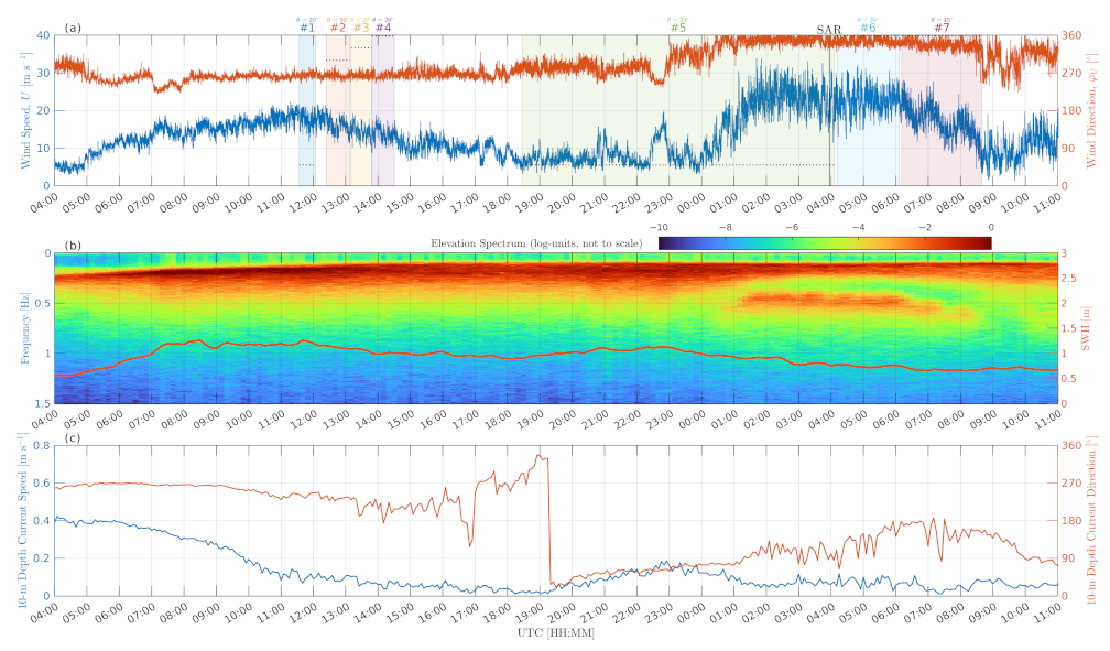
2.1. Experiment Site

The measurements presented in this study were taken from the Black Sea research platform (Figure 1d) during 24–25 October 2018. This platform is located seaward of the southern slope of the Crimean mountains, approximately 600 m offshore. In cold seasons, northerly katabatic drainage (bora) winds periodically develop, carrying high-density cold air from higher elevations over the Crimean Mountain plateau down its southern slope. At the platform location, local bora winds are topographically amplified in a coastal mountain canyon that acts as a tunnel (Figure 1b).
Such harsh conditions were observed during the experiment days. A Sentinel-1A Synthetic Aperture Radar image (SAR) taken at 03:57UTC on 25 October 2018 (Figure 1a) clearly indicates wind intensification (increased cross-section) over the coastal area, even in the anticipated mountain shadow zone. As typical bora wind is highly temporally variable and blows in gusts, a sample instantaneous imagery may not capture the peak of the wind event at each particular location. In fact, Figure 1a does not capture a gap-like wind jet over the platform, in contrast to numerous jets captured west of the platform. Based on our measurements, wind speed at the platform decreased to U 20 m s 1 during this Sentinel-1A overpass, but experienced periodical amplifications up to about 30 m s 1 in approximately 10 min cycles. At the platform location, the fetch of offshore wind-generated waves is about X 800 m. In our experience, for such short fetches and strong winds (young waves with dimensionless fetch, x = g X / U 2 10 ), spray clouds start developing over the surface when wind speed reaches 20–25 m s 1 (Figure 1c).

2.2. Instruments

For these experiments, a continuous wave Ka-band (37.5 GHz) Doppler radar was used [23]. It is equipped with a pair of identical conical horn antennas, one for transmission and one for receiving. The transmitted wave has mixed polarization while the receiver splits the incoming wave into vertical and horizontal polarization components. In this hybrid polarization mode, the received wave consists of like- and cross-polarized components. For regular sea surface backscattering, the latter component is much weaker in magnitude than the former component, and our radar measurements can be considered as dual-co-polarized measurements (see also Appendix B in [23]). For the present high wind measurements, with possibly larger volume backscattering from spray clouds, the effect of cross-polarization contamination will be discussed.
Wind speed was measured by a cup anemometer installed on top of the platform mast. The observed 23 m height wind speed was converted to the standard 10 m height neutral wind speed using the COARE 3.0 bulk parameterization [38]. Sea currents were measured by a propeller current meter installed at 10 m depth. Wave measurements were performed by conductive wire wave gauges, mounted at the vertices of a triangle with 5.31 m, 11.63 m, and 15.48 m sides [39]. Two-dimensional (2-D) directional frequency spectra were estimated using a standard approach, with north–south and east–west wave slopes calculated from instantaneous triangle inclinations and wave elevations taken from one of the wires [40,41].

2.3. Data Records

This experiment includes seven radar records collected at different look geometries and strongly varying winds (Figure 2a). During the initial period, the wind was westerly, with speed varying from 10 to 20 m s 1 . This was followed by an abrupt switch to strong offshore northerly wind with speed increasing up to 33 m s 1 . Currents at 10 m depth were below 0.2 m s 1 during the entire experiment (Figure 2c).
During the initial measurement period starting at 04:00UTC on 24 October 2018 (Records #1–4, Figure 2a), the wind wave spectrum had a single peak corresponding to predominantly westerly winds. The significant wave height (SWH) varied from 0.8 to 1 m with a rather stable wave peak frequency of about 0.2 Hz. At these conditions, four 30 min radar records were collected at low incidence angle, θ = 20 , and different azimuths.
After 23:00UTC on 24 October 2018, the wind direction started turning northerly with wind speed increasing to 30 m s 1 . This wind transition period was fully captured by the 9.5-h long Record #5, also collected at θ = 20 . As a result of wind direction change, the surface wave spectrum became bi-modal, with a residual gradually decaying 0.2-Hz wave system propagating from the west and a 0.5-Hz peak corresponding to ≈1-km fetch-limited wind waves propagating from the north (Figure 2b).
On the morning of 25 October 2018, the radar look azimuth was changed to upwind (Record #6). Next (Record #7), the incidence angle was increased to θ = 45 (also upwind) to capture the radar backscattering during the northerly wind gradual decay period.

2.4. General Definitions

Doppler radar data are computed from in-phase, I, and quadrature, Q, signal components sampled at 40 kHz for each (VV and HH) polarization. These raw signals yield “instantaneous” radar characteristics which are estimated from Doppler frequency spectra computed over consecutive 0.2-s intervals, S ( f d , t ) = | FFT ( I + i Q ) | 2 , where FFT is the Fourier transform. Integral characteristics of S ( f d , t ) are defined via its zeroth and first moments,
m 0 = S ( f d , t ) d f d , m 1 = f d S ( f d , t ) d f d
Doppler spectrum variance, m 0 , is a measure of received signal power. The Normalized Radar Cross-Section (NRCS), σ 0 , of the sea surface is estimated from m 0 multiplied by the known calibration coefficient and divided by the effective footprint area. The calibration coefficient is obtained from calibration measurements conducted with known backscattering targets [23].
The Doppler centroid frequency (also referred to as DC), f D = m 1 / m 0 , is related to the line-of-sight Doppler centroid velocity, V D = λ r / 2 · f D , where λ r = 0.8 cm is the radar wavelength. For our notations, positive/negative Doppler centroid frequency shifts, f D , correspond to approaching/moving away targets, respectively.

3. Sea Surface Cross-Section

3.1. Sea Spray Signatures

Signatures of sea spray in instantaneous Doppler spectra, S ( f d , t ) can be well identified. As a typical example, a part of Record #7 collected at θ = 45 is shown Figure 3. The spectrum can be speculatively partitioned into a low Doppler frequency, f d , “core”, associated with orbital motions of surface waves ( | V d | < 2 m s 1 ), and high | f d | transient tails, largely associated with radar signal spikes (mostly positive for upwind look geometry). Most of these spikes can also be associated with peaks in the “core” and/or wave breaking events (see more examples in the dedicated study [42]). However, some events occur independent of wave characteristics within the radar footprint. These latter events are likely produced by spray clouds generated upstream of the radar footprint.
For further insights, we select data with stable northerly wind direction and varying wind speed (Records #5 from 01:00UTC, #6, and #7). Instantaneous Doppler spectra are then averaged over different wind speed intervals (Figure 4), to illustrate some wind-dependent high-frequency Doppler spectrum features. The upper limit of the observed line-of-sight Doppler velocities is about 10 m s 1 (based on the radar signal-to-noise characteristics) or about 14 m s 1 (if converted to ground range speed). In our opinion, the only explanation for such high Doppler velocities is sea spray clouds embedded in the airflow. Regardless of polarization and incidence angle, the “tail” spectrum level is 3–4 orders of magnitude lower than the “core” spectrum level. Thus, though the spray contribution can be distinguished in Doppler spectra due to faster propagation speed, its net NRCS contribution is apparently negligible, at least at observed winds, U < 33 m s 1 .
The mean NRCS wind dependencies (Figure 5) do not explicitly exhibit any specific features, suggesting a backscattering regime change at strong winds. Mean NRCS dependencies are qualitatively similar to the background Ku-band geophysical model functions (GMF) derived from the Tropical Rainfall Measurement Mission (TRMM, the closest θ = 18 is used, see the bottom curve in their Figure 7 [30]) and NSCAT4 [43,44] satellite data. The TRMM GMF possibly suggests a noticeable NRCS decrease for U > 35 m s 1 , i.e., wind speeds exceeding our observation range. In general, this behavior is in line with the often-reported co-polarized backscatter saturation, possibly due to a wind stress attenuation at strong winds [45,46,47,48,49].
Our data are thus consistent with the background Ku-band GMF at low incidence angles, θ = 20 , for which strong wind speed dependence is not expected (Figure 5a,b,d,e). Our former NRCS parameterization (Ka-band Dual Polarization Model, KaDPMod, [23]) built on the same instrumental setup, but using more common wind conditions, U < 18 m s 1 , agrees well with the present dataset at strong winds, U > 10 m s 1 . The change of radar-to-wind azimuth (compare left and middle columns in Figure 5) does not significantly alter the NRCS wind dependence.
At larger incidence angles, θ = 45 (Figure 5c,f), the observed NRCS starts to be more wind-dependent, but stronger discrepancies are found compared to the Ku-band NSCAT4 GMF. In contrast to the NSCAT4 GMF, the observation data demonstrate a NRCS saturation tendency, starting at U > 25 m s 1 . The KaDPMod GMF does not reproduce these high wind observations well, because its wind dependence is fitted by a power function, σ U n , based on weaker wind data, U < 18 m s 1 . Alternatively, the observed NRCS at θ = 45 is fit with a second-order polynomial function, σ dB = A · U dB 2 + B · U dB + C , where σ dB and wind speed, U dB , are in dB-units, X dB = 10 log 10 X (see Figure 5c,f, green dashed lines).

3.2. NRCS Decomposition

The last Record #7 (see Figure 2a) offers a unique opportunity to separate different backscattering components in changing wind speed conditions. Providing that the fetch is limited at the northerly wind direction, the wind waves should rapidly adjust (in minutes) to wind changes. Thus, this 2.5-h-long Record #7 can be treated as the one composed from quasi-stationary samples of fetch-limited wind waves at different wind speeds.
First, we focus on the observed polarization ratio (PR), P  = σ 0 hh / σ 0 vv , a parameter directly reflecting the partition between polarized and non-polarized backscattering components. A small value of PR, P < 1 (or P < 0 dB), indicates a dominance of the resonant Bragg backscattering mechanism, while PR values approaching 1 (or 0 dB) suggest a dominance of the non-polarized (NP) backscattering mechanism. The latter mechanism generally results from quasi-specular reflection, either from a regular (non-breaking) surface at low incidence angles or a steep wave breaking surface (at larger incidence angles). At θ = 45 , the probability of regular specular reflections is quite small, thus the NP backscattering component can be fully attributed to wave breaking events.
Record #7 radar data are shown in Figure 6, including VV and HH NRCS in Figure 6a (also shown in Figure 5c,f) and PR in Figure 6b. These observation data are compared with the following GMFs and models:
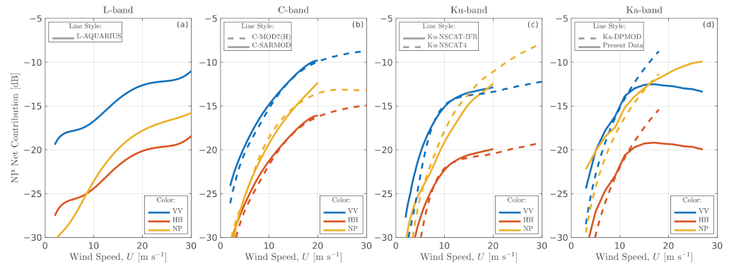
  • Ka-DPMOD, the Ka-band dual-co-polarized GMF based on data obtained with the same experiment setup as in the present study;
  • Ka-TSM, the two-scale (TSM) resonant Bragg model based on the radar imaging model (RIM) [50].
The above Ka-band estimates are augmented by empirical GMFs in other microwave bands to evaluate differences due to radar wavelength:
  • L-AQUARIUS, L-band (1.4 GHz) GMF inferred from Aquarius scatterometer data [51];
  • C-SARMOD, C-band (5.255 GHz) GMF based on joint VV and HH data from Envisat Advanced SAR (ASAR), Radarsat-2, and Sentinel-1 SARs [52] for θ 42 ;
  • C-MOD7(H), a combination of C-band CMOD7 (for VV polarization, [53]) and CMODH (for HH polarization, [54]) GMFs based on Envisat ASAR, Radarsat-2, and Sentinel-1 data for θ 42 ;
  • Ku-NSCAT-IFR, Ku-band GMF developed by the French Research Institute for Exploitation of the Sea (IFREMER) for NSCAT scatterometer data [55];
  • Ku-NSCAT4, Ku-band GMF (version 4) developed by the Royal Netherlands Meteorological Institute (KNMI) for NSCAT scatterometer data [44].
In line with previous studies [37,50,56,57], the observed PR ≈ −2 dB apparently exceeds TSM values, PR ≈ −7 dB (Figure 6b). Noticeably, empirical GMFs in Figure 6b suggest that PR decreases for longer radar wavelengths. However, its wind speed behavior is less obvious. While most of the GMFs in Figure 6b suggest that HH/VV ratio increases for U > 10 m s 1 (in line with expected stronger NP component contribution due to wave breaking intensification), the CMOD7(H) and KaDPMod suggest a decrease. This different behavior may be related to the way they were derived. In particular, the CMOD7(H) is a combination of independent VV and HH GMFs, which may have affected their ratio, i.e., the PR. In comparison to other GMFs, the KaDPMod is applicable in a relatively narrow wind speed range, U < 18 m s 1 , which may affect its wind speed dependencies. For U 12 m s 1 , the observed Ka-band PR fit closely follows the Ku-NSCAT4 PR.
An interesting feature of the observed PR wind dependency is the presence of a local minimum at about U = 10 m s 1 (Figure 6b). A similar PR minimum is also present in both Ku-band GMFs but at lower wind speed, U = 7 –8 m s 1 . For longer radar wavelengths (C- and L-bands), such minimum in PR wind dependence cannot be firmly identified.
To explain possible origins of the minimum in PR wind dependence, the NRCS is decomposed as a sum of polarized (Bragg) and NP components following [55,58],
σ 0 pp = σ br pp + σ np ,
where σ br pp is the resonant Bragg backscattering component described by a two-scale composite NRCS model. Given that both polarization NRCS, σ 0 vv and σ 0 hh , and theoretical Bragg polarization ratio, P br = σ 0 hh / σ 0 vv , are all known, the NP backscattering component can be estimated as,
σ np = σ 0 vv Δ σ 0 1 P br ,
where Δ σ 0 = σ 0 vv σ 0 hh = σ br vv σ br hh is the measured polarization difference (PD) and P br is estimated using the simplified RIM (see Appendix A of [50] for details).
Equation (3) provides estimates of the non-polarized (NP) backscattering component from the σ 0 vv , σ 0 hh , and Bragg polarization ratio, P br = σ br hh / σ br vv . If applied to the known empirical GMFs and the present Ka-band radar measurements, the results display different wind dependencies in different radar bands (Figure 7). In the L-band, the polarized (PP = VV, HH) contribution grows monotonically with wind for both polarizations. In the Ka-band, a tendency for PP saturation and further decrease at U > 10 –12 m s 1 is detected. To a lesser extent, the tendency for PP saturation is also present in the C- and Ku-bands. In the Ku- and Ka-band, the NP shows a weaker tendency for saturation in contrast to the PP and, thus, can retain some wind sensitivity at strong winds.
At moderate winds, U < 10 m s 1 , the NP is comparable in magnitude with the HH in the L-band, but its relative contribution increases systematically with decreasing radar wavelength and reaches the level of VV component in the Ku- and Ka-band at U 15–20 m s 1 (Figure 7). These changes are better seen when the relative NP contribution, σ 0 np / σ 0 pp , is explicitly shown (Figure 8). For instance, at U 15 m s 1 , our Ka-band data, as well as Ku-NSCAT4 GMF have the relative NP contribution of ≈50% (80%) for VV (HH) polarization, respectively. At U 30 m s 1 , this proportion increases to ≈70% (90%).
Equation (3) can also be seen as an explicit relationship between the relative NP contribution, σ 0 np / σ 0 pp , and the polarization ratio, P = σ 0 hh / σ 0 vv . As the Bragg TSM PR, P br = σ br hh / σ br vv , in (3) only weakly varies with wind speed (through the wind speed dependence of mean-square slope of long modulating waves, see black line in Figure 6b), the relative NP contribution should have the wind dependence very similar to that of PR, including the local minimum at U 10 m s 1 .
Thus the observed PR behavior (Figure 6b) can be attributed to specific balances between polarized and NP backscattering components. At light winds ≈4–5 m s 1 , the Bragg contribution is not strong enough to dominate the NP. Speculatively, this NP component might arise due to micro-scale wave breaking and steep features with very rare but strong quasi-specular reflections. As the wind increases to moderate speeds ≈10 m s 1 , the Ka-band polarized Bragg component grows rapidly and, importantly, faster than the wave breaking NP contribution, which decreases the PR in this wind speed range. The difference in wind growth rates is intuitively understood from the fact that resonant Bragg waves are short ( λ = 5.7 mm in the Ka-band at θ = 45 ), and thus respond faster to wind than waves responsible for (micro-scale) wave breaking ( λ 0.1 m) [59,60,61]. This hypothesis is indirectly supported by the fact that the growth rate of polarized components decreases and the local minimum of PR curve shifts towards lower winds (or even is not present) for longer radar, thus Bragg, wavelengths (Figure 6b). With further wind speed increase above 10–12 m s 1 , the Bragg polarized component starts saturating while the NP wave breaking component keeps growing (Figure 7d). At even stronger winds, the NP contribution dominates and the PR gradually increases to 0 dB.
The NRCS decomposition, Equation (2), also allows us to estimate the short wind wave spectrum at Bragg wavenumber. Indeed, the NP is canceled out by taking the polarization difference. Then, disregarding the hydrodynamics modulation component and applying the two-scale Bragg model [50,62,63,64],
σ br pp = σ 0 br pp 1 + g pp ζ 2 ¯ ,
σ 0 br pp = π | G pp 2 | B ( k br ) ,
G vv = ( ϵ 1 ) ( ϵ + ( ϵ 1 ) sin 2 θ ) cos 2 θ ( ϵ cos θ + ϵ sin 2 θ ) 2 sin 2 θ ,
G hh = ( ϵ 1 ) cos 2 θ ( cos θ + ϵ sin 2 θ ) 2 sin 2 θ ,
g pp = 1 2 σ 0 br pp 2 σ 0 br pp θ 2 .
the polarization difference, PD = Δ σ 0 , is determined only by the radar look geometry, mean-square slope of long waves, and Bragg wave curvature spectrum, B 0 ( k br ) = k 4 S ( k br ) :
Δ σ 0 = π B ( k br ) ( Δ ( | G pp 2 | ) + Δ ( | G pp 2 | g pp ) ζ 2 ¯ ) ,
where Δ ( x ) = x vv x hh is the PD operator, G pp and g pp are the geometric coefficients (with cross-tilt contribution omitted for g hh , see Figure 5 in [50]), ϵ is the complex sea water dielectric constant estimated using [65] for 18 C temperature, 18 psu salinity, and 37.5 GHz electromagnetic frequency, ζ 2 ¯ is the mean-square slope (mss) of modulating waves in the incidence plane, k br = 2 k r sin θ is the Bragg wave vector, k r is the radar electromagnetic wave vector, and B ( k br ) = ( B 0 ( k br ) + B 0 ( k br ) ) / 2 is the folded curvature spectrum reflecting that Bragg components directed towards and away from radar both contribute.
Wind dependence of the folded curvature spectrum, B ( k br ) , estimated from Equation (9) and shown in Figure 9a is similar to that of polarized backscatter components in Figure 7. The folded curvature spectra estimated in the four radar frequency bands are interpolated in wavenumber space by polynomial splines (Figure 9b). The resulting spectra have stronger wind dependence in the Ku- and C-bands and display a tendency to saturate at U > 15–20 m s 1 .
Errors of curvature spectral retrieval depend in part on the uncertainty of modulating wave mss and the measurement accuracy of the NRCS (PD). It is usually postulated that “modulating” waves are separated from “short-scale” waves by a so-called dividing wavenumber, k d = k r / d , with d 3 to 4. To account for uncertainties of the ζ 2 ¯ , several estimates were employed. These include the Phillips spectrum model [66], ζ 2 ¯ = 4.6 · 10 3 ln ( k d / k p ) / 2 , with equal up- and cross-wind mss components and peak wavenumber, k p = g / U 2 or k p = 1 rad m 1 (the latter was observed in fetch-limited conditions at northerly offshore wind), as well as the Cox and Munk [67] clean surface and slick-covered empirical mss parameterizations. Excluding the Cox and Munk clean surface parameterization, which apparently overestimates the mss of modulating waves, the above range of mss estimates results in only <0.3 dB uncertainty in the final curvature spectrum estimates. For “typical” radar measurement conditions, the NRCS (PD) error is about 1–2 dB and thus it dominates the uncertainty of wave curvature spectrum estimate (Figure 9a).

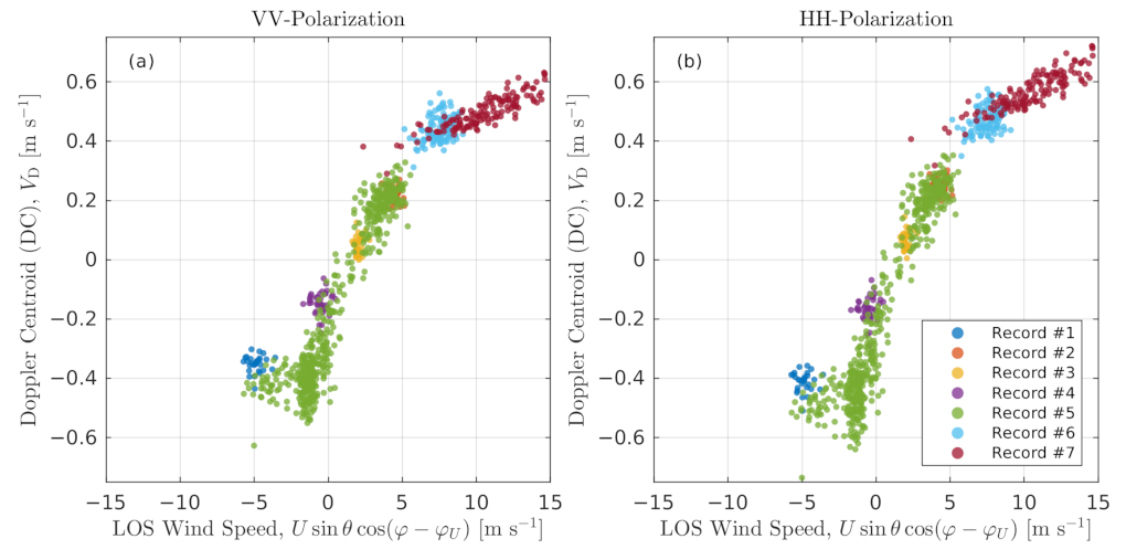
4. Sea Surface Doppler Centroid

The Doppler spectrum centroid (DC) is the main parameter for sea surface current retrieval from Doppler scatterometer measurements [68,69,70,71,72,73,74,75,76]. In our previous study based on the same experimental setup, we have demonstrated [26] the possibility of sea surface current retrieval from DC measurements using the radar Modulation Transfer Function (MTF) approach [25,77,78] for “regular” winds, U < 15 –18 m s 1 , and long fetches, ≥100 km. The present data provide a way to check if this approach is still applicable at stronger winds, ≈20–30 m s 1 , and limited fetches, ≈1 km. From the above Doppler spectra analysis (Figure 4), no essential sea spray impacts are expected, but other factors, including MTF applicability at strong wind/short fetches, need further examination.
For space/air-borne scatterometer set up with a large ground footprint size, the DC is “automatically” measured when the footprint size exceeds a few peak wavelengths, i.e., surface waves are not spatially resolved. For tower-based measurements, the effective radar footprint size is several meters long and wide (see Appendix A, Figure 14 in [25] for details), and energy-containing surface waves (typically 40 m, 5-s period at the platform site) are resolved. In this case, the DC is based on temporal rather than spatial averaging. In terms of instantaneous Doppler spectra, S ( f d , t ) , and ignoring possible non-ergodicity of the wave field, the DC reads,
V D = f d S ( f d , t ) d f d d t S ( f d , t ) d f d d t ,
where time averaging is performed over an interval sufficiently exceeding the peak wave period. We select 1 min averaging interval corresponding to ≈12 or more characteristic peak wave periods.
The DC reflects the footprint-averaged sea surface motion that is mainly governed by waves and currents [56,69,79], which are entirely, or in part, forced by winds. As a first guess and following [69], the measured DC is compared in Figure 10 with the line-of-sight (LOS) wind vector projection, U LOS = U sin θ cos ( φ φ U ) . There is a visually good correlation between the two, but with different slopes (or gain factors in terms of [22]) for different incidence angles (compare Record #7 data collected at θ = 45 with other records collected at θ = 20 ). Firstly, this close correlation is explained by weak non-wind-driven background currents (see Figure 2c for 10 m current speed) and, secondly, by a close relationship between wind and waves at the experiment site. The exception from this is seen for a downwind (negative) part of Record #5 (Figure 10, green dots), for which the relationship between the DC and LOS wind velocity differs for 5 m s 1 < U LOS < 0 m s 1 . This part of Record #5 was acquired during an abrupt switch in wind speed and direction between 22:20 and 23:00UTC on 25 October 2018 (Figure 2) at virtually constant wave height and direction.
To achieve deeper insights into the physics of Doppler imaging mechanisms, the DC is further analyzed in terms of the MTF-based Ka-band Doppler (KaDOP) model [26], which is briefly summarized below.

4.1. The KaDOP Approach

In the KaDOP, the DC is represented as a sum of surface currents (term 1), Bragg wave velocity (term 2), and wave-induced Doppler velocity (WIDV, term 3),
V D = v dr sin θ cos ( φ r φ dr ) + v sc sin θ + g 1 Re { M ( θ , φ , U ) G ( θ , φ ) } ω 3 S ( ω , φ ) d ω d φ ,
where v dr and φ dr are the surface current speed and direction, g is the gravity acceleration, ω = 2 π f is the radial wave frequency, φ r is the radar azimuth, M ( θ , φ , U ) is the MTF empirical parameterization [25], G = cos ( φ r φ ) sin θ i cos θ is the geometrical coefficient projecting wave orbital velocity onto the radar LOS and M · G is the LOS MTF, and v sc is the inherent scatterer velocity approximated by Bragg wave phase velocity [26].
The surface current velocity, v dr , is decomposed into a sum of a background current (from current meter measurements at 10 m depth), which may not be related to local winds, and a wind-driven current shear in the upper 10 m layer. Following [26], the latter is estimated as 1.5 % · U .
The WIDV is the most challenging contribution. Firstly, it is not intuitive in contrast to surface currents and inherent scatter velocity. Secondly, the WIDV can dominate over other terms of Equation (11) [76,80]. Next, two characteristic records are considered to demonstrate WIDV contribution in different environmental conditions and at different radar look geometry configurations, θ = 20 and θ = 45 . Without loss of generality, only VV data are presented, because HH data (not shown) show similar results.
For further analysis, the “direct” WIDV estimate, which is possible with our wave-resolving platform measurements, is also used. As shown in [13,81], the instantaneous Doppler velocity or the centroid of instantaneous Doppler spectrum,
v ˜ ( t ) = f d S ( f d , t ) d f d S ( f d , t ) d f d ,
is a measure of “pure” footprint kinematics. Therefore, the difference between the DC and the time-mean of this quantity, V D v ˜ ¯ , cancels out the surface current and the inherent scatterer velocity, and thus isolates the WIDV. However, the v ˜ is also contributed by waves not resolved by the radar footprint. Hence, the difference, V D v ˜ ¯ , accounts for WIDV contribution only from waves longer than the footprint size (2 m by 2 m at θ = 20 , and 2.5 m by 4 m at θ = 45 ).

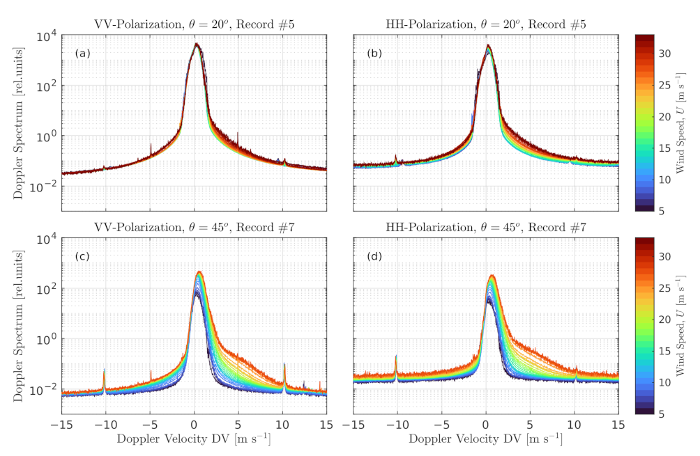
4.2. Small Incidence Angle (Record #5)

Record #5 (Figure 11) is remarkable due to the fully recorded wind direction turning event, with short interruptions during two strong rain events. During this entire record, the radar was oriented downwind relative to westerly winds. During the first part of Record #5 collected at westerly winds (before 00:00UTC on 25 October 2018), the combined DC contribution from background current, Bragg velocity, and wind drift is ≈25% of the total DC (Figure 11a, compare green and blue lines). Hence, the remaining ≈75% is produced by the WIDV. After the wind direction switch into the northerly direction (after 00:00UTC on 25 October 2018), the partitioning changes to ≈50/50% due to changes in wave regime and relative radar azimuth (crosswind). Notice that combined contribution from 10 m currents, wind drift, and Bragg velocity changes its sign but remains ≈0.1 m s 1 in magnitude. The measured WIDV estimated as the difference between the total measured DC and the sum of background current, wind drift, and Bragg velocity is shown by the blue line in Figure 11c. An alternative “direct” estimate of the WIDV, V D v ˜ ¯ , is consistent with the former estimate but has a smaller magnitude as it only accounts for waves resolved by the radar footprint.
As illustrated in Figure 11a, the WIDV is the dominant part of the DC. Hence, inverting the DC into the surface current requires precise knowledge of the WIDV. The present dataset provides a useful testbed to evaluate KaDOP model [26] performance. First, the KaDOP is evaluated using the observed frequency-angular wave spectrum concurrently measured by the triangle wave gauge array. This estimate is apparently below the measured WIDV magnitude for the downwind part of Record #5 and even has wrong WIDV sign for the crosswind part of Record #5 (Figure 11c, purple line). These discrepancies are explained by the geometry of the wave gauge triangle which has a too-long base, ≈10 m, that significantly limited in-situ wave measurements. While gauge-measured wave frequency spectra are limited by the sampling rate, f < 2 Hz, their angular-frequency wave spectra are cut off at λ 20 m or f 0.3 Hz (Figure 12a), which results in WIDV underestimation for the westerly wind part of Record #5. During the northerly part of Record #5, the very young (hence short) offshore waves are not resolved by the triangle array that results in erroneous spectra estimates for this wave system (Figure 12b), and thus deficient WIDV estimates.
For qualitative demonstrations, we simulate the high frequency part of wave spectra, f > 0.3 Hz, using the modified JONSWAP spectrum [82], with wave direction defined by instantaneous wind, and smoothly merge it with the measured low-frequency part, f < 0.3 Hz. Wave age and spectrum level parameters of the simulated part are selected to fit its peak frequency and elevation variance with those from observed 1D frequency wave spectra. When these simulated wave spectra are used in Equation (11), the KaDOP WIDV estimates improve, with the correct sign in the cross-wind part of Record #5 (green line in Figure 11c).
Nevertheless, there remains one noticeable discrepancy between observed and simulated WIDV between 22:00 and 23:00 UTC (compare observations, blue line, and simulations, green line, in Figure 11c). From our simulations (not shown), this discrepancy wiggle is related to abrupt and substantial changes in wind direction accompanying its turning from westerly to northerly winds. Using instantaneous wind direction as a proxy for wave direction (even at f > 0.3 Hz) may not be appropriate during such abrupt changes. In general, this confirms the conclusions of Miao et al. [75] and Martin et al. [76] that observed wave spectra (rather than wind-based parameterizations) are key for accurate WIDV simulations, especially in complex wave conditions.

4.3. Moderate Incidence Angle (Record #7)

For moderate incidence angles, θ = 45 , (Record #7, Figure 13), the line-of-sight DC increases up to ≈0.6 m s 1 due in part to larger projection factor, sin θ . The gradual wind decay during Record #7 is reflected in the corresponding DC decay. Noticeably, DC variations better correlate with wind variations (Figure 13) compared to the θ = 20 case (Figure 11). The magnitude of surface current and scatter velocity combined contribution (first two terms in Equation (11)) is below the observed DC, with the difference equal to the WIDV (green and blue lines in Figure 13a). The WIDV (Figure 13c) is smaller in magnitude than for θ = 20 due to the MTF magnitude decrease with the incidence angle [22,25]. An alternative WIDV estimate, V D v ˜ ¯ , is almost zero because the dominant 0.5-Hz fetch-limited waves are not well resolved by the radar footprint (≈4 m). Eastward swell also present in the scene comes obliquely to the northward radar look direction and thus does not affect the DC significantly (Figure 12c,d).
If wave gauge array measured 2D directional wave spectra are used in Equation (11) for WIDV estimate, the KaDOP prediction is about zero (Figure 13c, purple line) because such young, short waves are not resolved by the triangle array with relatively long (≈10 m) base. If this unresolved part of the wave spectrum is simulated based on the JONSWAP parameterization (Figure 12d), the WIDV fits the measurements better, although not perfectly (Figure 13c, green line). The remaining discrepancy may be attributed to uncertainties in surface currents (which are estimated from measured 10 m currents but parameterized 0–10 m current shear, 1.5 % · U ) and simulated wave spectra.
It could be noted that the relative WIDV contribution decreases for slanted look geometries due to smaller MTF magnitude and related weaker NRCS modulations. The DC becomes more closely governed by the sum of surface current and Bragg contributions as the incidence angle increases.

5. Discussion

The presented results, both for backscatter intensity and Doppler shifts, suggest that sea spray contribution does not significantly affect the average NRCS and DC, at least for θ 45 and U < 33 m s 1 . Although sea spray signatures are several orders of magnitude weaker than sea surface radar signatures, they can be isolated in the Doppler spectrum due to faster Doppler speed. This can be potentially important for the remote sensing of sea spray parameters but is out of scope of this study.
These measurements are collected using a hybrid polarization radar, with VV and HH signals potentially contaminated by cross-polarized HV and VH signals, respectively. As shown before, such contamination is not significant for regular sea surface backscattering (Appendix B of [23]), but may be an issue for volume backscattering due to its expected depolarization effects. Although potential volume backscattering impacts can not be directly estimated from our data, it is speculated that they should not affect our final results based on the following reasons. First, this is indirectly confirmed by quite good correspondence between our data and Ku-band GMFs (Figure 5, Figure 6, Figure 7 and Figure 8). Second, the Ka-band precipitation radar simulations and measurements [83] suggest that the linear depolarization ratio due to multiple scattering is about −20 to 15 dB if the penetration depth in a heavy rain cloud is less than 1 km. In our case, the penetration depth is determined by the radar beam size of several meters, for which the depolarization effect should be negligible. Third, even if one assumed the depolarization ratio equal 1 (all energy backscattered from spray volume illuminated by co-polarized radar radiation is backscattered as randomly polarized signal due to the multiple scattering), then our hybrid measurement would be overestimated by a factor of two at each polarization, VV + HV, and HH + VH. This would also imply that spray signatures in measured Doppler spectra (spectrum tails) are over estimated by a factor of two, and the uncontaminated VV and HH are even weaker.
Another indirect evidence of weak sea spray contribution is the fact that our DC model, KaDOP [26], derived for regular non-spray conditions, can be extrapolated to gale force winds without invoking additional modifications. Even at strong winds, the conventional radar MTF approach is sufficient to evaluate the WIDV.
The presence of multiple wave systems may also affect the DC, which was demonstrated for low-frequency swell contribution [26]. However, a potentially more important contribution is related to the high frequency part of wave spectra, as it can be anticipated from the fact that the WIDV is governed by the third moment of the frequency elevation spectrum, a Stokes drift-like term, Equation (11). This is confirmed by the present study demonstrating the dramatic difference between DC predictions using wave spectra with cut-off high frequency part (based on wave array measurements) and those with high-frequency part restored from observed wind velocity (measurements+simulation). Thus, local wind variability may be important for DC prediction, for which a proper description of the short-wave part of wave spectra is required.

6. Conclusions

This paper presents field measurements of the sea surface radar backscatter cross-section and Doppler centroid in the Ka-band collected at rather strong (up to 33 m s 1 ) wind speeds with distinct events of spray formation above the sea surface. Water droplet propagation within the radar beam causes the volume scattering and high-frequency signatures in the Doppler spectrum with Doppler velocities up to or even exceeding 10 m s 1 . However, the high-frequency tail spectral energy is 3 to 4 orders of magnitude weaker than the spectral energy of the signal backscattered from the sea surface. Hence, the spray contribution to the total NRCS observed in our experiment is negligible.
Using the previously developed NRCS decomposition approach [55,58] and this paper’s co-polarized radar measurements, polarized Bragg-like and non-polarized (NP) radar backscatter components are assessed in a wide range of wind speeds and at similar wave conditions. Several empirical radar geophysical model functions (GMFs) developed for the L-, C-, and Ku-bands are used to estimate the short-scale wind wave spectrum. Previously, using the same experimental setup but for data collected at weaker wind speeds, U < 15 m s 1 , a decrease in NP relative contribution with growing wind speed has been reported [23]. This feature is confirmed with the present data, which also show that NP contribution starts increasing at U > 15 m s 1 , thus leading to a local minimum in the relative NP contribution. Empirical GMFs show that such local minimum in the relative NP contribution, thus in the polarization ratio, is also present in other bands. Although the relative contribution of breaking wave backscattering component increases in strong winds, the short-scale roughness spectrum (hence Bragg-like polarized backscatter) saturates at U > 15 m s 1 . The balance between polarized and non-polarized backscattering components governs the wind speed dependence of the NRCS, which is still not yet fully saturated for U < 30 m s 1 .
The Doppler spectrum centroid is dominated by “slow” surface rather than “fast” volume scattering. With several long records in hand, it is demonstrated how the conventional radar modulation transfer function (MTF) approach (adopted for the Doppler centroid estimation in the KaDOP model [26]) can be applied to changing wind and wave conditions. On average, the KaDOP model adequately represents sea surface radar measurements. However, the effect of rapid changes in wind and wave conditions cannot be represented well by this model without the precise knowledge of concurrent wave spectra.
This paper findings indicate that Doppler centroid prediction depends strongly on adequate knowledge of surface wave parameters rather than wind parameters. Although it is demonstrated for young offshore waves, similar wave conditions can be present in the open ocean under rapidly changing winds. This is especially important for small incidence angles, ≈ 20 , exhibiting stronger long-wave NRCS modulation and wave-induced Doppler velocity contribution. Thus, in contrast to traditional NRCS geophysical model functions that solely rely on wind speed for sea state representation, the Doppler radar modeling is expected to be more robust if wave information is directly used.

Supplementary Materials

The following supporting information can be downloaded at: https://www.mdpi.com/article/10.3390/rs14061348/s1, Video S1: The sea surface with spray clouds at 20–30 m/s wind speed observed during the experiment.

Author Contributions

V.N.K. and Y.Y.Y. conceived and designed the experiments; V.N.K., B.C. and S.A.G. provided the sea surface modeling; Y.Y.Y. performed the experiments, analyzed the data, and wrote the paper. All authors have read and agreed to the published version of the manuscript.

Funding

The data analysis and radar modeling performed in this work were supported by the Russian Science Foundation under Grant 21-17-00236 (https://rscf.ru/en/project/21-17-00236/, accessed on 6 March 2022). The field experiments are sponsored by the MHI RAS State Order (Goszadanie) 0555-2021-0004. Sea surface modeling approach is developed within the frame of the RSHU State Order (Goszadanie) 0763-2020-0005. SG was supported by the NASA Physical Oceanography.

Conflicts of Interest

The authors declare no conflict of interest.

References

  1. Fois, F.; Hoogeboom, P.; Le Chevalier, F.; Stoffelen, A. DOPSCAT: A mission concept for a Doppler wind-scatterometer. In Proceedings of the 2015 IEEE International Geoscience and Remote Sensing Symposium (IGARSS), Milan, Italy, 26–31 July 2015; pp. 2572–2575. [Google Scholar] [CrossRef]
  2. Bao, Q.; Lin, M.; Zhang, Y.; Dong, X.; Lang, S.; Gong, P. Ocean surface current inversion method for a Doppler scatterometer. IEEE Trans. Geosci. Remote Sens. 2017, 55, 6505–6516. [Google Scholar] [CrossRef]
  3. Miao, Y.; Dong, X.; Bao, Q.; Zhu, D. Perspective of a Ku-Ka dual-frequency scatterometer for simultaneous wide-swath ocean surface wind and current measurement. Remote Sens. 2018, 10, 1042. [Google Scholar] [CrossRef] [Green Version]
  4. Gommenginger, C.; Chapron, B.; Martin, A.; Marquez, J.; Brownsword, C.; Buck, C. SEASTAR: A new mission for high-resolution imaging of ocean surface current and wind vectors from space. In Proceedings of the EUSAR 2018, 12th European Conference on Synthetic Aperture Radar, Aachen, Germany, 4–7 June 2018; pp. 1433–1436. [Google Scholar]
  5. Ardhuin, F.; Brandt, P.; Gaultier, L.; Donlon, C.; Battaglia, A.; Boy, F.; Casal, T.; Chapron, B.; Collard, F.; Cravatte, S.; et al. SKIM, a candidate satellite mission exploring global ocean currents and waves. Front. Mar. Sci. 2019, 6, 209. [Google Scholar] [CrossRef] [Green Version]
  6. Rodríguez, E.; Bourassa, M.; Chelton, D.; Farrar, J.T.; Long, D.; Perkovic-Martin, D.; Samelson, R. The winds and currents mission concept. Front. Mar. Sci. 2019, 6, 438. [Google Scholar] [CrossRef]
  7. Rodriguez, E. On the optimal design of doppler scatterometers. Remote Sens. 2018, 10, 1765. [Google Scholar] [CrossRef] [Green Version]
  8. Masuko, H.; Okamoto, K.; Shimada, M.; Niwa, S. Measurement of microwave backscattering signatures of the ocean surface using X-band and Ka-band airborne scatterometers. J. Geophys. Res. (Oceans) 1986, 91, 13065–13084. [Google Scholar] [CrossRef]
  9. Plant, W.J.; Terray, E.A.; Petitt, R.A.; Keller, W.C. The dependence of microwave backscatter from the sea on illuminated area: Correlation times and lengths. J. Geophys. Res. (Oceans) 1994, 99, 9705–9723. [Google Scholar] [CrossRef]
  10. Vandemark, D.; Chapron, B.; Sun, J.; Crescenti, G.H.; Graber, H.C. Ocean wave slope observations using radar backscatter and laser altimeters. J. Phys. Oceanogr. 2004, 34, 2825–2842. [Google Scholar] [CrossRef]
  11. Nekrasov, A.; Hoogeboom, P. A Ka-band backscatter model function and an algorithm for measurement of the wind vector over the sea surface. IEEE Geosci. Remote Sens. Lett. 2005, 2, 23–27. [Google Scholar] [CrossRef]
  12. Walsh, E.J.; Wright, C.W.; Banner, M.L.; Vandemark, D.C.; Chapron, B.; Jensen, J.; Lee, S. The southern ocean waves experiment. Part III: Sea surface slope statistics and near-nadir remote sensing. J. Phys. Oceanogr. 2008, 38, 670–685. [Google Scholar] [CrossRef]
  13. Ermakov, S.A.; Kapustin, I.A.; Kudryavtsev, V.N.; Sergievskaya, I.A.; Shomina, O.V.; Chapron, B.; Yurovskiy, Y.Y. On the Doppler frequency shifts of radar signals backscattered from the sea surface. Radiophys. Quantum Electron. 2014, 57, 239–250. [Google Scholar] [CrossRef]
  14. Boisot, O.; Pioch, S.; Fatras, C.; Caulliez, G.; Bringer, A.; Borderies, P.; Lalaurie, J.C.; Guérin, C.A. Ka-band backscattering from water surface at small incidence: A wind-wave tank study. J. Geophys. Res. (Oceans) 2015, 120, 3261–3285. [Google Scholar] [CrossRef]
  15. Nouguier, F.; Mouche, A.; Rascle, N.; Chapron, B.; Vandemark, D. Analysis of dual-frequency ocean backscatter measurements at Ku- and Ka-bands using near-nadir incidence GPM radar data. IEEE Geosci. Remote Sens. Lett. 2016, 13, 1310–1314. [Google Scholar] [CrossRef] [Green Version]
  16. Rodriguez, E.; Wineteer, A.; Perkovic-Martin, D.; Gál, T.; Stiles, B.; Niamsuwan, N.; Rodriguez Monje, R. Estimating ocean vector winds and currents using a Ka-Band pencil-beam Doppler scatterometer. Remote Sens. 2018, 10, 576. [Google Scholar] [CrossRef] [Green Version]
  17. Marié, L.; Collard, F.; Nouguier, F.; Pineau-Guillou, L.; Hauser, D.; Boy, F.; Méric, S.; Peureux, C.; Monnier, G.; Chapron, B.; et al. Measuring ocean surface velocities with the KuROS and KaRADOC airborne near-nadir Doppler radars: A multi-scale analysis in preparation of the SKIM mission. Ocean Sci. Discuss. 2019, 2019, 1–52. [Google Scholar] [CrossRef]
  18. Ermakov, S.A.; Dobrokhotov, V.A.; Sergievskaya, I.A.; Kapustin, I.A. Suppression of wind ripples and microwave backscattering due to turbulence generated by breaking surface waves. Remote Sens. 2020, 12, 3618. [Google Scholar] [CrossRef]
  19. Mouche, A.A.; Chapron, B.; Reul, N.; Collard, F. Predicted Doppler shifts induced by ocean surface wave displacements using asymptotic electromagnetic wave scattering theories. Waves Random Media 2008, 18, 185–196. [Google Scholar] [CrossRef]
  20. Gairola, R.M.; Prakash, S.; Mahesh, C.; Gohil, B.S. Model function for wind speed retrieval from SARAL-AltiKa radar altimeter backscatter: Case studies with TOPEX and JASON data. Mar. Geod. 2014, 37, 379–388. [Google Scholar] [CrossRef]
  21. Fois, F.; Hoogeboom, P.; Le Chevalier, F.; Stoffelen, A. An analytical model for the description of the full-polarimetric sea surface Doppler signature. J. Geophys. Res. (Oceans) 2015, 120, 988–1015. [Google Scholar] [CrossRef] [Green Version]
  22. Nouguier, F.; Chapron, B.; Collard, F.; Mouche, A.; Rascle, N.; Ardhuin, F.; Wu, X. Sea surface kinematics from near-nadir radar measurement. IEEE Trans. Geosci. Remote Sens. 2018, 56, 6169–6179. [Google Scholar] [CrossRef]
  23. Yurovsky, Y.Y.; Kudryavtsev, V.N.; Grodsky, S.A.; Chapron, B. Ka-band dual copolarized empirical model for the sea surface radar cross section. IEEE Trans. Geosci. Remote Sens. 2016, 55, 1629–1647. [Google Scholar] [CrossRef]
  24. Yurovsky, Y.Y.; Kudryavtsev, V.N.; Grodsky, S.A.; Chapron, B. Low-frequency sea surface radar Doppler echo. Remote Sens. 2018, 10, 870. [Google Scholar] [CrossRef] [Green Version]
  25. Yurovsky, Y.Y.; Kudryavtsev, V.N.; Chapron, B.; Grodsky, S.A. Modulation of Ka-band Doppler radar signals backscattered from the sea surface. IEEE Trans. Geosci. Remote Sens. 2018, 56, 2931–2948. [Google Scholar] [CrossRef] [Green Version]
  26. Yurovsky, Y.Y.; Kudryavtsev, V.N.; Grodsky, S.A.; Chapron, B. Sea surface Ka-band Doppler measurements: Analysis and model development. Remote Sens. 2019, 11, 839. [Google Scholar] [CrossRef]
  27. Quilfen, Y.; Chapron, B.; Elfouhaily, T.; Katsaros, K.; Tournadre, J. Observation of tropical cyclones by high-resolution scatterometry. J. Geophys. Res. (Oceans) 1998, 103, 7767–7786. [Google Scholar] [CrossRef]
  28. Donnelly, W.J.; Carswell, J.R.; McIntosh, R.E.; Chang, P.S.; Wilkerson, J.; Marks, F.; Black, P.G. Revised ocean backscatter models at C and Ku band under high-wind conditions. J. Geophys. Res. (Oceans) 1999, 104, 11485–11498. [Google Scholar] [CrossRef]
  29. Fernandez, D.E.; Carswell, J.R.; Frasier, S.; Chang, P.S.; Black, P.G.; Marks, F.D. Dual-polarized C- and Ku-band ocean backscatter response to hurricane-force winds. J. Geophys. Res. (Oceans) 2006, 111. [Google Scholar] [CrossRef] [Green Version]
  30. Li, X.; Zhang, B.; Mouche, A.; He, Y.; Perrie, W. Ku-band sea surface radar backscatter at low incidence angles under extreme wind conditions. Remote Sens. 2017, 9, 474. [Google Scholar] [CrossRef] [Green Version]
  31. Goldstein, H. Sea echo. In Propagation of Short Radio Waves; Kerr, D.E., Ed.; IET: London, UK, 1947; pp. 481–571. [Google Scholar]
  32. Sharkov, E.A. Breaking Ocean Waves: Geometry, Structure and Remote Sensing; Springer: Berlin/Heidelberg, Germany, 2007. [Google Scholar]
  33. Raizer, V. Radar backscattering from sea foam and spray. In Proceedings of the International Geoscience and Remote Sensing Symposium, Melbourne, Australia, 21–26 July 2013; pp. 4054–4057. [Google Scholar] [CrossRef]
  34. Doviak, R.J.; Zrnic, D.S. Meteorological radar signal processing. In Doppler Radar and Weather Observations; Academic Press: San Diego, CA, USA, 1984; pp. 91–120. [Google Scholar]
  35. Kalmykov, A.I.; Kurekin, A.S.; Lementa, Y.A.; Ostrovskii, I.E.; Pustovoitenko, V.V. Characteristics of SFH scattering at breaking sea waves. Radiophys. Quantum Electron. 1976, 19, 923–928. [Google Scholar] [CrossRef]
  36. Plant, W.J. Microwave sea return at moderate to high incidence angles. Waves Random Media 2003, 13, 339–354. [Google Scholar] [CrossRef] [Green Version]
  37. Plant, W.J.; Keller, W.C.; Asher, W.E. Is sea spray a factor in microwave backscatter from the ocean? In Proceedings of the 2006 IEEE MicroRad, San Juan, PR, USA, 28 February–3 March 2006; pp. 115–118. [Google Scholar] [CrossRef]
  38. Fairall, C.W.; Bradley, E.F.; Hare, J.E.; Grachev, A.A.; Edson, J.B. Bulk parameterization of air sea fluxes: Updates and verification for the COARE algorithm. J. Clim. 2003, 16, 571–591. [Google Scholar] [CrossRef]
  39. Zapevalov, A.S.; Garmashov, A.V. Skewness and kurtosis of the surface wave in the coastal zone of the Black Sea. Phys. Oceanogr. 2021, 28, 414–425. [Google Scholar] [CrossRef]
  40. Longuet-Higgins, M.S.; Cartwright, D.E.; Smith, N.D. Observations of the directional spectrum of sea waves using the motions of a floating buoy. In Ocean Wave Spectra: Proceedings of a Conference; North Atlantic Oscillation Sciences; Prentice Hall: Hoboken, NJ, USA, 1961; pp. 111–132. [Google Scholar]
  41. Earle, M.D.; Brown, R.; Baker, D.J.; McCall, J.C. Nondirectional and Directional Wave Data Analysis Procedures. NDBC Technical Document 96-01, Stennis Space Center, 1996. Available online: www.ndbc.noaa.gov/wavemeas.pdf (accessed on 25 January 2022).
  42. Yurovsky, Y.Y.; Kudryavtsev, V.N.; Grodsky, S.A.; Chapron, B. Ka-band radar cross-section of breaking wind waves. Remote Sens. 2021, 13, 1929. [Google Scholar] [CrossRef]
  43. Wentz, F.J.; Smith, D.K. A model function for the ocean-normalized radar cross section at 14 GHz derived from NSCAT observations. J. Geophys. Res. (Oceans) 1999, 104, 11499–11514. [Google Scholar] [CrossRef]
  44. NSCAT-4 Geophysical Model Function. Royal Netherlands Meteorological Institute (KNMI). Available online: https://scatterometer.knmi.nl/nscat_gmf/ (accessed on 25 January 2022).
  45. Donelan, M.A.; Haus, B.K.; Reul, N.; Plant, W.J.; Stiassnie, M.; Graber, H.C.; Brown, O.B.; Saltzman, E.S. On the limiting aerodynamic roughness of the ocean in very strong winds. Geophys. Res. Lett. 2004, 31, L18306. [Google Scholar] [CrossRef] [Green Version]
  46. Kudryavtsev, V.N. On the effect of sea drops on the atmospheric boundary layer. J. Geophys. Res. (Oceans) 2006, 111. [Google Scholar] [CrossRef]
  47. Kudryavtsev, V.N.; Makin, V.K. Aerodynamic roughness of the sea surface at high winds. Bound.-Layer Meteorol. 2007, 125, 289–303. [Google Scholar] [CrossRef]
  48. Troitskaya, Y.I.; Sergeev, D.A.; Kandaurov, A.A.; Baidakov, G.A.; Vdovin, M.A.; Kazakov, V.I. Laboratory and theoretical modeling of air-sea momentum transfer under severe wind conditions. J. Geophys. Res. Ocean. 2012, 117. [Google Scholar] [CrossRef]
  49. Hwang, P.A.; Li, X.; Zhang, B. Coupled nature of hurricane wind and wave properties for ocean remote sensing of hurricane wind speed. In Hurricane Monitoring with Spaceborne Synthetic Aperture Radar; Li, X., Ed.; Series Title: Springer Natural Hazards; Springer: Singapore, 2017; pp. 215–236. [Google Scholar] [CrossRef]
  50. Kudryavtsev, V.; Hauser, D.; Caudal, G.; Chapron, B. A semiempirical model of the normalized radar cross-section of the sea surface 1. Background model. J. Geophys. Res. (Oceans) 2003, 108, C08054. [Google Scholar] [CrossRef] [Green Version]
  51. Meissner, T.; Wentz, F.J.; Ricciardulli, L. The emission and scattering of L-band microwave radiation from rough ocean surfaces and wind speed measurements from the Aquarius sensor. J. Geophys. Res. (Oceans) 2014, 119, 6499–6522. [Google Scholar] [CrossRef]
  52. Mouche, A.; Chapron, B. Global C-band envisat, RADARSAT-2 and Sentinel-1 SAR measurements in copolarization and cross-polarization. J. Geophys. Res. (Oceans) 2015, 120, 7195–7207. [Google Scholar] [CrossRef] [Green Version]
  53. Stoffelen, A.; Verspeek, J.A.; Vogelzang, J.; Verhoef, A. The CMOD7 geophysical model function for ASCAT and ERS wind retrievals. IEEE J. Sel. Top. Appl. Earth Obs. Remote Sens. 2017, 10, 2123–2134. [Google Scholar] [CrossRef]
  54. Zhang, B.; Mouche, A.; Lu, Y.; Perrie, W.; Zhang, G.; Wang, H. A geophysical model function for wind speed retrieval from C-band HH-polarized synthetic aperture radar. IEEE Geosci. Remote Sens. Lett. 2019, 16, 1521–1525. [Google Scholar] [CrossRef]
  55. Quilfen, Y.; Chapron, B.; Bentamy, A.; Gourrion, J.; Elfouhaily, T.; Vandemark, D. Global ERS 1 and 2 and NSCAT observations: Upwind/crosswind and upwind/downwind measurements. J. Geophys. Res. (Oceans) 1999, 104, 11459–11469. [Google Scholar] [CrossRef]
  56. Valenzuela, G.R. Theories for the interaction of electromagnetic and ocean waves—A review. Bound.-Layer Meteorol. 1978, 13, 61–85. [Google Scholar] [CrossRef]
  57. Mouche, A.A.; Hauser, D.; Kudryavtsev, V. Radar scattering of the ocean surface and sea-roughness properties: A combined analysis from dual-polarizations airborne radar observations and models in C-band. J. Geophys. Res. (Oceans) 2006, 111, 9004. [Google Scholar] [CrossRef]
  58. Kudryavtsev, V.N.; Chapron, B.; Myasoedov, A.G.; Collard, F.; Johannessen, J.A. On dual co-polarized SAR measurements of the ocean surface. IEEE Geosci. Remote Sens. Lett. 2013, 10, 761–765. [Google Scholar] [CrossRef]
  59. Banner, M.L.; Phillips, O.M. On the incipient breaking of small scale waves. J. Fluid Mech. 1974, 65, 647–656. [Google Scholar] [CrossRef]
  60. Melville, W.K. The role of surface-wave breaking in air-sea interaction. Annu. Rev. Fluid Mech. 1996, 28, 279–321. [Google Scholar] [CrossRef]
  61. Jessup, A.T.; Zappa, C.J.; Yeh, H. Defining and quantifying microscale wave breaking with infrared imagery. J. Geophys. Res. Ocean. 1997, 102, 23145–23153. [Google Scholar] [CrossRef] [Green Version]
  62. Bass, F.; Fuks, I.; Kalmykov, A.; Ostrovsky, I.; Rosenberg, A. Very high frequency radiowave scattering by a disturbed sea surface Part I: Scattering from a slightly disturbed boundary. IEEE Trans. Antennas Propag. 1968, 16, 554–559. [Google Scholar] [CrossRef]
  63. Bass, F.; Fuks, I.; Kalmykov, A.; Ostrovsky, I.; Rosenberg, A. Very high frequency radiowave scattering by a disturbed sea surface Part II: Scattering from an actual sea surface. IEEE Trans. Antennas Propag. 1968, 16, 560–568. [Google Scholar] [CrossRef]
  64. Wright, J. A new model for sea clutter. IEEE Trans. Antennas Propag. 1968, 16, 217–223. [Google Scholar] [CrossRef]
  65. Klein, L.; Swift, C. An improved model for the dielectric constant of sea water at microwave frequencies. IEEE J. Ocean. Eng. 1977, 2, 104–111. [Google Scholar] [CrossRef]
  66. Phillips, O.M. Spectral and statistical properties of the equilibrium range in wind-generated gravity waves. J. Fluid Mech. 1985, 156, 505–531. [Google Scholar] [CrossRef]
  67. Cox, C.; Munk, W. Measurement of the roughness of the sea surface from photographs of the sun’s glitter. J. Opt. Soc. Am. 1954, 44, 838. [Google Scholar] [CrossRef]
  68. Romeiser, R.; Thompson, D.R. Numerical study on the along-track interferometric radar imaging mechanism of oceanic surface currents. IEEE Trans. Geosci. Remote Sens. 2000, 38, 446–458. [Google Scholar] [CrossRef] [Green Version]
  69. Chapron, B.; Collard, F.; Ardhuin, F. Direct measurements of ocean surface velocity from space: Interpretation and validation. J. Geophys. Res. (Oceans) 2005, 110, C07008. [Google Scholar] [CrossRef]
  70. Romeiser, R.; Runge, H.; Suchandt, S.; Kahle, R.; Rossi, C.; Bell, P.S. Quality assessment of surface current fields from TerraSAR-X and TanDEM-X along-track interferometry and Doppler centroid analysis. IEEE Trans. Geosci. Remote Sens. 2014, 52, 2759–2772. [Google Scholar] [CrossRef] [Green Version]
  71. Martin, A.C.H.; Gommenginger, C.; Marquez, J.; Doody, S.; Navarro, V.; Buck, C. Wind-wave-induced velocity in ATI SAR ocean surface currents: First experimental evidence from an airborne campaign. J. Geophys. Res. (Oceans) 2016, 121, 1640–1653. [Google Scholar] [CrossRef] [Green Version]
  72. Elyouncha, A.; Eriksson, L.E.B.; Romeiser, R.; Ulander, L.M.H. Measurements of sea surface currents in the Baltic Sea region using spaceborne along-track InSAR. IEEE Trans. Geosci. Remote Sens. 2019, 57, 8584–8599. [Google Scholar] [CrossRef]
  73. Moiseev, A.; Johnsen, H.; Hansen, M.W.; Johannessen, J.A. Evaluation of radial ocean surface currents derived from Sentinel-1 IW Doppler shift using coastal radar and Lagrangian surface drifter observations. J. Geophys. Res. Ocean. 2020, 125. [Google Scholar] [CrossRef]
  74. Elyouncha, A.; Eriksson, L.E.B.; Romeiser, R.; Ulander, L.M.H. Empirical relationship between the Doppler centroid derived from X-Band spaceborne InSAR data and wind vectors. IEEE Trans. Geosci. Remote Sens. 2021, 60, 1–20. [Google Scholar] [CrossRef]
  75. Miao, Y.; Dong, X.; Bourassa, M.A.; Zhu, D. Effects of ocean wave directional spectra on Doppler retrievals of ocean surface current. IEEE Trans. Geosci. Remote Sens. 2021. [Google Scholar] [CrossRef]
  76. Martin, A.C.; Gommenginger, C.P.; Jacob, B.; Staneva, J. First multi-year assessment of Sentinel-1 radial velocity products using HF radar currents in a coastal environment. Remote Sens. Environ. 2022, 268, 112758. [Google Scholar] [CrossRef]
  77. Plant, W.J. A two-scale model of short wind-generated waves and scatterometry. J. Geophys. Res. (Oceans) 1986, 91, 10735–10749. [Google Scholar] [CrossRef]
  78. Kudryavtsev, V.; Hauser, D.; Caudal, G.; Chapron, B. A semiempirical model of the normalized radar cross section of the sea surface, 2. Radar modulation transfer function. J. Geophys. Res. (Oceans) 2003, 108, C08055. [Google Scholar] [CrossRef]
  79. Keller, W.C.; Plant, W.J.; Valenzuela, G.R. Observation of breaking ocean waves with coherent microwave radar. In Wave Dynamics and Radio Probing of the Ocean Surface; Phillips, O.M., Hasselmann, K., Eds.; Springer: Boston, MA, USA, 1986; pp. 285–293. [Google Scholar] [CrossRef]
  80. Moiseev, A.; Johnsen, H.; Johannessen, J.A.; Collard, F.; Guitton, G. On removal of sea state contribution to Sentinel-1 Doppler shift for retrieving reliable ocean surface current. J. Geophys. Res. Ocean. 2020, 125. [Google Scholar] [CrossRef]
  81. Yurovsky, Y.; Sergievskaya, I.; Ermakov, S.; Chapron, B.; Kapustin, I.; Shomina, O. Influence of wind wave breakings on a millimeter-wave radar backscattering by the sea surface. Phys. Oceanogr. 2015, 4, 34–45. [Google Scholar] [CrossRef]
  82. Donelan, M.A.; Hamilton, J.; Hui, W.H. Directional spectra of wind-generated ocean waves. Philos. Trans. R. Soc. Lond. A Math. Phys. Eng. Sci. 1985, 315, 509–562. [Google Scholar] [CrossRef]
  83. Ito, S.; Oguchi, T.; Iguchi, T.; Kumagai, H.; Meneghini, R. Depolarization of radar signals due to multiple scattering in rain. IEEE Trans. Geosci. Remote Sens. 1995, 33, 1057–1062. [Google Scholar] [CrossRef]
Figure 1. Experiment overview: (a) Sentinel-1A Synthetic Aperture Radar (SAR) VV image taken at 03:57UTC on 25 October 2018, (b) map of coastal line, water depth, and mountain elevation with schematic explanation of gap (katabatic) wind formation, (c) quasi-synchronous photo taken from the platform during Sentinel-1A overpass, (d) platform aerial view.
Remotesensing 14 01348 g001
Figure 2. Environmental conditions during 24–25 October 2018. (a) Wind speed and wind direction with shaded rectangles indicating record spans. Radar azimuth for each record is shown by horizontal dashed lines. Vertical solid line indicates the acquisition time of the SAR image shown in Figure 1a. (b) Temporal evolution of wave elevation frequency spectrum. Significant wave height (SWH) is shown by red bold line against the right y-axis. (c) Current speed and direction at 10 m depth.
Remotesensing 14 01348 g002
Figure 3. Sample record fragment showing HH-polarization Doppler spectrum at U 20 –25 m s 1 , θ = 45 .
Remotesensing 14 01348 g003
Figure 4. Doppler spectra averaged at different wind speeds (color-coded) for (a,b) θ = 20 and (c,d) θ = 45 . (Left column)—VV-polarization, (right column)—HH-polarization.
Remotesensing 14 01348 g004
Figure 5. Measured NRCS at θ = 20 and θ = 45 for different radar-to-wind azimuths in comparison with KaDPMod, NSCAT-4, and TRMM GMFs. (ac)—VV-polarization, (df)—HH-polarization.
Remotesensing 14 01348 g005
Figure 6. Measured (a) NRCS, σ 0 , and (b) polarization ratio, P = σ 0 hh / σ 0 vv , for Record #7 at θ = 45 . Each point in data clouds corresponds to 0.2-s average. Open circles are 2 m s 1 wind speed bin averages. No-mark solid and dashed lines show model predictions.
Remotesensing 14 01348 g006
Figure 7. NRCS contribution of co-polarized (VV, HH) and non-polarized (NP) components versus wind speed.
Remotesensing 14 01348 g007
Figure 8. Relative NP contribution versus wind speed.
Remotesensing 14 01348 g008
Figure 9. Folded curvature spectrum, B = ( B 0 ( k ) + B 0 ( k ) ) / 2 , estimated for upwind direction from radar GMFs and our present data versus wind speed and wave number. Spectrum estimate uncertainty is shown by transparent shading in (a) wind speed; (b) wave number.
Remotesensing 14 01348 g009
Figure 10. Measured Doppler centroid (DC) versus wind speed line-of-sight (LOS) projection. Colors indicate different records (see Figure 2).
Remotesensing 14 01348 g010
Figure 11. Data from Record #5 at θ = 20 (24–25 October 2018, see also Figure 2). Time series of 1 min average: (a) Doppler centroid (DC) and its contribution due to currents, wind, and Bragg scattering; (b) wind speed and wind direction; and (c) wave-induced Doppler velocity (WIDV) estimated in different ways: (blue)—measurements; (reddish)—wave resolving Doppler radar measurements; (purple)—KaDOP based on wave gauge array measured wave spectrum and Equation (11); (green)—KaDOP based on simulated wave spectrum combining wave gauge array measured wave spectrum with wind-based JONSWAP parametrization for high frequency ( f > 0.3 Hz) part and Equation (11).
Remotesensing 14 01348 g011
Figure 12. 2-D frequency-elevation spectra (a,b) measured by triangle wave gauge array and (c,d) simulated by merging measured spectra ( f < 0.3 Hz) and JONSWAP model spectra [82] ( f > 0.3 Hz). Horizontal dashed lines show instantaneous wind direction.
Remotesensing 14 01348 g012
Figure 13. The same as Figure 11 but for Record #7 (5 October 2018, θ = 45 , see Figure 2).
Remotesensing 14 01348 g013
Publisher’s Note: MDPI stays neutral with regard to jurisdictional claims in published maps and institutional affiliations.

