A New Spatial Filtering Algorithm for Noisy and Missing GNSS Position Time Series Using Weighted Expectation Maximization Principal Component Analysis: A Case Study for Regional GNSS Network in Xinjiang Province

Abstract

Common Mode Error (CME) presents a kind of spatially correlated error that is widespread in regional Global Navigation Satellite System (GNSS) networks and should be eliminated during postprocessing of a GNSS position time series. Several spatiotemporal filtering methods have been developed to mitigate the effects of CME. However, such methodologies become inappropriate when missing and noisy data exists. In this research, we introduce a novel spatial filtering algorithm called Weighted Expectation Maximization Principal Component Analysis (WEMPCA) for detecting and removing CME from noisy GNSS position time series with missing values, among which formal errors of daily GNSS solutions are utilized to weight the input data. Compared with traditional PCA and the special case of EMPCA, simulation experiments demonstrate that the new WEMPCA algorithm always has outstanding performance over others. The WEMPCA algorithm was then successfully used to extract the CME from real noisy and missing GNSS position time series in Xinjiang province. Our results show that only the first principal component exhibits significant spatial response, with average values of 70.11%, 66.53%, and 52.45% for North, East, and Up (NEU) components, respectively, indicating that it represents the CME of this region. After removing CME, the canonical correlation coefficients and root mean square error of GNSS residual time series, as well as the amplitudes of power-law noises (PLN), are obviously decreased in all three directions. However, the white noise (WN) amplitudes are found to diminish exclusively in the North and East component, not in the Up components. Moreover, the average velocity differences before and after filtering CME are 0.19 mm/year, 0.03 mm/year, and −0.56 mm/year for the NEU components, respectively, indicating that CME has an influence on the GNSS station velocity estimation. The velocity uncertainty is also reduced by 43.51%, 38.64%, and 40.39% on average for the NEU components, respectively, implying that the velocity estimates are more reliable and accurate after removing CME. Therefore, we conclude that the new WEMPCA approach provides an efficient solution to detect and mitigate CME from the noisy and missing GNSS position time series.

1. Introduction

With the expanding number of GNSS stations and accumulation of GNSS observations, GNSS technology has provided abundant fundamental data for geophysical studies, such as crustal deformation monitoring [1,2], earthquakes [3,4,5], geocentric motion [6,7,8], and glacial isostatic adjustment [9,10], etc. According to previous research [11,12,13], a spatially associated error known as common mode error (CME) exists in regional GNSS networks, which has a significant effect on the accuracy and reliability of GNSS velocity field. The primary drivers of CME include satellite orbit errors, reference frame realization, large-scale environmental loading, and other factors [14,15]. Along with spatial-correlated errors, each GNSS coordinate time series also contains time-related noise [16,17], e.g., white noise (WN), flickering noise (FN), random walk noise (RWN), and so on, as well as missing data due to instrument failure or equipment damage. Thus, the ability to promptly and effectively identify CMEs from noisy and missing GNSS coordinate time series becomes critical for increasing the signal-to-noise ratio and refining the GNSS velocity field.

At present, a variety of approaches have been proposed for detecting and mitigating the effect of CME. Wdowinski et al. [14] first applied regional stacking filtering to deduct CME from the GNSS network in Southern California in order to detect and analyze transient signals caused by the 1992 Landers earthquake. Since then, weights based on formal error [18], between-station correlation coefficients [19], interstation distance [20], or any combination of them [21] have been introduced into stacking filtering to increase the signal-to-noise ratio. However, abnormal sites in the regional network can significantly affect the extraction of CME in such stacking methods. To extract CME more objectively and accurately, the statistical signal decomposition techniques widely utilized in geodetic research [22,23] were introduced to suppress CME. Dong et al. [24] proposed the Principal Component Analysis (PCA) approach for identifying and removing the CME for the southern California integrated GPS network. This method has been widely used to eliminate the impact of CME in GNSS networks because it successfully suppresses the effect of abnormal sites and improves the detection of CME [25,26,27]. Other filtering methods, such as Multi-channel Singular Spectrum Analysis [28] and Independent Component Analysis [29,30], have also been demonstrated to be effective at filtering CME from regional GNSS networks. These approaches, however, are incapable of processing incomplete GNSS coordinate time series, and interpolation must be performed beforehand. If the selected GNSS time series contain an excessive amount of missing data, the derived CME may be distorted.

To address drawbacks of the above methods, improved PCA [31], Probabilistic PCA [15], and Variational Bayesian PCA [32] were developed to directly extract CME from the incomplete GNSS time series, and satisfactory results can be achieved. Nevertheless, since measurement precision varies with epochs, it is not reasonable to regard GNSS daily solution as the same weight when extracting CME. Li et al. [33] then introduced the formal errors of GNSS time series as weighting factors and successfully extracted CME from the 25 GNSS stations in Yunnan Province, China. This method, however, cannot be employed when any two GNSS time series share no or just less common observation epochs. Furthermore, due to larger matrix operation, approaches like PCA and IPCA have a high computational complexity, which is particularly noticeable when dealing with huge databases. In addition, enormous amounts of computer memory are occupied since all eigenvectors must be calculated regardless of whether they are necessary or not.

To compensate for the above shortcomings, we present a new computationally efficient and flexible method, called Weighted Expectation Maximization PCA (WEMPCA) [34], to filter out CME from noisy and missing GNSS position time series. In comparison to previous methods, the WEMPCA algorithm (1) uses an iterative procedure to search the subspace, which allows obtaining a few eigenvectors and eigenvalues without explicit calculation of covariance; (2) can easily handle missing values that present at arbitrary locations in the observation datasets by simply setting their weight as zero; (3) optimizes principal component to describe the true CME without being unduly affected by measurement noise; and (4) computes very efficiently with a light burden for computers. Since CME in a regional network is usually presented in the first PC, it would be more convenient and speedy to extract CME using the novel WEMPCA approach, which does not need to solve all eigenvectors.

The remainder of this paper is arranged in the following manner: Section 2 describes the processing of GNSS data and the WEMPCA algorithm. Section 3 investigates the performance of the WEMPCA approach and the influence of CME on GNSS stations using simulated and real GNSS position time series. Section 4 conducts some discussions. Finally, Section 5 summarizes the conclusions.

2. Data and Methodology

2.1. GNSS Position Time Series

28 GNSS stations located in Xinjiang, China, are collected from the Tectonic and Environmental Observation Network of Mainland China (CMONOC II). The data set is provided by China Earthquake Networks Center (http://data.earthquake.cn, last accessed 10 February 2021). All the GNSS position time series were processed with GAMIT/GLOBK software (version 10.4) and aligned to the ITRF 2000 reference frame. The observation time span is about 10 years, from 2010.4918 to 2019.9986. Any epoch with a formal error of larger than 10,10,20 mm for the North, East, and Up (NEU) is tagged as outliers and excluded. Then, following Bevis and Brown [35], we modeled the linear trend, annual/semiannual terms, offset, and post-seismic deformation of NEU components, which were subtracted from raw position time series to obtain residuals of each component. Those residuals that exceeded three interquartile range (IQR) thresholds were also treated as outliers and discarded. Finally, we obtained the GNSS residual time series with an average deletion ratio of 9.6% for CME extraction. The maximum missing rate is 19.3% at both stations XJYT and XJBY, whereas the minimum missing rate is 3.5% at station XJBL. The geographical location and percentage of missing data for all 28 stations are present in Figure 1.

2.2. The Proposed Weighted Expectation Maximization PCA Algorithm

The traditional PCA method has been widely used to filter CME for regional GNSS networks. However, its standard algorithm [36,37] can neither handle missing data nor make use of any noise estimates or weights for the observed datum. In addition, the covariance matrix and eigenvalue decomposition steps in the standard algorithm produce significant computational complexity, especially for larger databases. To solve these problems, this research introduces a Weighted Expectation Maximization algorithm for PCA (WEMPCA) to directly extract CME from noisy and missing GNSS position time series, which allows efficient extraction of a few leading principal components (PCs) from a large dataset. It could also naturally incorporate measurement noise estimation errors to weight the input data while solving eigenvectors and coefficients, making the PCs less susceptible to measurement noise and more sensitive to true underlying signals [34].

For regional GNSS network, the observed datum matrix $X$ with $d$ rows of variables and $n$ columns of observations can be decomposed as:

$$X_{d\times n}=[x_1,x_2,\cdots ,x_n]=U_{d\times k}{V}_{k\times n}+{\mathsf{\epsilon }}_{d\times n}$$

(1)

where $x_i(i=1,2,\cdots ,n)$ is the vector formed by a column $i$ of matrix $X$, $U$ denotes a matrix whose columns are the PCs to solve, $V$ is the reconstruction coefficients matrix, matrix ${\mathsf{\epsilon }}_{d\times n}$ represents the measurement noise, while $d,n$, and $k$ are the number of epochs, GNSS stations, and PCs respectively. After solving $U$ and $V$ of Equation (1) with the weighted Expectation Maximization algorithm, the CME can be reconstituted by using significant PCs whose spatial responses are usually identical [24].

The Weighted Expectation Maximization algorithm is an iterative technique that mainly includes two steps [38]: the Expectation (E) step, calculating the expected value of latent variables $V$ given the current model parameters $U$, and the Maximization (M) step, updating the parameters $U$ to $U^{new}$ by maximized the likelihood function based on derived $V$ from the E-step. Repeating E-step and M-step until convergence occurs, the optimal global solution can then be determined. Most importantly, both of the above steps can properly weight the observed datum $X$ for solving $U$ and $V$. Here, we use $W$ as weight matrix, which has the same dimensions as $X$. Implementation details of the WEMPCA algorithm are as follows:

• (Initialization): set columns of $U$ to random orthogonal vectors.
• (Repeat): for t = 1,2, …, convergence:
  • E-step:

    $$\begin{array}{l}\mathrm{for}j=1,\cdot \cdot \cdot ,n:\\ c=\mathrm{diag}(w_j)\\ v_j=(U^{\mathrm{T}}cU{)}^{-1}{U}^{\mathrm{T}}c{x}_j\\ V=[v_1,v_2,\cdots ,v_j]\end{array}$$
  • M-step:

    $$\begin{array}{l}\mathrm{for}p=1,\cdot \cdot \cdot ,k:\\ \begin{array}{cc}& \mathrm{for}\end{array}i=1,\cdot \cdot \cdot ,d:\\ \begin{array}{cc}& \begin{array}{cc}& u_{i,p}=\frac{{\displaystyle \sum _{j=1}^n{w}_{i,j}{x}_{i,j}{v}_{p,j}}}{{\displaystyle \sum _{j=1}^n{w}_{i,j}{v}_{p,j}{v}_{p,j}}}\end{array}\end{array}\\ X^{new}=X-u_p^{}{v}_p^{row}\\ U^{\mathrm{new}}=[u_1,u_2,\cdots ,u_p]\\ \mathrm{Orthogonalize}:U\end{array}$$
  • (Until): $\mathrm{Max}\left|U^{new}-U\right|<{10}^{-6}$ stop
• (Output): $U,V$

where $d,n$, and $k$ are defined in the same way as in Equation (1), $w_j$, $v_j$, and $x_j$ are vectors formed by the $j\text{-}\mathrm{th}$ column of matrix $W$, $V$, and $X$, respectively, $\mathrm{diag}(\cdot )$ defines the diagonal matrix, $c$ is the diagonal matrix formed by $w_i$, $w_{i,j}$ represents the scalar element at row $i$ column $j$ of matrix $W$, which is also true for $x_{i,j}$, $u_{i,p}$, and $v_{p,j}$, vectors $u_p^{}$ are the $p\text{-}\mathrm{th}$ column of the matrix $U$, vectors $v_p^{row}$ represent the $p\text{-}\mathrm{th}$ row of matrix $V$, while $X^{new}$ and $U^{new}$ stand for the updated matrix.

2.3. Weight Determination for WEMPCA

The widely used PCA method treats all GNSS data identically for calculating the principal components, which may not be appropriate for extracting CME from the regional GNSS network. The previously published studies [39,40] have established that the accuracy of individual GNSS stations changes over epochs. The formal errors of daily solutions are higher during summer than in winter (e.g., the formal errors of station XJKC in the North component, shown in Figure 2). If all GNSS data are given identical weight, the solution of $U$ and $V$ can unduly be influenced, and the CME cannot be optimized extraction. Thus, in this application, the GNSS observational data with a high signal-to-noise ratio will be given more weight than data with a low signal-to-noise ratio. Considering that the formal errors are related to GNSS observation errors, we assigned the weight $w_{i,j}$ of each station at different epochs as follows:

$$w_{i,j}=\frac{E_j}{{\sigma }_{i,j}^2\cdot (\frac{1}{{\sigma }_{1,j}^2}+\frac{1}{{\sigma }_{2,j}^2}+\cdots +\frac{1}{{\sigma }_{d,j}^2})},\begin{array}{c}\\ \end{array}(i=1,2\dots d,j=1,2\dots n)$$

(2)

where $w_{i,j}(i=1,2\dots d,j=1,2\dots n)$ is the scalar element at row $i$ and column $j$ of weights matrix $W$, $d$ and $n$ have been defined in Equation (1), ${\sigma }_{i,j}^{}$ denotes the formal error of station $j$ at epoch $i$, and $E_j$ indicates the total number of epochs for the $j\text{-}\mathrm{th}$ station.

If all elements of $W$ are set to 1, the WEMPCA algorithm will treat all data in the matrix $X$ identically and hence fail to account for measurement noise appropriately. To investigate the influence of noise on CME detection and extraction, we defined a special case called EMPCA (assign weight zero to missing elements and one to others) and compared it to the WEMPCA and PCA methods. If there is no missing data in the GNSS position time series, the EMPCA and traditional PCA will produce identical results.

2.4. Handling Missing Data

When GNSS measurement data is incomplete or missing, which is frequently the case in practice, traditional approaches typically handle missing data by explicitly recovering them. Although short-term missing data can be filled well by interpolation, long-term missing data are difficult to recover. Moreover, most data interpolation methods focus exclusively on single-point time series, disregarding the spatial correlation among points in a region [41], which may result in incorrect extraction of CME.

The WEMPCA method presented here directly treated the missing values in GNSS observations as a limiting case of weight = 0 and optimized the principal components by properly accounting for measurement noise. To crosscheck whether missing values are handled correctly, we set the missing data in the selected time series as equal to 9999.0, which can considerably affect the extracted CME if the WEMPCA technique does not correctly ignore these data. Additionally, assuming that all PCs have been calculated, missing data can be easily recovered using $UV$.

3. Results

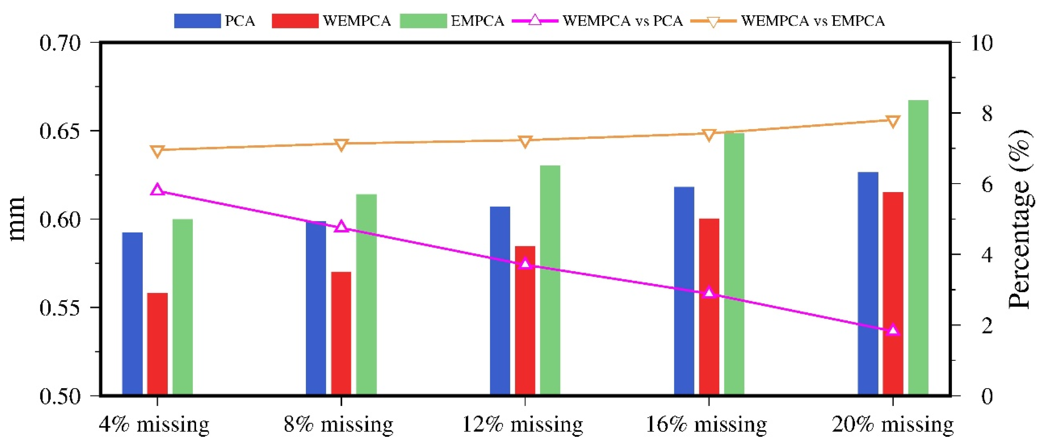
3.1. Simulation Experiments and Analysis

Simulation experiments are designed first to evaluate the performance of WEMPCA method in extracting CME from GNSS position time with both missing elements and noise. For this purpose, we initially randomly picked 14 stations from the GNSS network of Xinjiang province and then used the classic PCA approach to extract the CME of these selected stations as the true signal (CME_true). Moreover, we used the Hector software [42] to generate noise ε based on the formal errors of associated GNSS stations. The noise models “White + GGM (Generalised Gauss Markov)” were employed in the simulation processing, with the fraction of white noise $\varphi =0.35$ and spectral index $\phi =0.6$, respectively. Finally, the simulated dataset matrix $X_{\mathrm{sim}}$ was constructed by $X_{\mathrm{sim}}=CM{E}_{\mathrm{true}}+\mathsf{\epsilon }$. For quantitative comparison of WEMPCA, EMPCA, and PCA methods, we repeated the same experiment 100 times, with different simulated datasets $X_{\mathrm{sim}}$ but the same initialization scheme.

To evaluate the influence of noise amplitude on CME extraction, we scaled the formal error from 0.2 to 1.0 with 0.2 increments to generate the noise ε, and no missing data was introduced into the dataset $X_{\mathrm{sim}}$ in this simulation experiment.

Table 1. The RMS of difference between extracted CME and true CME in the North component under varying scaled formal errors using WEMPCA, EMPCA and PCA filtering methods.

Scaled	WEMPCA			EMPCA			PCA			Improvement (WEMPC Relative to PCA)
	Max	Min	Mean	Max	Min	Mean	Max	Min	Mean
0.2	0.19	0.18	0.18	0.20	0.19	0.19	0.20	0.19	0.19
0.4	0.38	0.35	0.36	0.41	0.38	0.39	0.41	0.38	0.39
0.6	0.56	0.53	0.55	0.61	0.57	0.59	0.61	0.57	0.59
0.8	0.75	0.71	0.73	0.85	0.76	0.81	0.85	0.76	0.81
1.0	0.93	0.88	0.91	1.09	1.00	1.05	1.09	1.00	1.05

shows the RMS of the difference between extracted CME (CME_extract) and real CME_true (hereinafter referred to as RMS_diff) for the North component under varying scaled formal errors using different filtering methods. It reveals that the RMS_diff values of these three methods become larger with increasing magnitude of formal errors, and WEMPCA outperforms the other two approaches, namely EMPCA and PCA, during all the 100 simulation experiments. The mean relative improvements of WEMPCA over EMPCA and PCA are 5.20%, 6.13%, 7.39%, 9.68%, and 12.89%, respectively, under formal error scaled from 0.2 to 1.0 with 0.2 increments. Notably, the results of EMPCA and PCA are identical since no missing values were introduced into the dataset $X_{\mathrm{sim}}$. Similar results can be obtained for the East and Up components. Thus, we may conclude that the magnitude of noise can significantly affect CME extraction, and that the WEMPCA method can be used to remove CME from noisy GNSS position time series with high accuracy.

To illustrate the impact of missing data on the precision of CME recognition, Figure 3 shows the RMS_diff of the North component with varying percentages of missing data using PCA, EMPCA, and WEMPCA methods. It should be noted that in each of the 100 simulation experiments, no noise ε is added, and elements are cut off from CME_true at 4% to 20% with 4% increments to simulate the missing data. In this case, WEMPCA and EMPCA have the same weight matrix $W$, and there will be no difference between WEMPCA and EMPCA at this point.

From Figure 3, we can see that the WEMPCA/EMPCA methods are much more robust to missing data, and the extracted results are closer to the original CME. The results of PCA method rise considerably with the increasing amount of missing data, whereas the WEMPCA/EMPCA algorithm results change very little, even when 20% of the observations are deleted from the time series. Therefore, we conclude that the WEMPCA/EMPCA method is effective at extracting CME with minimizing the impact of missing data.

Finally, to explicitly show the performance improvement of WEMPCA in extracting CME from GNSS position time series that contain both missing values and noise, we take the simulated $X_{\mathrm{sim}}$ corresponding to 0.6 scaled factor in Table 1 as the initial dataset and then pick up 4% to 20% with 4% increments elements as missing data by assigning them a constant value of 9999.0 to crosscheck the WEMPCA algorithm. Figure 4 shows the results of RMS_diff and the relative improvement percentage of applying WEMPCA, EMPCA, and PCA to the simulated $X_{\mathrm{sim}}$ of the North component. As we can see, the RMS_diff values of all three methods rise with increasing missing data, and the WEMPCA algorithm always has outstanding performance over the other two methods. With a data deletion rate ranging from 4% to 20%, the relative improvements of WEMPCA over PCA and EMPCA ranged from 5.80% to 1.83%, 6.96% to 7.81%, respectively. As a result, it is critical to account for formal errors while filtering GNSS position time series, and our approach is to confirm this to be an effective alternative way to obtain CME from noisy and missing GNSS position time series.

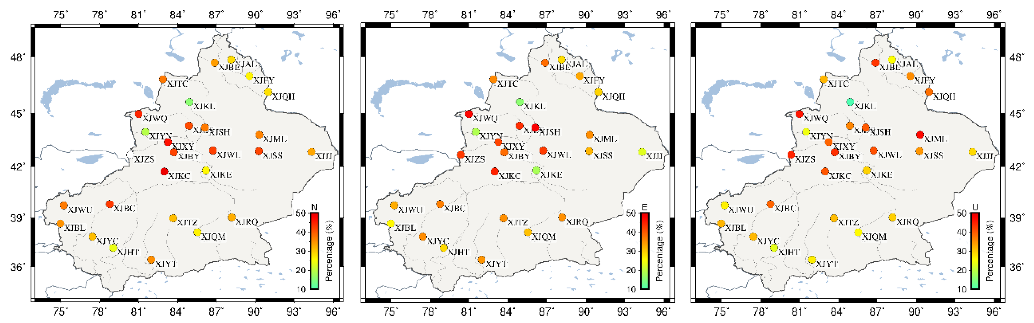
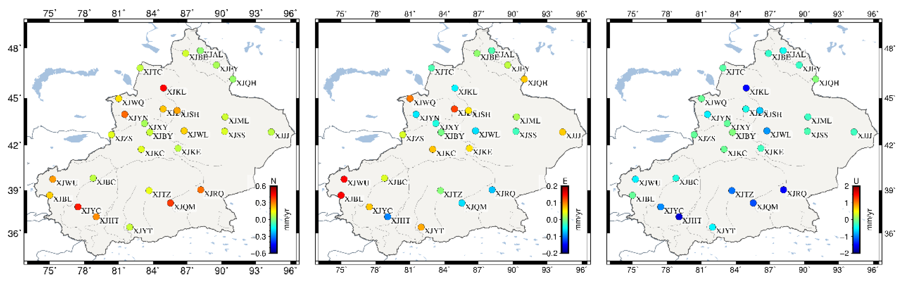
3.2. WEMPCA Filtering of Real GNSS Position Time Series

Figure 5 shows the first three scaled PCs (top panels) and their corresponding spatial responses (bottom panels) in the North, East, and Up directions for the 28 Xinjiang GNSS stations obtained using the WEMPCA approach. To make the comparison more intuitive, we slightly modify the quantitative criteria defined in Dong et al. [21] by scaling all the eigenvectors using the maximum absolute value of the first eigenvector. We can see that only the first scaled eigenvectors have the same sign and exhibit a significant positive spatial response with between-station differences for all three components. The mean spatial responses are 70.11%, 66.53, and 52.45% for the NEU component, respectively, whereas the minimum spatial responses are 43.24% for the North (XJJJ), 35.77% for the East (XJJJ), and 34.99% for the Up (XJKL).

The second and third PCs, on the other hand, have entirely distinct properties. Both show the uneven geographical distribution and oscillate interactively in spatial patterns. Additionally, for the second and third PCs, some stations, such as station XJYN in the North and Up components and station XJBL in the East component, exhibit significantly larger spatial responses than the other stations, suggesting that they reflect mostly local effects. Hence, we will only use the first PC and its corresponding eigenvectors to reconstruct CME for the following analysis.

3.3. Analysis of CME Time Series

Figure 6 presents the average CME (right panels) of the 28 GNSS stations in the North, East, and Up components, as well as the associated Lomb Scargle power spectral density (left panels). It reveals that the amplitude of CME in the Up direction is larger than that in the North and East. The standard deviation of CME is 1.28 mm, 1.22 mm, and 4.08 mm for the North, East, and Up components, respectively. In addition, the draconitic signal [43], which has frequencies of 1.04 cycle per year (cpy) and its higher harmonics, shows significant peaks in all three CME Lomb Scargle power spectral density, and we illustrated the first eight draconitic harmonics using brown-dash lines in the right panel of Figure 6. These signals are thought to be primarily related to the GPS constellation’s repetition periods in inertial space with regard to the Sun. Thus, we can conclude that the draconitic signal also played a part in regional CME. Furthermore, the slopes of CME spectra in the N and U components are close to −1, implying that the CME noise characteristics in these directions are proximate to flicker noise. However, the slopes of CME in the E direction show slightly different characteristics, with flicker noise presenting at low frequencies and white noise emerging at high frequencies.

The noise characteristic of the average CME time series was then analyzed using the Hector software. The result shows that the fractions of flicker and white noise in the average CME are 0.54, 0.76, 1.0 and 0.46, 0.24, 0.00 for North, East, and Up, respectively. Hence, we deduce that CME primarily involves flicker noise, with white noises present in some directions.

3.4. CME Impact on the GNSS Position Time Series

Figure 7 illustrates the canonical correlation coefficients of the 28 GNSS residual time series, as well as their corresponding histograms, before and after filtering the CME. Here, we utilized the Canonical Correlation Analysis [44] (CCA) instead of traditional Pearson’s correlation to calculate the correlation coefficients of two GNSS stations. CCA is a multivariate statistical technique that allows us to identify and explore the relationship among multidimensional variables. It can be used to model correlations between two multivariate datasets by finding linear combinations of variables that maximally correlate. Since the CME are regionally correlated, it is more appropriate to evaluate the influence of CME by examining the overall correlation changes in all three directions rather than individual changes. Our CCA result indicates that the interstation correlations for unfiltered residual time series exhibit strong associations among the 28 GNSS stations, with an average value of 0.64 and a maximum correlation of 0.88 between station XJKC and XJZS (about 240 km apart).

In addition, histograms of unfiltered residual time series reveal that the correlation coefficients vary between 0.40 and 0.90, with most values (about 77.25%) centered around 0.55~0.70. These findings confirm that there do exist significant spatial correlation errors in the regional GNSS network, which must be removed before scientific research and application. After filtering the CME by WEMPCA, the canonical correlation coefficients were significantly reduced to 0.29, representing an average reduction of 54.7%. Its histograms similarly reveal a significant drop, with majority values (79.90%) clustering around 0.15~0.35. Therefore, we conclude that our approach can efficiently reconstruct CME and decrease the spatial correlation error for the regional GNSS network.

Figure 8 reveals the RMS reduction ratios of NEU directions after removing CME from the 28 GNSS residual time series. It can be noticed that the RMS clearly decreases for all three components after filtering CME, with average decline ratios of 34.88%, 34.09%, and 33.73% for the NEU components, respectively. The maximal RMS reduction ratios are 50.58% at station XJZS for the North component, 48.29% at station XJSH for the East, and 47.08% at station XJML for the Up component. By comparison, the minimal RMS reduction ratios are 15.56%, 15.62% and 9.10% at station XJKL for all three components. Particularly, GNSS stations (e.g., XJSH, XJBY, and XJDS) in the Tien-Shan area exhibit greater RMS reduction than others, which is likely due to the remarkable hydrological changes [45] in this region.

Table 2. Standard deviations of PLN and WN amplitudes for the 28 GNSS position time series in NEU directions before and after filtering CME with WEMPCA.

No.	Station	N				E				U
		Unfiltered		Filtered		Unfiltered		Filtered		Unfiltered		Filtered
		PLN	WN	PLN	WN	PLN	WN	PLN	WN	PLN	WN	PLN	WN
1	XJAL	6.25	0.65	4.60	0.53	4.53	0.68	3.05	0.50	20.80	0.12	17.03	1.57
2	XJBC	5.17	0.66	2.29	0.58	4.84	0.95	2.46	0.78	14.39	2.14	7.69	2.10
3	XJBE	5.30	0.76	2.79	0.63	4.32	0.65	2.34	0.57	15.89	0.07	8.01	1.50
4	XJBL	6.47	0.68	3.22	0.66	6.18	1.15	4.06	0.92	16.25	2.27	9.33	1.89
5	XJBY	4.69	0.63	2.22	0.57	4.04	0.74	2.07	0.62	12.72	2.03	5.32	1.94
6	XJDS	5.09	0.63	2.00	0.59	3.91	0.74	1.53	0.59	12.89	0.02	5.47	1.78
7	XJFY	4.33	0.64	2.54	0.59	3.63	0.57	2.22	0.56	13.07	0.01	7.35	1.78
8	XJHT	5.07	0.61	3.01	0.59	4.58	0.86	2.86	0.69	12.43	2.04	8.08	1.82
9	XJJJ	2.88	0.48	2.84	0.42	2.42	0.55	2.39	0.55	9.17	1.33	6.65	1.97
10	XJKC	4.51	0.54	1.60	0.49	3.82	0.70	1.44	0.58	12.96	1.65	5.96	1.97
11	XJKE	4.44	0.64	2.70	0.63	3.90	0.80	2.53	0.66	12.81	2.05	6.52	2.43
12	XJKL	6.71	0.89	4.68	0.80	5.58	0.87	4.15	0.67	18.41	2.79	13.95	3.08
13	XJML	4.17	0.54	2.35	0.47	3.13	0.56	2.03	0.39	11.64	0.26	5.48	1.45
14	XJQH	4.26	0.65	2.70	0.58	3.58	0.33	2.15	0.16	13.07	0.02	6.38	1.32
15	XJQM	3.72	0.45	2.68	0.43	3.35	0.63	2.16	0.43	11.37	1.44	7.93	1.49
16	XJRQ	3.32	0.43	2.36	0.39	2.71	0.55	1.83	0.41	10.01	0.66	6.33	0.58
17	XJSH	4.92	0.63	2.32	0.53	3.71	0.69	1.37	0.48	13.46	1.28	5.63	1.93
18	XJSS	3.51	0.45	2.36	0.47	2.61	0.55	1.91	0.48	10.60	0.01	6.05	1.68
19	XJTC	5.49	0.75	2.27	0.67	4.95	0.99	2.48	0.91	15.65	1.70	8.48	2.16
20	XJTZ	4.14	0.54	2.35	0.47	3.67	0.73	1.92	0.57	11.63	1.67	7.11	1.53
21	XJWL	4.58	0.55	1.95	0.54	3.30	0.69	1.46	0.51	11.97	1.16	5.35	1.73
22	XJWQ	6.21	0.87	2.42	0.77	4.99	0.89	2.26	0.66	16.78	1.64	7.70	2.30
23	XJWU	6.68	0.88	3.21	0.75	6.92	1.21	4.66	0.97	19.18	2.96	12.19	2.67
24	XJXY	5.11	0.63	1.78	0.66	3.98	0.69	1.67	0.56	14.97	1.87	7.77	2.09
25	XJYC	5.56	0.63	2.84	0.56	5.69	0.96	3.31	0.71	17.53	2.56	10.99	2.25
26	XJYN	6.95	0.74	4.60	0.78	6.30	1.04	4.47	0.86	24.46	3.45	17.09	3.50
27	XJYT	4.53	0.54	2.55	0.34	4.28	0.78	2.42	0.48	13.59	1.68	8.94	1.34
28	XJZS	5.40	0.61	1.80	0.60	4.45	0.81	1.85	0.63	13.80	1.48	5.97	1.97
Mean		4.98	0.63	2.68	0.57	4.26	0.76	2.47	0.60	14.34	1.44	8.24	1.92

lists the standard deviations of PLN and WN amplitudes for the 28 GNSS position time series in NEU directions before and after filtering CME with WEMPCA. The average standard deviations of PLN and WN are presented in the last row of Table 2, and the maximum amplitude change values in each direction are separately marked in bold black. As we can see, the PLN amplitudes are significantly decreased after filtering CME in all three directions, with an average reduction ratio of 45.12%, 42.00%, and 43.41% for the North, East, and Up components, respectively. The maximum PLN amplitude reduction ratio can be found at station XJZS (66.76%) for the North component, station XJSH (63.17%) for the East, and station XJSH (58.20%) for the Up. However, the WN amplitude shows different features, which are reduced in the North and East components but enlarged in the up direction. Specifically, the average WN reduction ratios in horizontal directions are 9.19% (North) and 21.54% (East), while the vertical WN amplitude rises from 0.01 to 1.78 at station XJFY. This is because the white noise is most certainly caused by site-specific errors that CME filtering cannot eliminate.

Figure 9 shows the velocity differences (filtered minus unfiltered) between filtered and unfiltered time series of the 28 GNSS stations estimated by Hector software using PLN plus WN noise models. We find that the horizontal velocity differences are less than those in the vertical component, with the former average at 0.19 mm/year (North) and 0.03 mm/year (East), and the latter average at −0.56 mm/year (UP). The maximum differences are 0.85 mm/year at station XJKL for the North component, 0.21 mm/year at station XJWU for the East component, and −2.67 mm/year at station XJKL for the Up component. Overall, our results indicate that CME has a certain influence on the velocity estimation of GNSS stations and must be addressed appropriately.

Correspondingly, Figure 10 presents the velocity uncertainty in NEU directions before and after removing CME from the 28 GNSS stations by the WEMPCA method. Obvious uncertainty reductions can be noticed for majority stations, with average reductions of 43.51%, 38.64%, and 40.39 for the NEU components, respectively. The maximum reduction ratios for the North, East, UP directions are 74.87% at station XJKC, 72.90% at station XJSH, and 61.29% at station XJBE. Hence, we conclude that CME will inevitably affect the precision of GNSS position, velocity, and related uncertainties, and that our method is confirmed to be an effective method for filtering out CME.

4. Discussion

Spatial correlated errors, specifically CME, exist in regional GNSS networks and can have a significant effect on the precision of GNSS position, velocity, and associated uncertainties [31,32]. Thus, it is necessary to accurately filter out CME from the noisy and missing GNSS time series. Traditional filtering methods, such as stacking filtering, PCA, and ICA, can eliminate the impact of CME in the GNSS networks. However, as previously indicated, these algorithms have limitations. The WEMPCA algorithm described here provides a number of improvements over previous methods and outperforms them in several ways. A primary advantage of WEMPCA is that it can naturally incorporate weights on the input data, making the output eigenvectors less susceptible to measurement noise and more sensitive to true underlying signals [34]. Nevertheless, this weighting strategy may cause unexpected results when GNSS stations have strong local effects but with small formal errors [15]. Thus, the WEMPCA method is more appropriate for GNSS stations with weak local effects, and the GNSS stations with strong local effects must be identified and removed prior to CME extraction [24,33]. Moreover, compared with traditional PCA, the WEMPCA algorithm enables iterative extraction of only the first few PCs from noisy and missing GNSS time series, avoiding the need to keep the entire dataset at each step and therefore consuming less memory [34,38]. As a result, the WEMPCA is a robust and efficient alternative method for extracting CME from noisy and missing GNSS time series, particularly for large datasets.

5. Conclusions

In this research, the WEMPCA algorithm, which can properly incorporate measurement noise, was proposed to extract CME from the noisy and missing GNSS position time series. The simulation experiments reveal that the WEMPCA algorithm always outperforms the others, namely, traditional PCA and EMPCA. The relative improvements of WEMPCA over PCA and EMPCA are 1.83% and 7.81%, respectively, even when the simulated dataset $X_{\mathrm{sim}}$ contains 20% missing data and 0.6 scaled factor noise.

The WEMPCA method was then successfully used to process the 28 real noisy and missing GNSS position time series. Our results demonstrate that only the first PC exhibits significant positive spatial response, with average values of 70.11%, 66.53%, and 52.45% for North, East, and Up (NEU) components, respectively, indicating that they represent the CME. The analysis of CME also reveals that draconitic signal is definitely evident in lower harmonics, and CME predominantly consists of flicker noise with some white noise present in certain directions.

After removing CME, the canonical correlation coefficients significantly drop from 0.64 to 0.29, showing an average reduction ratio of 54.7%. The RMS values of residual time series are also obviously reduced for all three components, with an average decrease ratio of 34.88%, 34.09%, and 33.73% for the NEU components, respectively. In addition, the PLN and WN amplitudes exhibit distinct features after CME filtering, with the former declining significantly in all three directions, while the latter only falling in the North and East, but not in the Up component.

Meanwhile, the average velocity differences before and after filtering CME can reach 0.19 mm/year for the North, 0.03 mm/year for the East, and −0.56 mm/year for the Up, indicating that CME has a certain effect on GNSS station velocity estimation. After filtering the CME with WEMPCA, the velocity uncertainty can be decreased by 43.51%, 38.64%, and 40.39 on average for the NEU components, respectively. Therefore, we can conclude that the CME has an influence on the precision of GNSS position, velocity, and uncertainties, and that our strategy presents an effective method for mitigating the effects of CME.

References

1. Geng, J.; Pan, Y.; Li, X.; Guo, J.; Liu, J.; Chen, X.; Zhang, Y. Noise Characteristics of High-Rate Multi-GNSS for Subdaily Crustal Deformation Monitoring. J. Geophys. Res. Solid Earth 2018, 123, 1987–2002. [Google Scholar] [CrossRef]
2. Zheng, K.; Zhang, X.; Li, X.; Li, P.; Chang, X.; Sang, J.; Ge, M.; Schuh, H. Mitigation of Unmodeled Error to Improve the Accuracy of Multi-GNSS PPP for Crustal Deformation Monitoring. Remote Sens. 2019, 11, 2232. [Google Scholar] [CrossRef] [Green Version]
3. Geng, T.; Xie, X.; Fang, R.; Su, X.; Zhao, Q.; Liu, G.; Li, H.; Shi, C.; Liu, J. Real-time capture of seismic waves using high-rate multi-GNSS observations: Application to the 2015 Mw 7.8 Nepal earthquake. Geophys. Res. Lett. 2016, 43, 161–167. [Google Scholar] [CrossRef] [Green Version]
4. Caporali, A.; Floris, M.; Chen, X.; Nurce, B.; Bertocco, M.; Zurutuza, J. The November 2019 Seismic Sequence in Albania: Geodetic Constraints and Fault Interaction. Remote Sens. 2020, 12, 846. [Google Scholar] [CrossRef] [Green Version]
5. Guns, K.A.; Pollitz, F.F.; Lay, T.; Yue, H. Exploring GPS Observations of Postseismic Deformation Following the 2012 MW7.8 Haida Gwaii and 2013 MW7.5 Craig, Alaska Earthquakes: Implications for Viscoelastic Earth Structure. J. Geophys. Res. Solid Earth 2021, 126, e2021JB021891. [Google Scholar] [CrossRef]
6. Kang, Z.; Tapley, B.; Chen, J.; Ries, J.; Bettadpur, S. Geocenter motion time series derived from GRACE GPS and LAGEOS observations. J. Geod. 2019, 93, 1931–1942. [Google Scholar] [CrossRef]
7. Meindl, M.; Beutler, G.; Thaller, D.; Dach, R.; Jäggi, A. Geocenter coordinates estimated from GNSS data as viewed by perturbation theory. Adv. Space Res. 2013, 51, 1047–1064. [Google Scholar] [CrossRef]
8. Lavallée, D.A.; van Dam, T.; Blewitt, G.; Clarke, P.J. Geocenter motions from GPS: A unified observation model. J. Geophys. Res. Solid Earth 2006, 111, B05405. [Google Scholar] [CrossRef] [Green Version]
9. Thomas, I.D.; King, M.A.; Bentley, M.J.; Whitehouse, P.L.; Penna, N.T.; Williams, S.D.P.; Riva, R.E.M.; Lavallee, D.A.; Clarke, P.J.; King, E.C.; et al. Widespread low rates of Antarctic glacial isostatic adjustment revealed by GPS observations. Geophys. Res. Lett. 2011, 38, L22302. [Google Scholar] [CrossRef] [Green Version]
10. Simon, K.M.; Riva, R.E.M.; Vermeersen, L.L.A. Constraint of glacial isostatic adjustment in the North Sea with geological relative sea level and GNSS vertical land motion data. Geophys. J. Int. 2021, 227, 1168–1180. [Google Scholar] [CrossRef]
11. Yuan, P.; Jiang, W.; Wang, K.; Sneeuw, N. Effects of Spatiotemporal Filtering on the Periodic Signals and Noise in the GPS Position Time Series of the Crustal Movement Observation Network of China. Remote Sens. 2018, 10, 1472. [Google Scholar] [CrossRef] [Green Version]
12. He, X.; Montillet, J.-P.; Fernandes, R.; Bos, M.; Yu, K.; Hua, X.; Jiang, W. Review of current GPS methodologies for producing accurate time series and their error sources. J. Geodyn. 2017, 106, 12–29. [Google Scholar] [CrossRef]
13. Kreemer, C.; Blewitt, G. Robust estimation of spatially varying common-mode components in GPS time-series. J. Geod. 2021, 95, 13. [Google Scholar] [CrossRef]
14. Wdowinski, S.; Bock, Y.; Zhang, J.; Fang, P.; Genrich, J. Southern California permanent GPS geodetic array: Spatial filtering of daily positions for estimating coseismic and postseismic displacements induced by the 1992 Landers earthquake. J. Geophys. Res. Solid Earth 1997, 102, 18057–18070. [Google Scholar] [CrossRef]
15. Gruszczynski, M.; Klos, A.; Bogusz, J. A Filtering of Incomplete GNSS Position Time Series with Probabilistic Principal Component Analysis. Pure Appl. Geophys. 2018, 175, 1841–1867. [Google Scholar] [CrossRef]
16. He, X.; Bos, M.S.; Montillet, J.P.; Fernandes, R.M.S. Investigation of the noise properties at low frequencies in long GNSS time series. J. Geod. 2019, 93, 1271–1282. [Google Scholar] [CrossRef]
17. He, X.; Bos, M.S.; Montillet, J.-P.; Fernandes, R.; Melbourne, T.; Jiang, W.; Li, W. Spatial Variations of Stochastic Noise Properties in GPS Time Series. Remote Sens. 2021, 13, 4534. [Google Scholar] [CrossRef]
18. Nikolaidis, R. Observation of Geodetic and Seismic Deformation with the Global Positioning System; University of California: San Diego, CA, USA, 2002. [Google Scholar]
19. Tian, Y.; Shen, Z. Correlation weighted stacking filtering of common-mode component in GPS observation network. Acta Seismol. Sin 2011, 33, 198–208. [Google Scholar]
20. Márquez-Azúa, B.; DeMets, C. Crustal velocity field of Mexico from continuous GPS measurements, 1993 to June 2001: Implications for the neotectonics of Mexico. J. Geophys. Res. Solid Earth 2003, 108, 2450. [Google Scholar] [CrossRef]
21. Tian, Y.; Shen, Z.-K. Extracting the regional common-mode component of GPS station position time series from dense continuous network. J. Geophys. Res. Solid Earth 2016, 121, 1080–1096. [Google Scholar] [CrossRef]
22. Forootan, E. Statistical Signal Decomposition Techniques for Analyzing Time-Variable Satellite Gravimetry Data. Ph.D. Thesis, University of Bonn, Bonn, Germany, 2014. [Google Scholar]
23. Cheng, P.; Cheng, Y.; Wang, X.; Wu, S.; Xu, Y. Realization of an Optimal Dynamic Geodetic Reference Frame in China: Methodology and Applications. Engineering 2020, 6, 879–897. [Google Scholar] [CrossRef]
24. Dong, D.; Fang, P.; Bock, Y.; Webb, F.; Prawirodirdjo, L.; Kedar, S.; Jamason, P. Spatiotemporal filtering using principal component analysis and Karhunen-Loeve expansion approaches for regional GPS network analysis. J. Geophys. Res. Solid Earth 2006, 111, B03405. [Google Scholar] [CrossRef] [Green Version]
25. Ji, K.H.; Herring, T.A. Transient signal detection using GPS measurements: Transient inflation at Akutan volcano, Alaska, during early 2008. Geophys. Res. Lett. 2011, 38, L06307. [Google Scholar] [CrossRef]
26. He, X.; Hua, X.; Yu, K.; Xuan, W.; Lu, T.; Zhang, W.; Chen, X. Accuracy enhancement of GPS time series using principal component analysis and block spatial filtering. Adv. Space Res. 2015, 55, 1316–1327. [Google Scholar] [CrossRef]
27. Ma, X.; Liu, B.; Dai, W.; Kuang, C.; Xing, X. Potential Contributors to Common Mode Error in Array GPS Displacement Fields in Taiwan Island. Remote Sens. 2021, 13, 4221. [Google Scholar] [CrossRef]
28. Zhou, M.; Guo, J.; Shen, Y.; Kong, Q.; YUAN, J. Extraction of common mode errors of GNSS coordinate time series based on multi-channel singular spectrum analysis. Chin. J. Geophys. 2018, 61, 4383–4395. [Google Scholar] [CrossRef]
29. Ming, F.; Yang, Y.; Zeng, A.; Zhao, B. Spatiotemporal filtering for regional GPS network in China using independent component analysis. J. Geod. 2017, 91, 419–440. [Google Scholar] [CrossRef]
30. Li, W.; Li, F.; Zhang, S.; Lei, J.; Zhang, Q.; Yuan, L. Spatiotemporal Filtering and Noise Analysis for Regional GNSS Network in Antarctica Using Independent Component Analysis. Remote Sens. 2019, 11, 386. [Google Scholar] [CrossRef] [Green Version]
31. Shen, Y.; Li, W.; Xu, G.; Li, B. Spatiotemporal filtering of regional GNSS network’s position time series with missing data using principle component analysis. J. Geod. 2014, 88, 1–12. [Google Scholar] [CrossRef]
32. Li, W.; Jiang, W.; Li, Z.; Chen, H.; Chen, Q.; Wang, J.; Zhu, G. Extracting Common Mode Errors of Regional GNSS Position Time Series in the Presence of Missing Data by Variational Bayesian Principal Component Analysis. Sensors 2020, 20, 2298. [Google Scholar] [CrossRef] [Green Version]
33. Li, W.; Shen, Y. The Consideration of Formal Errors in Spatiotemporal Filtering Using Principal Component Analysis for Regional GNSS Position Time Series. Remote Sens. 2018, 10, 534. [Google Scholar] [CrossRef] [Green Version]
34. Bailey, S. Principal component analysis with noisy and/or missing data. Publ. Astron. Soc. Pac. 2012, 124, 1015. [Google Scholar] [CrossRef] [Green Version]
35. Bevis, M.; Brown, A. Trajectory models and reference frames for crustal motion geodesy. J. Geod. 2014, 88, 283–311. [Google Scholar] [CrossRef] [Green Version]
36. Jolliffe, I.T.; Cadima, J. Principal component analysis: A review and recent developments. Philos. Trans. R. Soc. A Math. Phys. Eng. Sci. 2016, 374, 20150202. [Google Scholar] [CrossRef] [PubMed]
37. Golub, G.H.; Van Loan, C.F.; Press, J.H.U.; Van Loan, P.C.F. Matrix Computations; Johns Hopkins University Press: Baltimore, MD, USA, 1989. [Google Scholar]
38. Roweis, S. EM algorithms for PCA and SPCA. Adv. Neural Inf. Processing Syst. 1998, 626–632. [Google Scholar]
39. Owari, T.; Kasahara, H.; Oikawa, N.; Fukuoka, S. Seasonal variation of global positioning system (GPS) accuracy within the Tokyo University Forest in Hokkaido. Bull. Tokyo Univ. 2009, 120, 19–28. [Google Scholar]
40. Bogusz, J.; Gruszczynski, M.; Figurski, M.; Klos, A. Spatio-temporal filtering for determination ofcommon mode error in regional GNSS networks. Open Geosci. 2015, 7, 140–148. [Google Scholar] [CrossRef] [Green Version]
41. Liu, N.; Dai, W.; Santerre, R.; Kuang, C. A MATLAB-based Kriged Kalman Filter software for interpolating missing data in GNSS coordinate time series. GPS Solut. 2017, 22, 25. [Google Scholar] [CrossRef]
42. Bos, M.; Fernandes, R.; Williams, S.; Bastos, L. Fast error analysis of continuous GNSS observations with missing data. J. Geod. 2013, 87, 351–360. [Google Scholar] [CrossRef] [Green Version]
43. Amiri-Simkooei, A. On the nature of GPS draconitic year periodic pattern in multivariate position time series. J. Geophys. Res. Solid Earth 2013, 118, 2500–2511. [Google Scholar] [CrossRef] [Green Version]
44. Hardoon, D.R.; Szedmak, S.; Shawe-Taylor, J. Canonical correlation analysis: An overview with application to learning methods. Neural Comput. 2004, 16, 2639–2664. [Google Scholar] [CrossRef] [PubMed] [Green Version]
45. Li, W.; Guo, J.; Chang, X.; Zhu, G.; Kong, Q. Terrestrial Water Storage Changes in the Tianshan Mountains of Xinjiang Measured by GRACE During 2003~2013. Geomat. Inf. Sci. Wuhan Univ. 2017, 42, 1021–1026. [Google Scholar] [CrossRef]
Figure 1. The geographical location and percentage of missing data for all 28 GNSS stations in Xinjiang province of China.
Remotesensing 14 01295 g001
Figure 2. Formal error of station XJKC in the North component.
Remotesensing 14 01295 g002
Figure 3. RMS of difference between extracted CME and real CME of North component with varying percentages of missing data by WEMPCA, EMPCA, and PCA filtering methods.
Remotesensing 14 01295 g003
Figure 4. RMS of difference between extracted CME and real CME of the North component with missing and noisy data by WEMPCA, EMPCA and PCA filtering methods.
Remotesensing 14 01295 g004
Figure 5. The first three scaled PCs and their associated spatial responses for the North (upper), East (middle), and Up (lower) components of the 28 Xinjiang GNSS stations computed using the WEMPCA approach.
Remotesensing 14 01295 g005aRemotesensing 14 01295 g005b
Figure 6. Average CME (left panels) in the North, East, and UP component for the 28 Xinjiang GNSS stations, as well as the associated Lomb Scargle power spectral density (right panels). Brown-dash lines indicate the draconitic oscillations (1.04 cpy) and their harmonics up to the 8th.
Remotesensing 14 01295 g006
Figure 7. Canonical correlation coefficients of the 28 GNSS residual time series, as well as their corresponding histograms, before and after filtering CME.
Remotesensing 14 01295 g007
Figure 8. RMS reduction ratios for the NEU component after removing CME from the 28 GNSS residual time series.
Remotesensing 14 01295 g008
Figure 9. Velocity differences between filtered and unfiltered time series for the North (left panel), East (middle panel), and Up (right panel) components of the 28 GNSS stations estimated by Hector software with PLN plus WN noise models.
Remotesensing 14 01295 g009
Figure 10. Velocity uncertainty for the NEU directions before and after removing CME from the 28 GNSS stations by WEMPCA method.
Remotesensing 14 01295 g010