Article

Multiple UAV Flights across the Growing Season Can Characterize Fine Scale Phenological Heterogeneity within and among Vegetation Functional Groups

1
U.S. Geological Survey Northern Rocky Mountain Science Center, Bozeman, MT 59715, USA
2
Department of Land Resources and Environmental Sciences, Montana State University, Bozeman, MT 59717, USA
3
Department of Biological Systems Engineering, University of Wisconsin-Madison, Madison, WI 53706, USA
*
Author to whom correspondence should be addressed.
Remote Sens. 2022, 14(5), 1290; https://doi.org/10.3390/rs14051290
Submission received: 25 January 2022 / Revised: 25 February 2022 / Accepted: 2 March 2022 / Published: 6 March 2022
(This article belongs to the Section Remote Sensing in Agriculture and Vegetation)

Abstract

:
Grasslands and shrublands exhibit pronounced spatial and temporal variability in structure and function with differences in phenology that can be difficult to observe. Unpiloted aerial vehicles (UAVs) can measure vegetation spectral patterns relatively cheaply and repeatably at fine spatial resolution. We tested the ability of UAVs to measure phenological variability within vegetation functional groups and to improve classification accuracy at two sites in Montana, U.S.A. We tested four flight frequencies during the growing season. Classification accuracy based on reference data increased by 5–10% between a single flight and scenarios including all conducted flights. Accuracy increased from 50.6% to 61.4% at the drier site, while at the more mesic/densely vegetated site, we found an increase of 59.0% to 64.4% between a single and multiple flights over the growing season. Peak green-up varied by 2–4 weeks within the scenes, and sparse vegetation classes had only a short detectable window of active phtosynthesis; therefore, a single flight could not capture all vegetation that was active across the growing season. The multi-temporal analyses identified differences in the seasonal timing of green-up and senescence within herbaceous and sagebrush classes. Multiple UAV measurements can identify the fine-scale phenological variability in complex mixed grass/shrub vegetation.

1. Introduction

Rangelands are widely distributed globally and contribute significant ecosystem services [1]. The grasslands, shrublands, and other ecosystems that make up rangelands are comprised of diverse plant species with divergent life-history strategies (e.g., annual vs. perennial), structural differences (e.g., grass vs. shrub), and photosynthetic pathways (e.g., C3 vs. C4), which creates pronounced spatial variability in plant function and high biodiversity [2,3,4]. Interannual variability in climate, coupled with community and abiotic differences, can lead to large interannual variability in rangeland vegetation function [5,6,7,8]. Due to the collective variability and complexity of vegetation communities, understanding of the drivers of rangeland vegetation processes (e.g., carbon accumulation, reproduction, productivity, nutrient availability, etc.) across scales is needed to develop effective management strategies and predictive models of changes in a dynamic world [9,10]. Ground-based measurements provide crucial information for understanding these processes but are limited in scope. Linking in situ measurements with remotely sensed data can expand the geographic extent of observation, furthering the ability to prioritize management efforts and aid in answering key ecological questions [11,12,13].
Data collected at high temporal frequencies and fine spatial extents may be necessary to detect complex patterns and ecologically relevant processes [14,15]. Multi-temporal analyses based on remote sensing are increasingly used to monitor ecosystems and their dynamics over multiple time steps and improve the thematic resolution of remote sensing products. For example, analyses of multiple remotely sensed images from within the same year are used to improve classification accuracy [16,17,18], measure species composition and coverage in shrublands [19], classify crop types [20], examine yields and performance [21,22], differentiate tree species in an urban environment [23], identify plants with C3 versus C4 photosynthetic pathways [24], detect invasive species [25], and examine the number of annual green-up cycles across ecosystems [26]. Importantly, examining continuous patterns can reveal new dynamics of a system across seasons and over multiple years [26,27,28].
Understanding the timing, magnitude, and duration of life-history events, phenology, forms a key aspect of the assessment of the function of vegetation communities [29]. Changes in phenology can lead to ecological disruptions, plant-herbivore mismatch, alterations to competitive interactions, and disrupted nutrient fluxes, e.g., [30,31,32,33]. Phenology and production of rangelands assessed at the community level has identified important spatial and temporal variability and trends [34,35,36,37]. However, differences in growing season length and timing exist among and within vegetation functional groups: aggregations of species with similar characteristics and ecosystem roles. Measuring heterogeneity at smaller spatial extents provides the ability to observe differences in species and functional groups such as temporal patterns in green-up, peak production, and senescence [38]. Measurement at the functional group level is needed for quantifying phenological mismatches, timing management and restoration actions, understanding the species-specific impacts of climate change, and connecting phenological processes between scales [32,38,39,40]. However, the spatial and temporal resolution needed to identify phenological events at smaller spatial scales, such as within species and functional groups, precludes many satellite-based remote sensing approaches [41,42]. In situ approaches can be time-consuming and logistically difficult across large spatial areas, which compromises our ability to observe ecosystem dynamics at all relevant scales in space and time [29].
The use of an unpiloted aerial vehicle (UAV) can examine such questions at appropriate spatial resolutions, link to aerial- and satellite-based systems [23,43,44,45], and build upon ground-based surveys [46,47,48,49]. Multi-flight UAV approaches can measure seasonal changes, e.g., [22,50,51], variability between individual plants and/or species [52,53], and can increase accuracy of classifications [54]. However, UAV approaches are not a panacea; there are multiple challenges and questions about approaches to be resolved. Phenology can be difficult to measure in dryland systems [55]. The sensors on UAVs, normally utilizing visible color and near-infrared (NIR) bands, work best for classifying dominant species, whereas rare species and some herbaceous species can be hard to identify [44], requiring additional specific data collection [51]. While using multi-temporal images can improve classification, matching scenes between UAV flights can be challenging, e.g., [42]. Furthermore, flight times and sensor payloads are limited on lightweight UAVs [43,56], constraining the size of sampling areas. Aerial systems (planes and helicopters) are used to map large extents of vegetation at fine spatial scales [45,57,58], measure canopy structure [59,60,61], and survey for wildlife [62]. While aerial platforms can carry larger payloads for longer time periods, they are more limited in takeoff and landing locations and come with increased costs [56]. Appropriate application of UAVs should consider survey area, the need for repeat flights, and research questions [43]. For example, UAVs are demonstrated to be particularly well suited to sampling ecosystem indicators in rangeland settings, e.g., [44,46,51].
Understanding phenology implies measuring vegetation at multiple intervals, which of course, incurs a cost. It is important to understand what inference can be gained (or lost) by measuring more (or fewer) times within a growing season. Due to onboard GPS accuracy limitations, approaches such as manual co-registration to known surface models [52], ground control points (GCPs) [22,51,63,64], photogrammetric image orientation [65,66], and identifying objects post-flight [42] are used to successfully align imagery from multiple UAV flights. Object-based and/or supervised image classification techniques demonstrate utility for high-resolution imagery, e.g., [54,67,68]. However, the lack of prior knowledge of classes within a scene can impact accuracy [69] and complicate classification decisions. Furthermore, some rangeland species (e.g., sagebrush, Artemisia tridentata) show intra-canopy variability from different growing season lengths for new versus prior season perennial leaves and semi-deciduous phenology [70,71]. However, while supervised classification techniques are often used for increased accuracy and a better understanding of classes, e.g., [72], unsupervised approaches identify spectral variation within a dataset [73] and may be better suited for detecting the phenological heterogeneity that exists among and within vegetation functional groups.
Therefore, a deeper investigation into the ability to use UAVs to identify within functional group phenological variability is a needed step in linking information across scales, approaches, and components of rangeland systems. Specifically, identification within-group phenological variability at fine spatial scales is a key component for monitoring and downscaling vegetation relationships to climate, providing scale-appropriate data on management, and studying ecological consequences of phenological change, e.g., [29,38,52]. The goal of this study is to examine tradeoffs in classification depth (e.g., identification of phenological differences) and accuracy between collecting data from individual versus multiple UAV flights during the growing season in rangelands. Multiple UAV flights were used to: (1) compare vegetation classification based on a single flight versus multiple flights, (2) examine the timing variations of green-up, peak productivity, and senescence within vegetation functional groups, (3) determine the increased information gained from various, multiple flight scenarios over a growing season, and (4) quantify the increased logistical and analytical effort of various flight scenarios. The prediction was that multiple flights over the growing season would increase classification accuracy due to detection of differences in phenology among vegetation functional groups and by accounting for spatial variability within functional groups, thus enabling better spectral differentiation of classes. In addition, accuracy improvement could be achieved with flights over the first half of the growing season, which would capture green-up variation and initial differences in senescence that would improve the differentiation of functional groups.

2. Materials and Methods
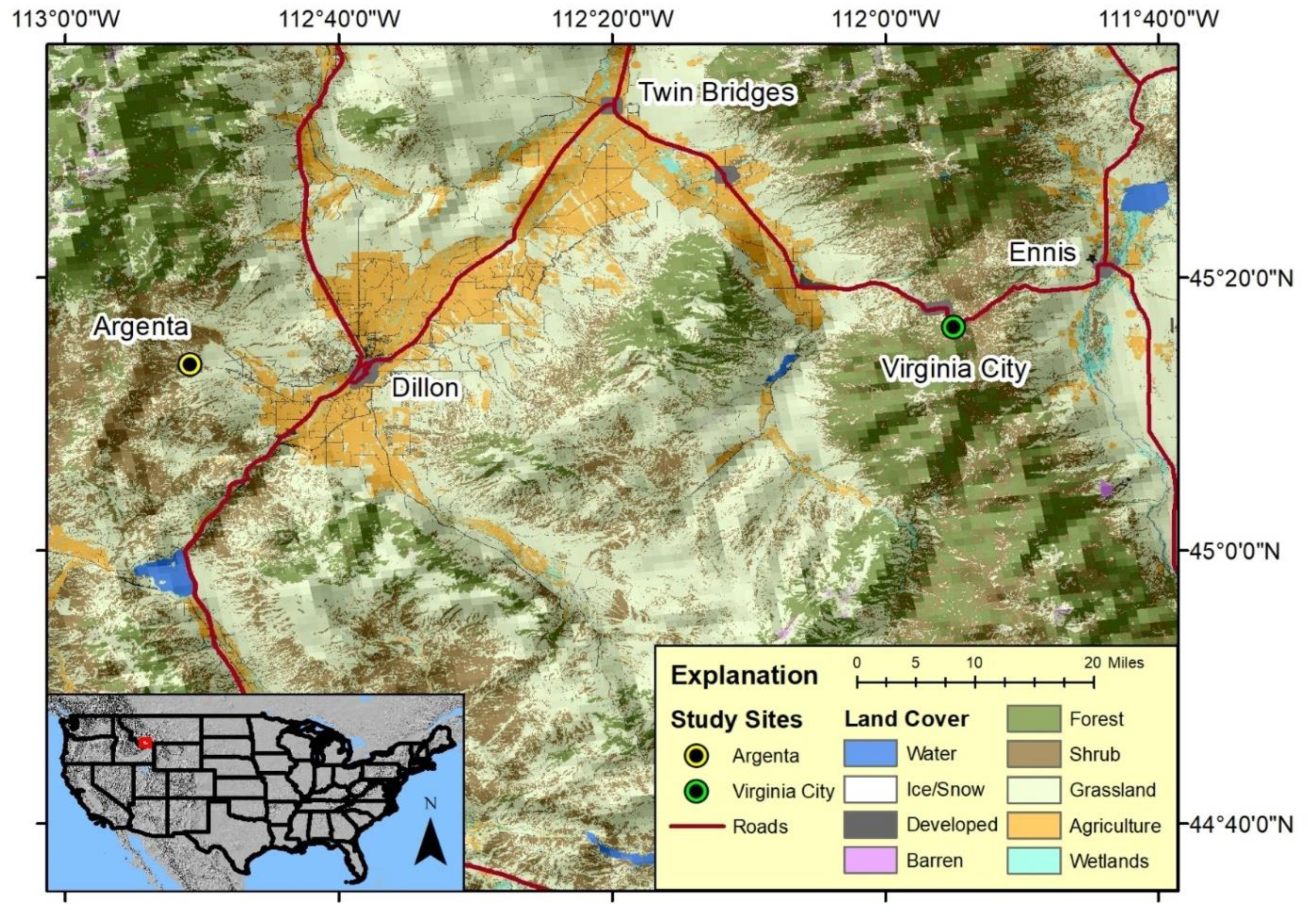
2.1. Study Areas

We selected two rangeland sites in southwestern Montana (Mont.), U.S.A., to capture two levels of precipitation of shrub-grassland sites in the region (Figure 1). Argenta, a drier and lower-elevation site, is located 20 km west of Dillon, Mont., in upland sagebrush steppe with primarily alluvial alfisols, sandy-loam soils, at approximately 1900 m elevation [74]. Mean monthly temperatures range from −7.3 to 16.4 °C with annual average precipitation of 283 mm (PRISM Climate Group, Oregon State University, http://prism.oregonstate.edu, created July 2012, accessed on 12 December 2019) [75]. The wetter, cooler, and higher elevation Virginia City site is located 5 km east of Virginia City, Mont., at an elevation of approximately 2240 m. Mean monthly temperatures range from −6.9 to 14.6 °C with annual average precipitation of 588 mm (PRISM Climate Group, Oregon State University, http://prism.oregonstate.edu, created July 2012, accessed on 12 December 2019) [75]. Soils are primarily mollisols with a mix of gravelly loam and stony loam on the steeper slopes [74]. Both sites are composed of sagebrush steppe; however, Virginia City generally has taller sagebrush, denser grasses, and less bare ground than Argenta.

2.2. Data Collection and Processing

We conducted numerous UAV flights (Table 1), each consisting of multiple missions per site (individual takeoff and landing to replace batteries, change camera settings, etc.), over the 2018 growing season from early May until October at each of the study sites. We flew a solo quadcopter (3DR, Berkeley, CA, USA) with a RedEdge-M (MicaSense, Seattle, WA, USA) multispectral camera, which captures five-band images (one band per lens corresponding to the following wavelengths, blue: 475 nm with 20 nm width, green: 560 nm with 20 nm width, red: 668 nm with 10 nm width, NIR: 840 nm with 40 nm width, and red edge 717 nm with 10 nm width). We programmed our UAV missions in Mission Planner (1.3.52, Ardupilot.org, accessed on 1 December 2021) to cover an approximately 300 × 300 m scene at each site. We recorded images of a calibrated reflectance panel (provided with the camera from MicaSense) before and after each mission to correct for illumination during processing. We conducted flights using a flight altitude of 43 m and airspeed of 5 m/s with the camera programmed to capture pictures every 2 s. This produced images with 65% forelap and sidelap and a roughly 3 cm ground sample distance (pixels). In addition, the RedEdge-M camera included an upward-facing light sensor that collected corresponding illumination data with each set of five-band images. We distributed GCPs at five marked locations across our scene to provide spatial referencing between flight dates.
At Argenta, we collected data over nine flights, covering the entire growing season (Table 1). Due to weather and snow cover, we were unable to collect early season data at Virginia City for flights 1 and 2 but were able to collect data for flights 3 through 9. However, a camera malfunction during flight 4 at Argenta and flight 7 at Virginia City resulted in missing data for portions of these scenes. Therefore, all multi-flight UAV classifications described hereafter are based on up to eight flights at Argenta and six at Virginia City (Table 1).
For each flight, we used MicaSense Python tools (https://github.com/micasense/imageprocessing, accessed on 1 December 2021) to convert images to aligned, corrected five-band stacks. This process included us using the calibration panel images to convert radiance values to reflectance values, correct for camera lens effects, and align each individual band together into a single image. We then inputted these images into Metashape (v1.5.2, Agisoft, St. Petersburg, Russia) for photogrammetric processing. Although the flights at each site followed the same flight plan, minor differences in extent and resolutions existed between the orthomosaics; therefore, we exported all orthomosaics for each site to the smallest extent and largest resolution identified across all flights to facilitate additional raster calculations. We transferred Metashape-produced products (e.g., orthomosaics, Digital Elevation Models (DEMs)) into ArcGIS 10.6 (ESRI, Redlands, CA) for additional processing steps as detailed below.
We employed a four-dimensional structure-from-motion approach (4D SfM) for our multi-date imagery [65,66] and used ground targets to assess the performance of image and flight alignment. The 4D SfM technique works by including survey photographs from all flights (i.e., dates) in the alignment, camera calibration, and georeferencing of ground control steps of the photogrammetry process. The process located objects (e.g., plants, rocks, litter, etc.) that remained in fixed locations through the entire time series. Effectively, 4D SfM identified thousands of ground control points that are consistent through the temporal period of the imagery to reference all photographs prior to building orthomosaics and other output products [65,66]. Following the 4D SfM alignment, we separated images by date and site to complete the remaining photogrammetry steps (generation of point cloud, surface models, orthomosaics, etc.). This process resulted in single five-band orthomosaics for each flight date: eight for Argenta and six for Virginia City. We calculated the normalized difference vegetation index (NDVI) for each UAV orthomosaic in ArcGIS using Image Analyst with associated red and NIR bands.
Active remote sensing sensors and structure-from-motion techniques utilized in aerial image processing produce three-dimensional models of the target scene, which allows for structural representations of vegetation [59,61,76]. The use of UAVs is expanding for mapping forest canopy structure, e.g., [60,76], and more recently, these techniques were applied to other vegetation types, e.g., [51,68,77,78]. In rangeland environments, shrub and grass structures may help in differentiating vegetation types [68]; therefore, we produced a canopy height model for our study sites. We estimated the vegetation height at each site from the UAV flight at the peak of the growing season (Table 1). We used the automatic Classify Ground Points function in Metashape, which classifies points within the dense point cloud as ground or other (i.e., vegetation) using three user-defined inputs. We explored multiple combinations of inputs (max angle, max distance, and cell size) to balance the ability of the classification algorithm to correctly assign the full canopy of shrubs while not missing a significant portion of ground points (e.g., being misclassified as vegetation). We created a digital surface model (DSM) from all points in the dense cloud and a digital terrain model (DTM), which uses only ground points and interpolates the elevation beneath vegetation. We calculated vegetation height using the raster calculator in ArcGIS by using the difference in DEMs technique, effectively subtracting the DTM from the DSM.
To provide additional information for classification, we created a texture raster layer based on the peak growing season flight for each site. We first created a single band image using the grayscale function from Image Analyst in ArcGIS. We equally weighted the red, green, and NIR bands from the peak growing season flight, effectively creating a grayscale version of a color infrared image. Then, using the focal statistics tool from Spatial Analyst, we calculated the standard deviation of a circular five-pixel region of the color infrared grayscale (single band) image. Window size and shape were chosen after testing other buffer distances for edge and scale effects [79,80]. Vegetation height and texture were normalized to match the range of NDVI values.

2.3. Image Classification

We classified vegetation for four sets of UAV flights (Table 1) to compare phenological information and classification accuracy differences between four scenarios of flight timing and frequency. These scenarios include (1) a single flight at the presumed peak of the growing season (hereafter “single”), (2) three flights over the growing season consisting of an early, peak, and end of season flight (hereafter “limited”), (3) flights during the early and core part of the growing season to cover initial green-up and the beginning of senescence (hereafter “spring”), and (4) using all available data covering the full growing season (hereafter “all flights”). We performed an iterative self-organized (ISO) unsupervised data analysis classification using NDVI from the selected flight(s) and vegetation height and texture data derived from the flight at the peak of the growing season. We allowed for a maximum of 30 classes. We repeated this approach for the multiple flight scenarios but included additional NDVI values with the same normalized vegetation height and texture. For Argenta, the all flights classification was based on 10 inputs (8 flights), the spring classification on 7 inputs (5 flights), and the limited classification on 5 inputs (3 flights). For Virginia City, the all flights classification was based on eight inputs (six flights), the spring classification on six inputs (four flights), and the limited classification on five inputs (three flights).
For each scenario, we examined the mean height and NDVI of the resulting classes along with visual interpretation to assign classes and collapsed classes together that could not be categorized into separate vegetation types, densities, or phenological patterns. For the single flight scenario, we used a single mean NDVI value; however, we used the mean NDVI values across included flight dates (i.e., a partial phenological curve) for each included flight for multiple flight scenarios. We first classified the image to identify a base set of six functional groups: bare ground, litter, sparse, medium, and dense herbaceous, and sagebrush. Differentiation between sparse, medium, and dense herbaceous categories was based on mean NDVI of the class (NDVI or peak NDVI for sparse between 0.2 and 0.3, medium between 0.3 and 0.4, and dense > 0.4), supplemented by visual inspection of pixels and areas of the class. Sagebrush classes also had an NDVI or peak NDVI of about 0.45, but vegetation height was higher (mean about 0.3 m versus < 0.1 m for herbaceous). Soil and litter classes were identified based on NDVI patterns that showed only minor deviations over the growing season (due to changes in moisture content and possible pixel mixing), height (for standing litter), and visual inspection of color and/or location in the scene. In addition, if possible for a given scenario, we identified subcategories of each of these classes to reflect differences in green-up and senescence timing and height.
We chose to use NDVI as our primary input into our classification algorithms as it is a surrogate for plant photosynthetic activity and was an indicator that matched our objective of examining phenological differences. In addition, even after post-processing, we had illumination differences due to clouds and shadows among flights which caused discontinuities on the five original bands produced by the MicaSense RedEdge-M camera that can impact the classification algorithms. Illumination differences were greatly reduced or eliminated by employing a ratio of bands such as NDVI, which removed brightness issues within and across flights.

2.4. Accuracy Assessment

To assess the accuracy of our classification scenarios, we performed analyst-based classification to derive reference data following recommendations for using the same orthomosaics as used for our classification, see [81,82]. At each study site, we created a stratified random sample of 1000 points, stratified on the classes derived from the all flights scenario. We used zonal statistics to calculate the mean NDVI for all flight classes for each flight date to create NDVI curves representing the phenological pattern for each class. Then, for each sample point, we extracted NDVI values at each flight date and vegetation height as derived from the peak growing season flight. Then, at each sample point, we deduced the reference classification for the point by comparing NDVI curves, height ranges, and RGB images from available flights. These reference data were then used to create a confusion matrix for each classification scenario at each site. Although reference data were based on all flight classifications (with subcategories), we collapsed subcategories into the main class to allow comparison across the full set of scenarios. In addition, we used our base set of six functional groups (bare ground, litter, sparse, medium, and dense herbaceous, and sagebrush) as a standard comparison of scenarios, as the single flight classification approach contains no subcategories. For all confusion matrices, we also calculated the kappa statistic (the classification agreement relative to random allocation) as a measure of accuracy [[73], but see [81] for limitations].

3. Results

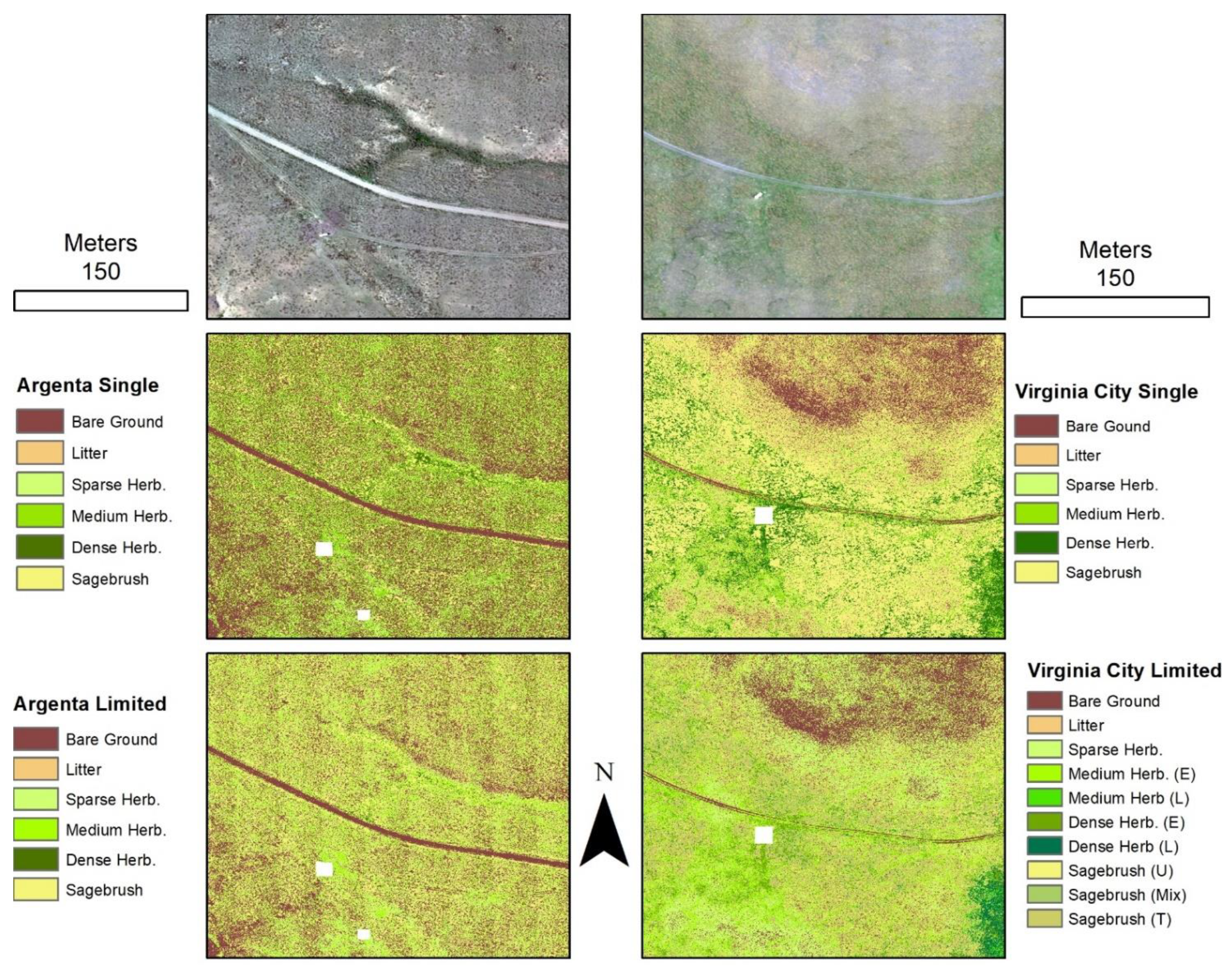
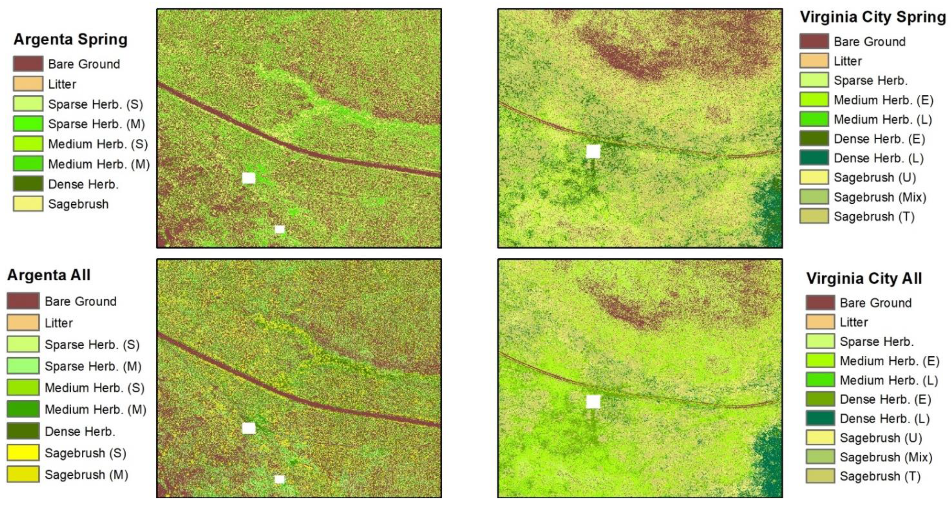
3.1. Flight Classifications

The single flight classifications based on the 12 June 2018, flight at Argenta and the 27 June 2018, flight at Virginia City resulted in our base set of six functional groups. Most multi-flight scenarios could identify different phenological patterns within functional groups, i.e., subcategories (Figure 2, see also Appendix A). Subcategories were defined in several ways because we found that areas within the same functional group were actively growing (or peaking) at different time periods. Subcategories were defined by differences in the length of the growing season (i.e., how long pixels had NDVI values above baseline), the timing of green-up (NDVI increase), peak values (day of peak NDVI), and senescence (when NDVI begins to quickly decline). Furthermore, at the Virginia City site, sagebrush heights covered a larger range, and we could differentiate sagebrush into two height classes that also coincided with the magnitude of NDVI values. Including subcategories, we differentiated 9 vegetation classes at Argenta (Figure 2, Figure 3 and Figure A1) and 10 classes at Virginia City (Figure 2, Figure 4 and Figure A2), using the all flights scenario for each site. In the sparse flights scenario, we were unable to identify subcategories at Argenta, which resulted in the 6 main classes (Figure A3); however, we identified the same 10 classes as in the all flight scenario at Virginia City (Figure A4). For the spring scenario, we could partially differentiate the 6 classes at Argenta, with differences observed in the herbaceous class but not in the sagebrush class (Figure A5), and fully differentiate all 10 classes at Virginia City (Figure A6).
Subcategories were identified within the herbaceous and sagebrush classes and represent different phenological responses within these functional groups (Figure 2, Figure 3 and Figure 4). At Argenta, NDVI slowly increased between flights 1 and 2, rapidly increased to a peak at flight 3, and then declined, with differences within herbaceous functional groups related to NDVI decline. The subclass ‘short season’ quickly declined after the peak at flight 3, whereas the moderate season remained close to peak values at flight 4, then declined quickly after flight 5. Flights 3 and 4 were 15 days apart, so these phenological differences represent at least two additional weeks of increased photosynthesis. Sagebrush short and moderate seasons were similar to herbaceous classes but shifted one additional week into the growing season (short season declines after flight 4, moderate after flight 5).
At Virginia City, senescence dates across classes were similar, and herbaceous subcategories were differentiated by early or late green-up dates. Early season herbaceous had a peak value at flight 3 (the first available at Virginia City) and slowly declined through flight 7, whereas late-season continued to increase through flights 4 and 5 before declining. Flights 3 and 5 were 37 days apart, representing a peak green-up value about a month later for the late-season phenological subcategories. Differences in sagebrush subcategories were related to height, with a short class (mean height about 0.1 m, primarily in the upslope portions of the scene) and a tall subcategory (mean height about 0.25 m). In addition, there was one class where pixels were mixed between sagebrush and herbaceous vegetation with an early peak green-up at flight 3 (from herbaceous vegetation) and a long season with plateaued NDVI values through flight 5 and a drop after, similar to sagebrush, and with height values (mean height of 0.24 m), similar to the tall class.

3.2. Accuracy, Class Differentiations, and Comparisons between Scenarios

To compare the four scenarios, we initially assessed the accuracy of each scenario in identifying the six base land cover classes (Table 2, Table A1, Table A2, Table A3, Table A4, Table A5, Table A6, Table A7 and Table A8). The accuracy from the single flight classifications at the Argenta site (50.6%) was marginally improved under the limited flights scenario (51.9%) and spring scenario (52.2%). However, the all flight scenario improved by almost 10% (61.4%). The accuracy of the all flight scenario, when including subcategories (the full nine identified including phenological differences), was similar to the single flight and other multiple flight scenarios (Table A9, overall accuracy = 51.8%). We were unable to identify any phenological differences (i.e., no subcategories) under the limited flights scenario. However, we were able to identify seasonal differences within the herbaceous categories with the spring scenario but with limited accuracy (45.6%).
At the Virginia City site, a similar class comparison (with six classes) resulted in an overall accuracy of 59.0% for the single flight scenario, 60.2% for the limited scenario, 61.6% for the spring scenario, and 64.4% for the all flight scenario (Table 2). When considering phenological differences, we were able to identify the same 10 classes in each of the multiple flight scenarios, but the overall accuracy of the limited (38.5%) and spring (40.0%) were poor compared to the all flight scenario (53.2%, Table A10).
Typically, the lowest class-specific accuracy rates at both sites were for the litter class across all scenarios (Table A1, Table A2, Table A3, Table A4, Table A5, Table A6, Table A7, Table A8, Table A9 and Table A10), with improvement in most situations between the single and multi-flight approaches (Table 2). The misclassification of litter was primarily with bare ground and sparse herbaceous classes. Herbaceous misclassification errors tended to be between densities (sparse, medium, and dense), in addition to some errors between dense herbaceous and sagebrush misclassifications at Argenta and to a lesser extent at Virginia City. The identification of phenological subcategories resulted in increased classification errors within the multi-flight classifications. These errors tended to be between the phenological classes (e.g., short versus moderate season length herbaceous); however, at Argenta, we also found classification errors between herbaceous and sagebrush classes. More flights (i.e., moving from single, to limited, to spring, to the all flights scenario) improved the classification of subcategories within functional groups (Table 2, Table A9 and Table A10).

4. Discussion

This study examined the ability of UAVs to identify fine-scale phenological heterogeneity, can be used to inform logistical decisions of future UAV studies (timing, number of flights, etc.), and illustrated options to effectively process data from multiple UAV flights. This approach successfully identified plant level phenological differences (i.e., differences in growing season length and timing within vegetation functional groups) and demonstrated improved classification accuracy by utilizing multi-flight UAV classification approaches. At both study locations, multi-flight scenarios improved vegetation classification accuracy over a single flight, mainly due to asynchronies in the timing and duration of herbaceous cover. Two main findings emerge from this study: (1) phenological heterogeneity at fine spatial scales can be identified by UAV flights, and (2) heterogeneity in phenological timing causes accuracy issues between class designations. The implications of these results include the ability to use these data to make finer scale ecological comparisons than satellite-based land surface phenology measures. In addition, while land surface phenology measures from satellite remote sensing can be influenced by the proportion of vegetation functional group, which may exhibit different phenological patterns, within a pixel [83], this study’s results suggest that within functional group heterogeneity needs to be considered as well. Furthermore, UAV-based studies provide phenological information at the plant or sub-plant level to compliment the broader spatial coverage available from satellite-based systems [22,42,52].

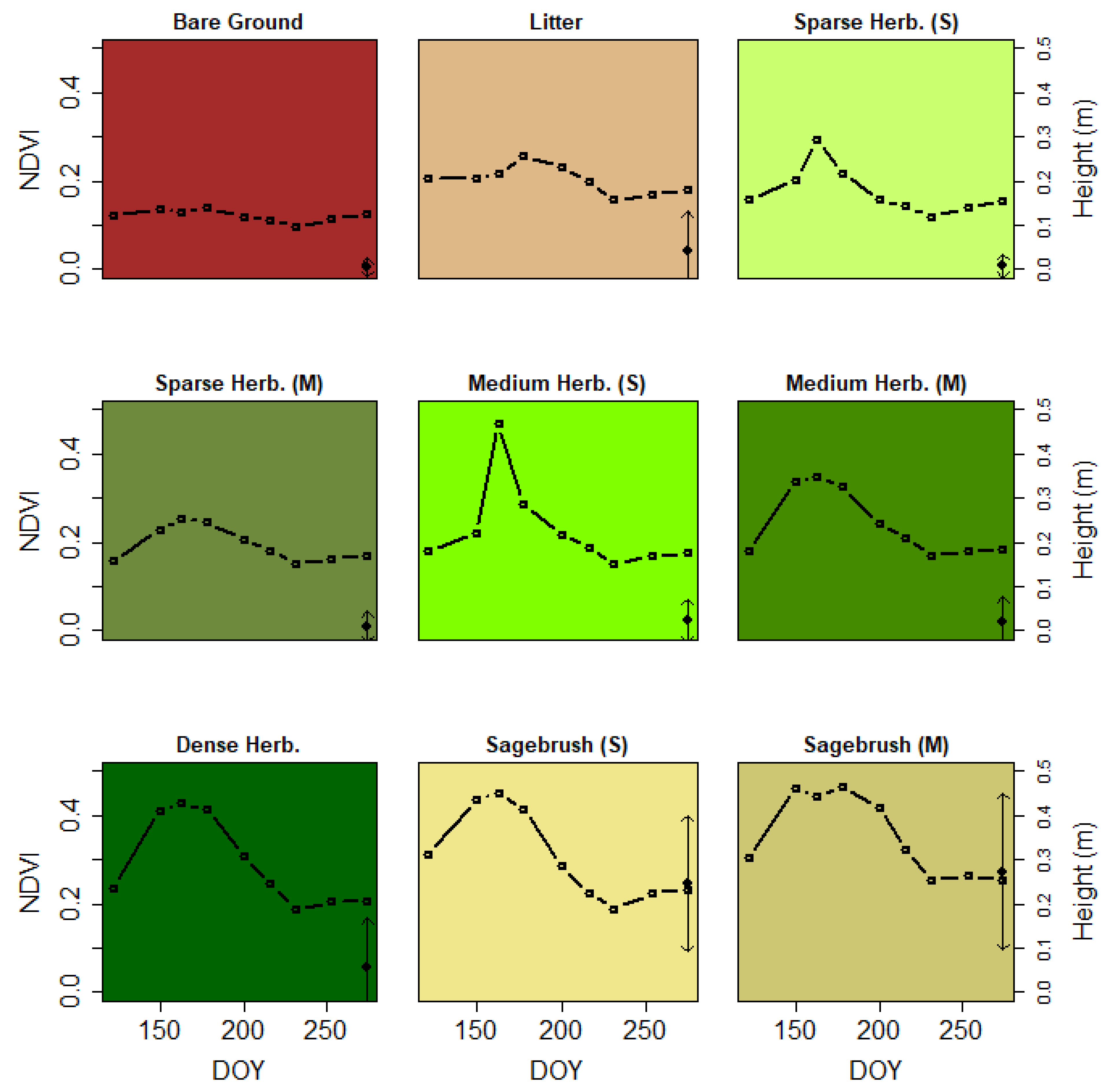
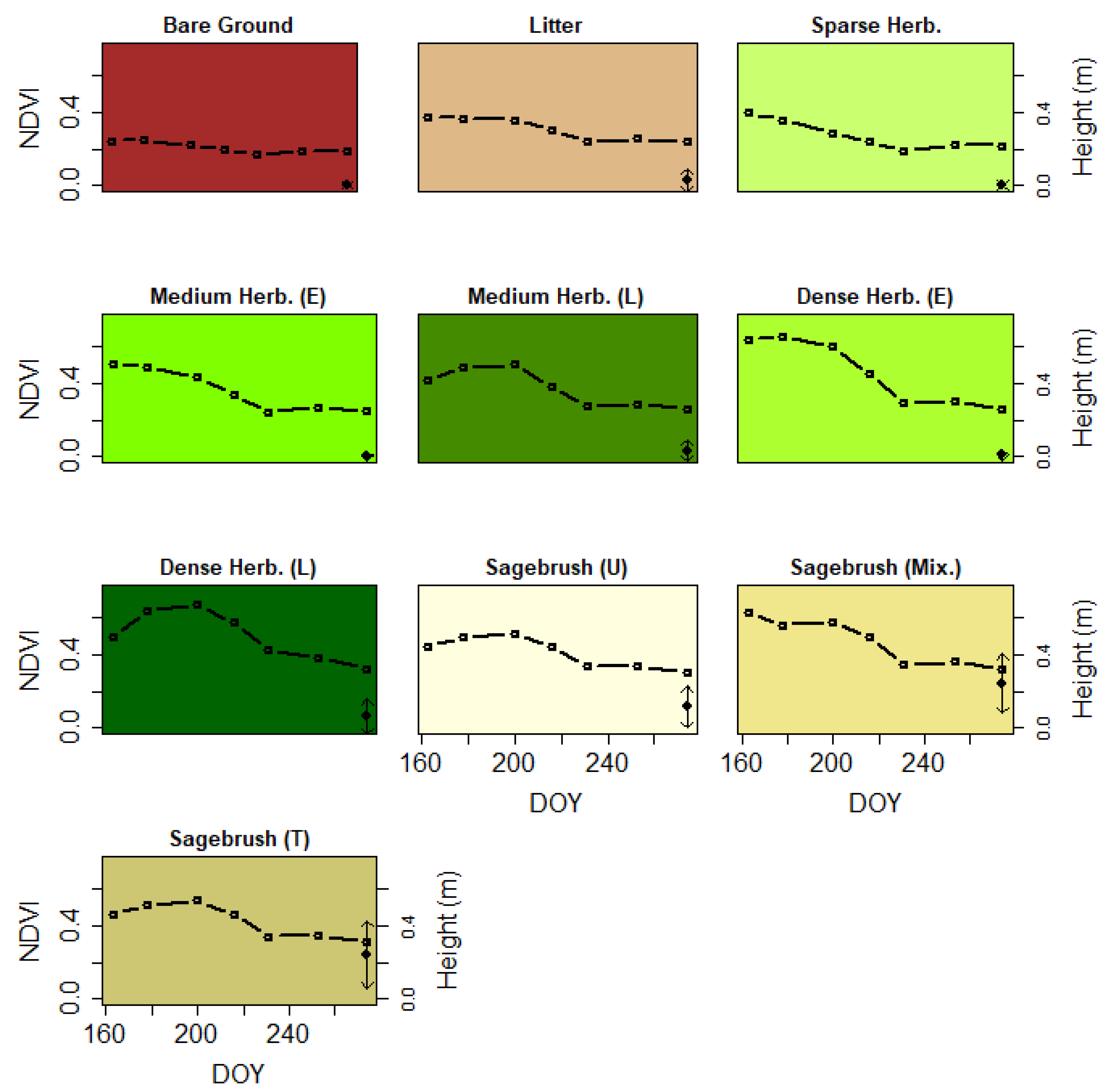
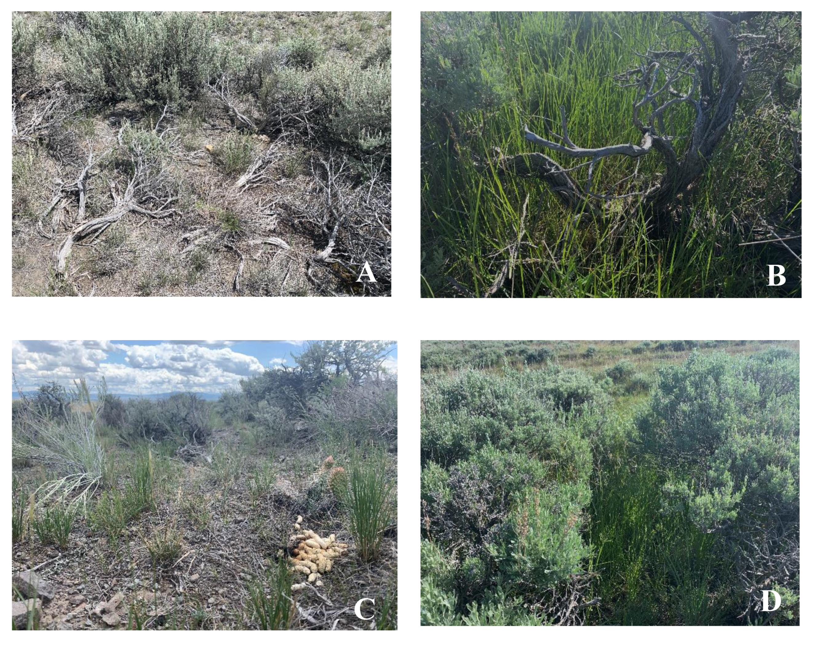
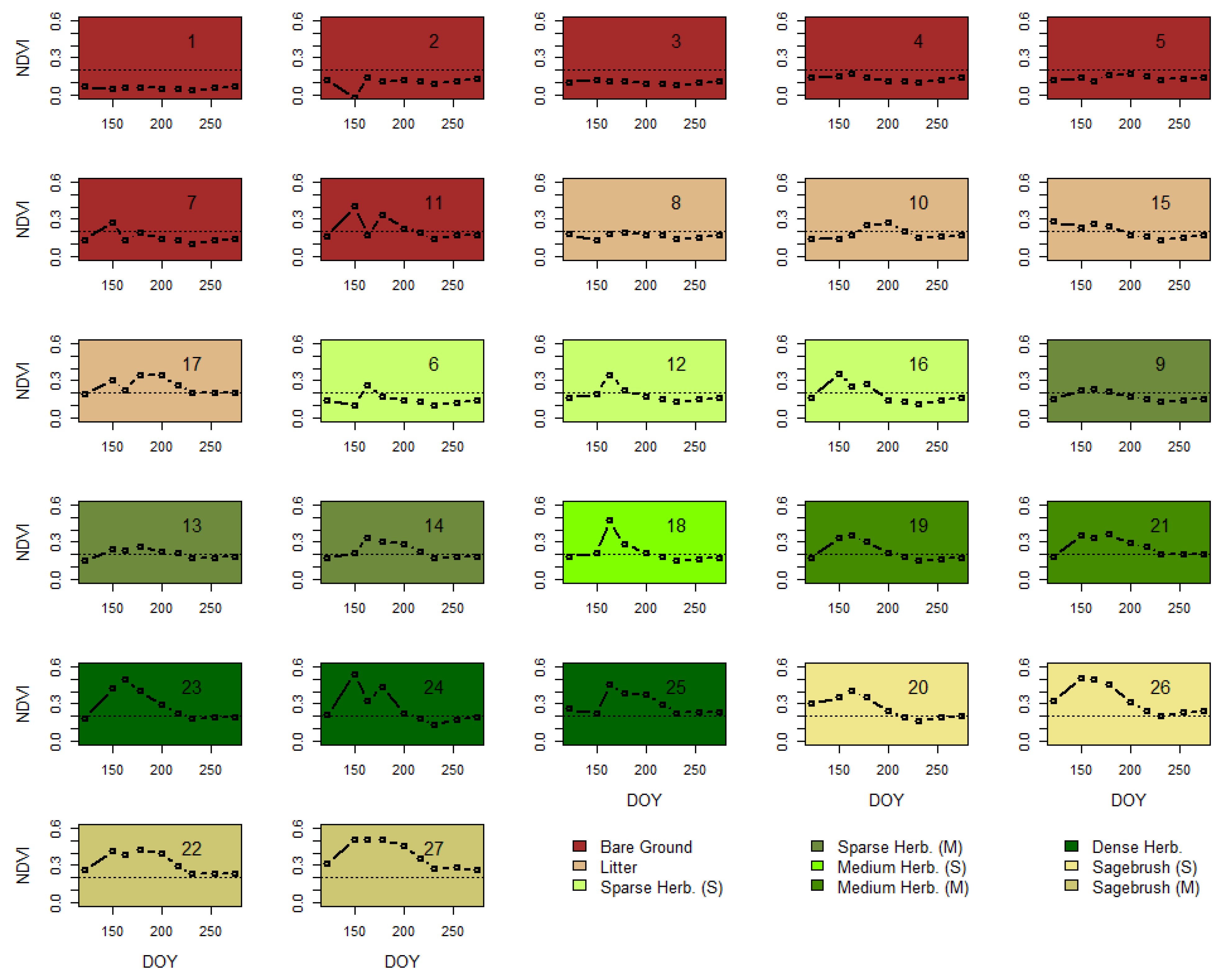
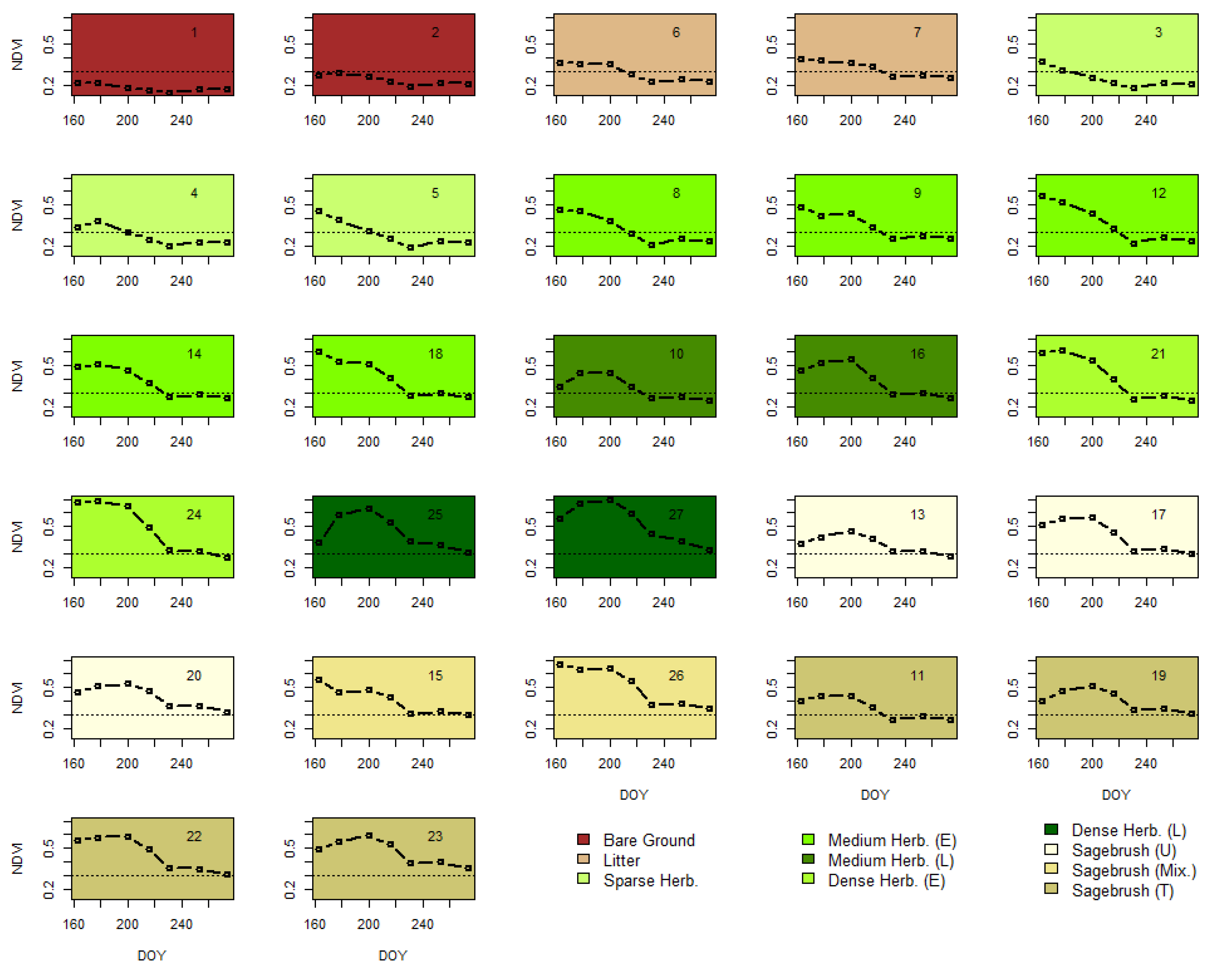
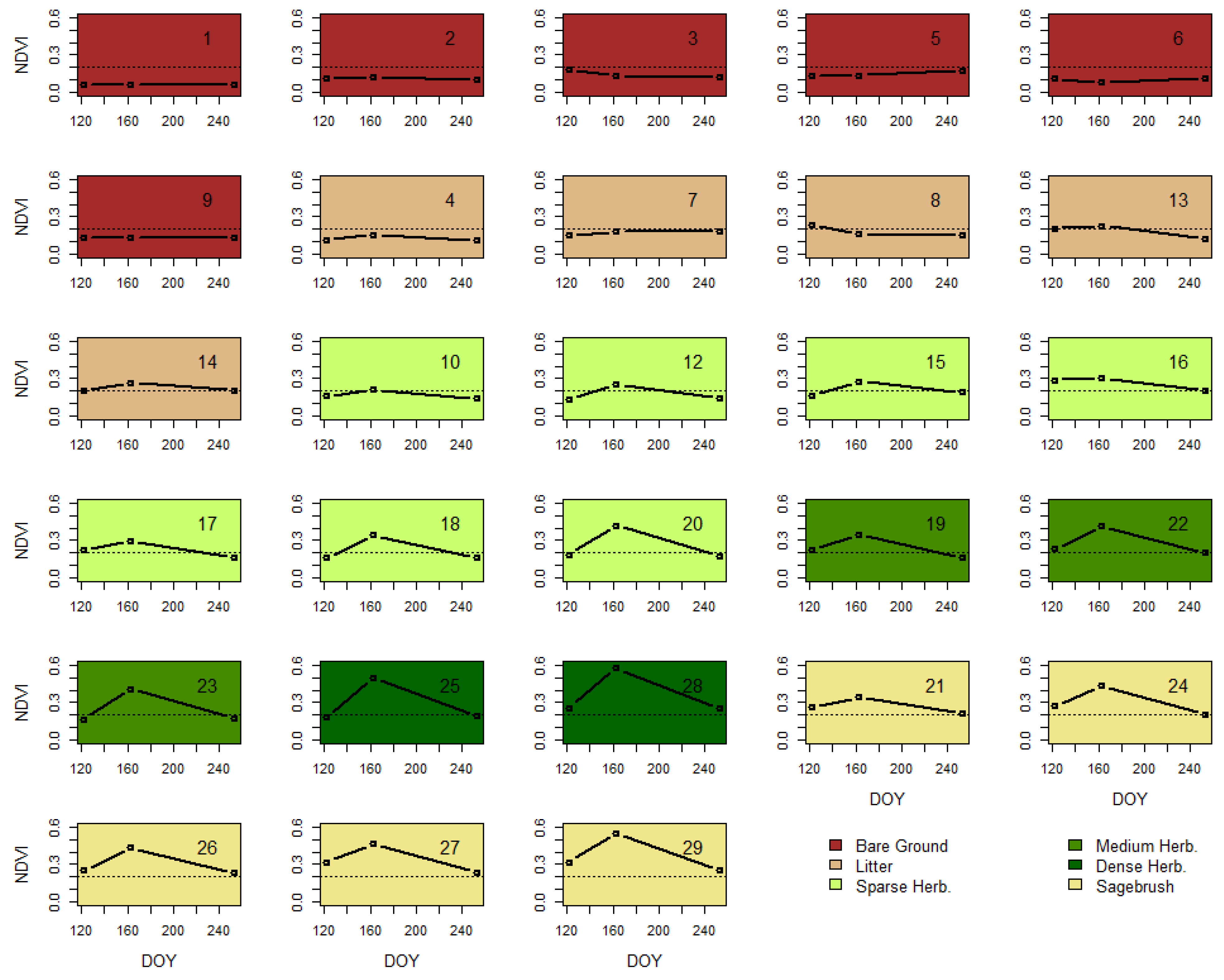
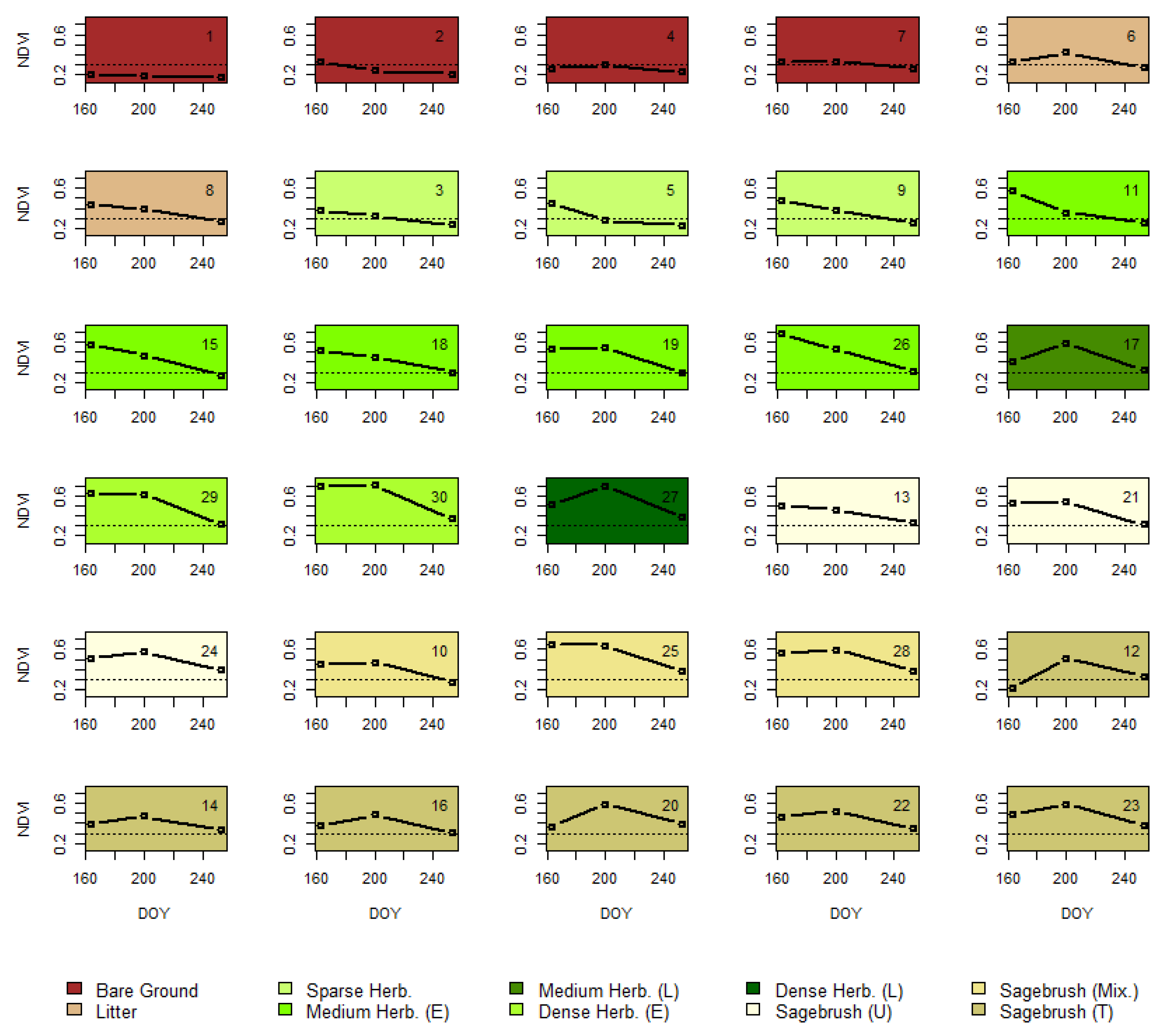
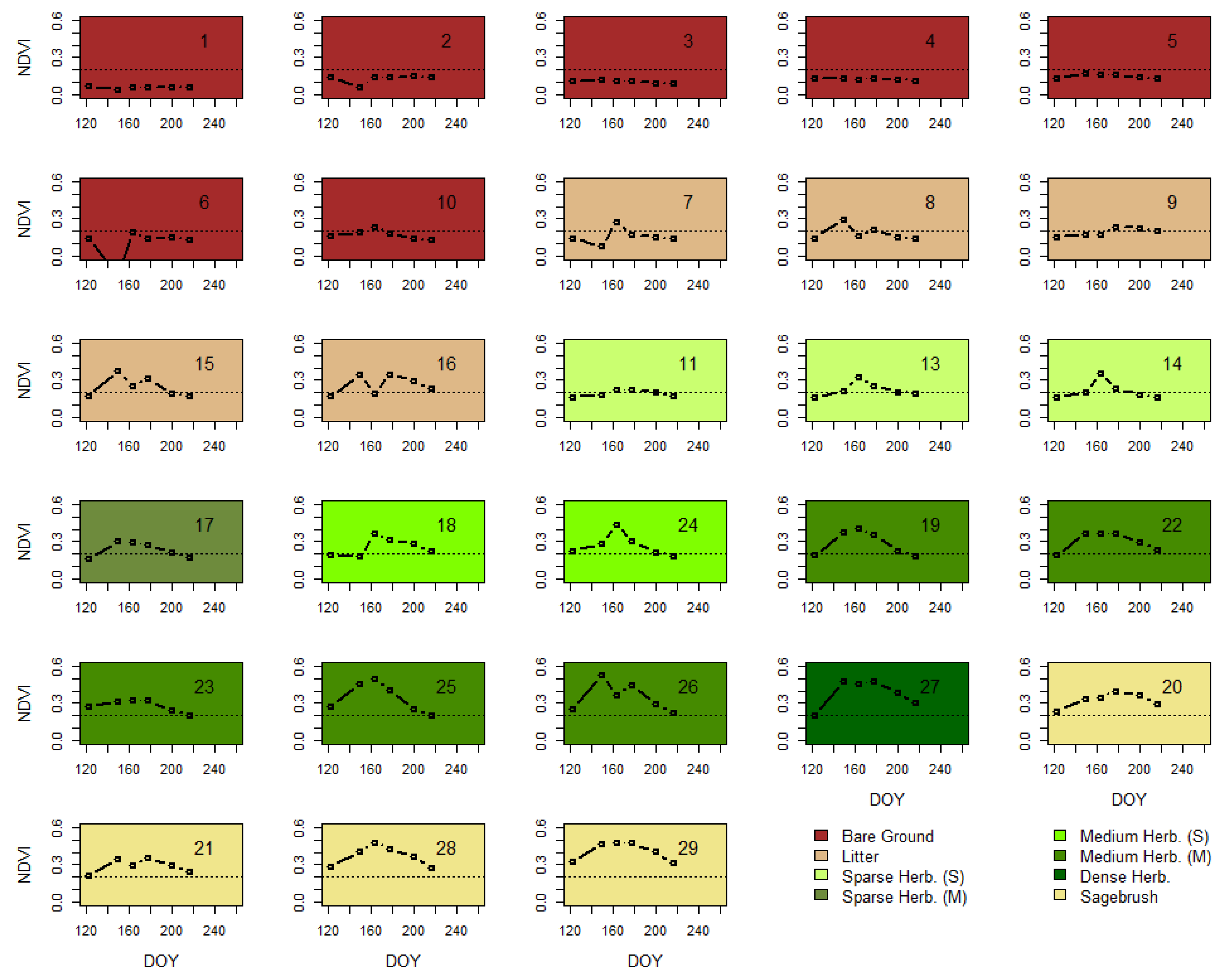
4.1. Phenological Heterogeneity within Functional Groups

Remote sensing is increasingly used to measure land surface phenology, which incorporates the mixed response of vegetation and background materials (e.g., soil and litter) within a sensor’s spatial resolution [83,84,85]. This study demonstrated the ability to examine patterns within functional groups at a fine resolution. Many of our multi-flight classification scenarios based on NDVI at multiple points during the growing season identified spatial variation within functional groups. These differences highlighted the role of topographic variations in phenology. For example, small valleys at Argenta have a longer growing season than upland locations, and there are seasonal asynchronies in herbaceous species between south-facing slopes and other areas at Virginia City. A study in marsh vegetation also found phenological differences in timing and duration within close spatial proximity, with implications for restoration and management [86]. Additional asynchronies in plant responses identified from remote sensing include differences in photosynthetic pathways [24], water use efficiency [28], growing conditions within fields [22], and variable intra- and inter-specific phenology [52]. Changing or variable vegetation phenology has consequences to other species and processes within the ecosystem [30,31,32,33,87]. Fine-scale measurement of variable vegetation functional group phenology is needed to inform restoration planning [86] and to better quantify the degree of phenological mismatch between members of an ecosystem under a changing climate. Understanding plant-level phenological differences as demonstrated here helps advance understanding of these processes.
At the drier Argenta site, there were functional group differences when plants were senescing and differences in the timing of green-up at the more mesic Virginia City site. These differences in limiting factors between sites may be difficult to identify a priori. In other sagebrush systems, communities in meadow (more mesic) locations had longer growing seasons compared to upland communities, with the difference due to earlier start of season dates [70]. In addition, new growth on sagebrush has a longer growing season [70], matching some of the sub-canopy variation identified herein, possibly also tied to the semi-deciduous pattern of sagebrush [71]. Phenology differences between and within species can be highly variable [23,52], asynchronies can be in the spring [70] or fall [42], and can be driven by variable growing conditions [22,70]. Building on phenology, temporal rangeland assessments can aid in ecological and land use studies. For example, high spatial resolution imagery can be used for within-season forage utilization [51], monitoring vegetation trends over time [44], and identifying invasive species [25].

4.2. Accuracy and Tradeoffs of Single versus Multi-Flight Approaches

Utilizing multiple flights over the growing season increased the accuracy of our classifications by up to 5–10% when comparing the different multi-flight scenarios to the single-flight scenarios (Table 2). In a single-flight classification, shadows are difficult to classify accurately [88], and spectral differences through time cannot be utilized. Multi-temporal UAV imagery improved accuracy in other cases, resolving issues with flowering and shadows, as well as utilizing phenology to identify different spectral signatures over time [25,54]. While our overall accuracy was higher at the more densely vegetated site (mesic), the greatest increase in accuracy occurred at the sparser, drier site. The improved accuracy at both sites was from increasing the correct classifications of short duration herbaceous, bare ground, and litter, with these classes covering more of the land surface at Argenta. Specifically, the spectral patterns of soil and litter pixels separate out over the growing season. Sparse, short-duration herbaceous material may be missed with one flight, even at the presumed peak of the growing season, as it is spectrally similar to litter or soil except for a short time period, which may differ temporally across a scene. This study only included two sites; therefore, to further test the hypothesis of increased accuracy at drier sites but better overall accuracy at wetter sites, a study examining accuracy across a precipitation gradient would be advantageous.
Even with multiple flights, classification challenges remain between spectrally similar classes, such as bare ground and sparse vegetation [17]. Likewise, the phenological cycle is very similar between dense herbaceous and sagebrush groups (Figure 3 and Figure 4), which also had overlapping height distributions, leading to some misclassification errors between these categories. Overall, classification errors were more likely between similar classes or subcategories (e.g., bare ground vs. litter, the density of herbaceous classes, and length of the growing season) than distinct classes (e.g., herbaceous vs. bare ground or sagebrush vs. litter). However, due to scene heterogeneity, fuzzy class boundaries, and possible mixed pixels, these errors exist between distinct classes in the classification. Classification of our rangeland sites, even with high spatial resolution, still had challenges (Figure 5), and we note several specific issues for our study areas.
First, some of the hardest pixels to identify are edges (e.g., sagebrush exterior pixels), as these were often mixed vegetation types, despite our small pixel size (~3 cm). An example of mixed classes within a pixel is grass growing up through sagebrush or through sagebrush skeletons. The mixing of desired classes within a pixel results in classification challenges and complicates the creation of reference data. Second, shadows move through time-series data and complicate the classification even when using NDVI to limit these effects. Third, the shapes of the phenology curves are highly variable; very few actually match up with the calculated class mean curves (Figure 3 and Figure 4). Fourth, relatively small plants (or short sagebrush) can be hard to visually classify or separate between classes. The advantage of the multiple flight approach is while accuracy drops when classifying based on within functional group heterogeneity, this accuracy is the same as the single flight but provides more information about the timing and duration of when herbaceous and sagebrush classes are photosynthesizing.
We tested the limited and spring flight scenarios to assess whether reducing the frequency of flights or concentrating flights during the primary growing season would have similar accuracy and ability to identify within-group phenological heterogeneity as compared to the all flights scenario. While we predicted that we could achieve similar accuracy for the classification of both vegetation categories and subcategories containing phenological differences, we instead only found increased land-cover (at the class level) accuracy with the spring and limited scenarios. We found limited accuracy and/or ability to identify subcategory phenological differences, as the timing of the flights was key for identifying these within functional groups phenological differences. In our approach, late-season flights helped separate sagebrush (higher NDVI in the early and late season as most leaves stay on) from herbaceous classes (fully brown/senesced). Sagebrush and herbaceous (medium and dense classes) had similar green-up timing and midseason patterns, as well as overlapping heights in some cases, so differences between these classes occurred in late summer. The limited scenario worked better at the higher elevation Virginia City site indicating the timing of flights should be concentrated during the green-up period (near the peak rather than the early season when there is little activity). For a study in the nearby U.S. Great Basin, accurately separating invasive species and other classes from fine spatial resolution multi-flight UAV imagery was found to be tied to having the correct timing of flights that captured phenological differences, more than increased spectral information from any given point in time [25]. In addition, the growing season at Virginia City (with the exception of the NW part of the scene) was longer than at Argenta, increasing the window to capture flights that are diagnostic in separate classes. In differentiating between herbaceous, especially sparse, limited duration classes, and bare ground/litter classes, there was often only a short window (i.e., short green/growing season) that was asynchronous across the scene. Classification accuracy can be improved with multiple flights, and these should be focused on a combination of spring and late season flights. However, accurately differentiating subcategories required flights across the whole growing season in our study and was more successful in areas of the scene without herbaceous species mixed within the shrub canopy.
Tradeoffs between the single and multiple flight approaches beyond the type of information gained are primarily logistical and processing-time based. We reused flight plans and marked ground target locations with rebar for easy relocation. However, despite increased efficiency in operations through the growing season, multiple flights take up a significant amount of time and should be weighed against specific objectives. Specifically, in our case, we conducted 16 total flights, and with ideal flight conditions, theoretically could have mapped vegetation distribution at 16 sites instead of two with a similar effort but with lower accuracy. It took us twofour missions to cover each site based on battery life of 9–10 min, wind speed, cloud cover, and other operational factors (e.g., software issues, clear air space, etc.). Including setup/takedown, the time to swap batteries, and reacquire GPS position, our total operation took between 40 and 60 min per site, per round. Processing time also increased with multiple flights, although most of this effort was in increased background processing. After initial loading and the creation of project workspaces in Python and Metashape, we utilized batch processing. Therefore, manual input time was marginally increased, while total processing time was increased by approximately a factor of six–eight (representing the number of flights at each site). However, in many situations, these increased data collection and processing times can greatly increase the accuracy of classification approaches [17,23,54]. Specific applications and study questions will dictate required information, accuracy, precision, and sample size. Individual applications must weigh these factors and make a decision that balances economy with accuracy needs.
Multi-temporal UAV analyses can complement and build on techniques from multi-temporal satellite-based remote sensing, e.g., [14,89]. Furthermore, high-resolution imagery was used to create training data for satellite-based image classification, e.g., invasive species in [90], relatively pure signals for spectral unmixing, e.g., [91], and to validate continuous cover models, e.g., [92]. However, additional research is needed to improve accuracy and application, as well as to capture spatial and temporal variability to answer questions such as measuring the success of management actions, identifying consequences of a changing climate, and quantifying impacts to ecosystem functions and services. Other approaches such as object-based classification [54], are used in multi-temporal classification; however, the variety of scales of vegetation sizes, and desire to identify possible within canopy phenological differences in sagebrush [70], precluded use in this study. Additional improvements to classification approaches such as classification based on vegetation functional groups with continuous values for phenology (e.g., start of spring vs. early green-up), as well as object-based approaches that can capture fine scale phenological differences are needed. UAVs are a tool to sample the high spatial variability of rangeland ecosystems, and emerging areas of research and application of multi-flight UAV studies show great promise for improving monitoring and assessment of these systems.

Author Contributions

This is a multi-author work with substantial contributions from all authors. Specific contributions include: conceptualization, D.J.A.W., T.M.P., S.P. and P.C.S.; methodology, D.J.A.W., T.M.P. and S.P.; formal analysis, D.J.A.W. and T.M.P.; investigation, D.J.A.W. and T.M.P.; resources, D.J.A.W. and T.M.P.; data curation, D.J.A.W. and T.M.P.; writing—original draft preparation, D.J.A.W.; writing—review and editing, D.J.A.W., T.M.P., S.P. and P.C.S.; supervision, S.P. and P.C.S.; funding acquisition, D.J.A.W. All authors have read and agreed to the published version of the manuscript.

Funding

This research was funded by the Bureau of Land Management Montana-Dakotas State Office, and authors were supported by Montana State University (S.P.), University of Wisconsin-Madison (P.C.), and the U.S. National Science Foundation (P.S. from grant numbers DEB-1552976 and OIA-1632810). D.W. and T.P. were funded by the Bureau of Land Management interagency agreements L15PG00230 and L20PG00168.

Data Availability Statement

The data presented in this study are openly available in the USGS ScienceBase repository at https://doi.org/10.5066/P96848FL, accessed on 1 December 2021 [93].

Acknowledgments

We thank the BLM Dillon Field Office for access and advice on study locations and the Dillon Interagency Dispatch Center for flight coordination. Lisa Rew, Lance McNew, and Kathryn Irvine reviewed a prior version of this manuscript. We also thank four peer reviewers for comments that improved this manuscript. Any use of trade, firm, or product names is for descriptive purposes only and does not imply endorsement by the U.S. Government.

Conflicts of Interest

The authors declare no conflict of interest.

Appendix A

Figure A1. Phenological patterns expressed as mean normalized difference vegetation index (NDVI) by day of the year (DOY), for the 27 classes produced from iterative self-organized (ISO) unsupervised classification of data from 8 unpiloted aerial vehicle (UAV) flights (all flights scenario) in 2018 at the Argenta site, Montana. Classes are reordered to place final classes next to each other; the original classification can be found in the upper right-hand corner of each panel. A dashed line at 0.2 is provided for reference between panels. S—short duration growing season, and M—moderate duration growing season.
Remotesensing 14 01290 g0a1
Figure A2. Phenological patterns expressed as mean normalized difference vegetation index (NDVI) by day of the year (DOY), for the 27 classes produced from iterative self-organized (ISO) unsupervised classification of data from 6 unpiloted aerial vehicle (UAV) flights (all flights scenario) in 2018 at the Virginia City site. Classes are reordered to place final classes next to each other; the original classification can be found in the upper right-hand corner of each panel. A dashed line at 0.3 is provided for reference between panels. Herb—herbaceous, E—early green-up, L—later green-up, U—short (generally upslope), T—tall, Mix—mixed herbaceous and sagebrush.
Remotesensing 14 01290 g0a2
Figure A3. Phenological patterns expressed as mean normalized difference vegetation index (NDVI) by day of the year (DOY), for the 28 classes produced from iterative self-organized (ISO) unsupervised classification of data from three unpiloted aerial vehicle (UAV) flights (sparse flights scenario) in 2018 at the Argenta site. Classes are reordered to place final classes next to each other; the original classification can be found in the upper right-hand corner of each panel. A dashed line at 0.2 is provided for reference between panels.
Remotesensing 14 01290 g0a3
Figure A4. Phenological patterns expressed as mean normalized difference vegetation index (NDVI) by day of the year (DOY), for the 30 classes produced from iterative self-organized (ISO) unsupervised classification of data from three unpiloted aerial vehicle (UAV) flights (sparse flights scenario) in 2018 at the Virginia City site. Classes are reordered to place final classes next to each other; the original classification can be found in the upper right-hand corner of each panel. A dashed line at 0.3 is provided for reference between panels. Herb—herbaceous, E—early green-up, L—later green-up, U—short (generally upslope), T—tall, Mix—mixed herbaceous and sagebrush.
Remotesensing 14 01290 g0a4
Figure A5. Phenological patterns expressed as mean normalized difference vegetation index (NDVI) by day of the year (DOY), for the 28 classes produced from iterative self-organized (ISO) unsupervised classification of data from five unpiloted aerial vehicle (UAV) flights (spring flights scenario) in 2018 at the Argenta site. Classes are reordered to place final classes next to each other; the original classification can be found in the upper right-hand corner of each panel. A dashed line at 0.2 is provided for reference between panels. S—short duration growing season, and M—moderate duration growing season.
Remotesensing 14 01290 g0a5
Figure A6. Phenological patterns expressed as mean normalized difference vegetation index (NDVI) by day of the year (DOY), for the 30 classes produced from iterative self-organized (ISO) unsupervised classification of data from four unpiloted aerial vehicle (UAV) flights (spring flights scenario) in 2018 at the Virginia City site. Classes are reordered to place final classes next to each other; the original classification can be found in the upper right-hand corner of each panel. A dashed line at 0.3 is provided for reference between panels. Herb—herbaceous, E—early green-up, L—later green-up, U—short (generally upslope), T—tall, Mix—mixed herbaceous and sagebrush.
Remotesensing 14 01290 g0a6
Table A1. Confusion matrix of vegetation classification accuracy from a single unpiloted aerial vehicle (UAV) flight on June 12th, 2018, at the Argenta site. Kappa = 0.50.
Reference
Class NamesBare GroundLitterSparse HerbMedium HerbDense HerbSagebrushTotalUser’s Accuracy
Classification Bare Ground105391051216264.8%
Litter31430072751.9%
Sparse Herb2951921441220245.5%
Medium Herb1252100205022544.4%
Dense Herb021062187616810.7%
Sagebrush01926317621581.9%
Total13810917620746323999
Producers Accuracy 76.1%12.8%52.3%48.3%39.1%54.5% 50.6%
Table A2. Confusion matrix of vegetation classification accuracy from three unpiloted aerial vehicle (UAV) flights (the limited flights scenario) in 2018 at the Argenta site. Kappa = 0.52.
Reference
Class NamesBare GroundLitterSparse HerbMedium HerbDense HerbSagebrushTotalUser’s Accuracy
Classification Bare Ground7121730110368.9%
Litter293730122811831.4%
Sparse Herb3646974484527635.1%
Medium Herb113299244320049.5%
Dense Herb011248195315.1%
Sagebrush13925420724983.3%
Total13810917620746323999
Producers Accuracy 51.5%33.9%55.1%47.8%17.4%64.1% 51.9%
Table A3. Confusion matrix of vegetation classification accuracy from 4 unpiloted aerial vehicle (UAV) flights (spring flights scenario) in 2018 at the Argenta site. Kappa = 0.52.
Reference
Class NamesBare GroundLitterSparse HerbMedium HerbDense HerbSagebrushTotalUser’s Accuracy
ClassificationBare Ground106283361217660.2%
Litter193825130610137.6%
Sparse Herb103390652920943.1%
Medium Herb28251132713230736.8%
Dense Herb0000661250.0%
Sagebrush123101016819486.6%
Total13810917620746323999
Producers Accuracy 76.8%34.9%51.1%54.6%13.0%52.0% 52.2%
Table A4. Confusion matrix of vegetation classification accuracy from 8 unpiloted aerial vehicle (UAV) flights in 2018 (all flights scenario) at the Argenta site. Kappa = 0.61.
Reference
Class NamesBare GroundLitterSparse HerbMedium HerbDense HerbSagebrushTotalUser’s Accuracy
ClassificationBare Ground8315830211174.8%
Litter2441211011411136.9%
Sparse Herb2947110281722249.6%
Medium Herb0434135113822260.8%
Dense Herb11229304811127.0%
Sagebrush1112321422296.4%
Total13810917620746323999
Producers Accuracy 60.1%37.6%62.5%65.2%65.2%66.3% 61.4%
Table A5. Confusion matrix of vegetation classification accuracy from a single unpiloted aerial vehicle (UAV) flight on June 27th, 2018, at the Virginia City site. Kappa = 0.59.
Reference
Class NamesBare GroundLitterSparse HerbMedium HerbDense HerbSagebrushTotalUser’s Accuracy
ClassificationBare Ground66223720012751.9%
Litter2145512502416627.1%
Sparse Herb0214255156122.9%
Medium Herb000433668550.6%
Dense Herb10031413818377.1%
Sagebrush2166522128137874.3%
Total90851081502033641000
Producers Accuracy 73.3%52.9%12.9%28.7%69.5%77.2% 59.0%
Table A6. Confusion matrix of vegetation classification accuracy from three unpiloted aerial vehicle (UAV) flights in 2018 (limited flights scenario) at the Virginia City site. Kappa = 0.60.
Reference
Class NamesBare GroundLitterSparse HerbMedium HerbDense HerbSagebrushTotalUser’s Accuracy
ClassificationBare Ground78452520715749.7%
Litter497110265715.8%
Sparse Herb51974260913355.6%
Medium Herb03165583716439.6%
Dense Herb00021041311987.4%
Sagebrush391444127237073.5%
Total90851081502033641000
Producers Accuracy 86.7%10.6%68.5%43.3%51.2%74.7% 60.2%
Table A7. Confusion matrix of vegetation classification accuracy from five unpiloted aerial vehicle (UAV) flights in 2018 (spring flights scenario) at the Virginia City site. Kappa = 0.615.
Ground Truth
Class NamesBare GroundLitterSparse HerbMedium HerbDense HerbSagebrushTotalUser’s Accuracy
ClassificationBare Ground78343320214952.4%
Litter7252380198230.5%
Sparse Herb1945210118751.7%
Medium Herb02054264312543.2%
Dense Herb00071391416086.9%
Sagebrush4157583827539769.3%
Total90851081502033641000
Producers Accuracy 86.7%29.4%41.7%36.0%68.5%75.6% 61.6%
Table A8. Confusion matrix of vegetation classification accuracy from six unpiloted aerial vehicle (UAV) flights in 2018 (all flights scenario) at the Virginia City site. Kappa = 0.64.
Reference
Class NamesBare GroundLitterSparse HerbMedium HerbDense HerbSagebrushTotalUser’s Accuracy
ClassificationBare Ground7319610110073.0%
Litter73833601610038.0%
Sparse Herb61657180310057.0%
Medium Herb251293177120046.5%
Dense Herb000161473720073.5%
Sagebrush270163923630078.7%
Total90851081502033641000
Producers Accuracy 81.1%44.7%52.8%62.0%72.4%64.8% 64.40%
Table A9. Confusion matrix of vegetation classification accuracy from eight unpiloted aerial vehicle (UAV) flights (all flights scenario) in 2018 at the Argenta site. Kappa = 0.52. S—short duration growing season, and M—moderate duration growing season.
Reference
Class ValueBare GroundLitterSparse Herb (S)Sparse Herb (M)Medium Herb (S)Medium Herb (M)Dense HerbSagebrush (S)Sagebrush (M)TotalUser’s Accuracy
ClassificationBare Ground8315350302011174.8%
Litter24418132817711136.9%
Sparse Herb (S)1115501412603011145.0%
Sparse Herb (M)183218283711311125.2%
Medium Herb (S)0273727413311164.9%
Medium Herb (M)02717947791311142.3%
Dense Herb1111111830262211127.0%
Sagebrush (S)0100112852111176.6%
Sagebrush (M)1001001278111173.0%
Total13810994821109746173150999
Producers Accuracy 60.1%37.6%53.2%34.1%65.5%48.5%65.2%49.1%54.0% 51.8%
Table A10. Confusion matrix of vegetation classification accuracy from six unpiloted aerial vehicle (UAV) flights (all flights scenario) in 2018 at the Virginia City site. Kappa = 0.53. Herb—herbaceous, E—early green-up, L—later green-up, U—short (generally upslope), T—tall, Mix—mixed herbaceous and sagebrush.
Reference
Class ValueBare GroundLitterSparse Herb (E)Medium Herb (S)Medium Herb (L)Dense Herb (S)Dense Herb (L)Sagebrush (U)Sagebrush (Mix)Sagebrush (T)TotalUser’s Accuracy (%)
ClassificationBare Ground73196010010010073.0
Litter738334200123110038.0
Sparse Herb616571620012010057.0
Medium Herb (E)1194311811310310043.0
Medium Herb (L)143633353401110033.0
Dense Herb (E)00070751610110075.0
Dense Herb (L)00009452922410052.0
Sagebrush (U)010110424243610042.0
Sagebrush (Mix)010011183571910057.0
Sagebrush (T)2500459946210062.0
Total9085108777311093125821571000
Producers Accuracy (%)81.145.752.855.845.268.255.933.669.539.5 53.2

References

  1. Lund, H.G. Accounting for the World’s Rangelands. Rangelands 2007, 29, 3–10. [Google Scholar] [CrossRef]
  2. United States Department of Agriculture. Land resource regions and major land resource areas of the United States, the Caribbean, and the Pacific Basin. U. S. Dep. Agric. Handb. 2006, 296, 669. [Google Scholar]
  3. Briske, D.D.; Fuhlendorf, S.D.; Smeins, F. State-and-transition models, thresholds, and rangeland health: A synthesis of ecological concepts and perspectives. Rangel. Ecol. Manag. 2005, 58, 1–10. [Google Scholar] [CrossRef]
  4. Hendrickson, J.R.; Sedivec, K.K.; Toledo, D.; Printz, J. Challenges Facing Grasslands inthe Northern Great Plains and North Central Region. Rangelands 2019, 41, 23–29. [Google Scholar] [CrossRef]
  5. Gherardi, L.A.; Sala, O.E.; Penuelas, J. Enhanced interannual precipitation variability increases plant functional diversity that in turn ameliorates negative impact on productivity. Ecol. Lett. 2015, 18, 1293–1300. [Google Scholar] [CrossRef]
  6. Passey, H.B.; Hugie, V.K.; Williams, E.; Ball, D. Relationships between Soil, Plant Community, and Climate on Rangelands of the Intermountain West; United States Department of Agriculture, Economic Research Service: Washington, DC, USA, 1982. [Google Scholar]
  7. Zhang, L.; Wylie, B.K.; Ji, L.; Gilmanov, T.G.; Tieszen, L.L. Climate-driven interannual variability in net ecosystem exchange in the northern Great Plains grasslands. Rangel. Ecol. Manag. 2010, 63, 40–50. [Google Scholar] [CrossRef]
  8. Chen, M.; Parton, W.J.; Hartman, M.D.; Del Grosso, S.J.; Smith, W.K.; Knapp, A.K.; Lutz, S.; Derner, J.D.; Tucker, C.J.; Ojima, D.S.; et al. Assessing precipitation, evapotranspiration, and NDVI as controls of U.S. Great Plains plant production. Ecosphere 2019, 10, e02889. [Google Scholar] [CrossRef]
  9. Lausch, A.; Bastian, O.; Klotz, S.; Leitão, P.J.; Jung, A.; Rocchini, D.; Schaepman, M.E.; Skidmore, A.K.; Tischendorf, L.; Knapp, S.; et al. Understanding and assessing vegetation health by in situ species and remote-sensing approaches. Methods Ecol. Evol. 2018, 9, 1799–1809. [Google Scholar] [CrossRef]
  10. Carter, S.K.; Fleishman, E.; Leinwand, I.I.F.; Flather, C.H.; Carr, N.B.; Fogarty, F.A.; Leu, M.; Noon, B.R.; Wohlfeil, M.E.; Wood, D.J.A. Quantifying Ecological Integrity of Terrestrial Systems to Inform Management of Multiple-Use Public Lands in the United States. Environ. Manag. 2019, 64, 1–19. [Google Scholar] [CrossRef] [PubMed] [Green Version]
  11. Rango, A.; Laliberte, A.; Herrick, J.E.; Winters, C.; Havstad, K.; Steele, C.; Browning, D. Unmanned aerial vehicle-based remote sensing for rangeland assessment, monitoring, and management. J. Appl. Remote Sens. 2009, 3, 033542. [Google Scholar] [CrossRef]
  12. Maynard, C.L.; Lawrence, R.L.; Nielsen, G.A.; Decker, G. Ecological site descriptions and remotely sensed imagery as a tool for rangeland evaluation. Can. J. Remote Sens. 2007, 33, 109–115. [Google Scholar] [CrossRef]
  13. Marvin, D.C.; Koh, L.P.; Lynam, A.J.; Wich, S.; Davies, A.B.; Krishnamurthy, R.; Stokes, E.; Starkey, R.; Asner, G.P. Integrating technologies for scalable ecology and conservation. Glob. Ecol. Conserv. 2016, 7, 262–275. [Google Scholar] [CrossRef] [Green Version]
  14. Kennedy, R.E.; Andréfouët, S.; Cohen, W.B.; Gómez, C.; Griffiths, P.; Hais, M.; Healey, S.P.; Helmer, E.H.; Hostert, P.; Lyons, M.B.; et al. Bringing an ecological view of change to Landsat-based remote sensing. Front. Ecol. Environ. 2014, 12, 339–346. [Google Scholar] [CrossRef]
  15. Turner, M.G. Disturbance and landscape dynamics in a changing world. Ecology 2010, 91, 2833–2849. [Google Scholar] [CrossRef] [Green Version]
  16. Geerken, R.; Batikha, N.; Celis, D.; DePauw, E. Differentiation of rangeland vegetation and assessment of its status: Field investigations and MODIS and SPOT VEGETATION data analyses. Int. J. Remote Sens. 2005, 26, 4499–4526. [Google Scholar] [CrossRef]
  17. Hunter, F.D.L.; Mitchard, E.T.A.; Tyrrell, P.; Russell, S. Inter-Seasonal Time Series Imagery Enhances Classification Accuracy of Grazing Resource and Land Degradation Maps in a Savanna Ecosystem. Remote Sens. 2020, 12, 198. [Google Scholar] [CrossRef] [Green Version]
  18. Schuster, C.; Schmidt, T.; Conrad, C.; Kleinschmit, B.; Förster, M. Grassland habitat mapping by intra-annual time series analysis–Comparison of RapidEye and TerraSAR-X satellite data. Int. J. Appl. Earth Obs. Geoinf. 2015, 34, 25–34. [Google Scholar] [CrossRef]
  19. Geerken, R.; Zaitchik, B.; Evans, J. Classifying rangeland vegetation type and coverage from NDVI time series using Fourier Filtered Cycle Similarity. Int. J. Remote Sens. 2005, 26, 5535–5554. [Google Scholar] [CrossRef]
  20. Tomppo, E.; Antropov, O.; Praks, J. Cropland Classification Using Sentinel-1 Time Series: Methodological Performance and Prediction Uncertainty Assessment. Remote Sens. 2019, 11, 2480. [Google Scholar] [CrossRef] [Green Version]
  21. Skakun, S.; Vermote, E.; Franch, B.; Roger, J.-C.; Kussul, N.; Ju, J.; Masek, J. Winter Wheat Yield Assessment from Landsat 8 and Sentinel-2 Data: Incorporating Surface Reflectance, Through Phenological Fitting, into Regression Yield Models. Remote Sens. 2019, 11, 1768. [Google Scholar] [CrossRef] [Green Version]
  22. Pádua, L.; Adão, T.; Sousa, A.; Peres, E.; Sousa, J.J. Individual Grapevine Analysis in a Multi-Temporal Context Using UAV-Based Multi-Sensor Imagery. Remote Sens. 2020, 12, 139. [Google Scholar] [CrossRef] [Green Version]
  23. Pu, R.; Landry, S.; Yu, Q. Assessing the potential of multi-seasonal high resolution Pleiades satellite imagery for mapping urban tree species. Int. J. Appl. Earth Obs. Geoinf. 2018, 71, 144–158. [Google Scholar] [CrossRef]
  24. Goodin, D.G.; Henebry, G.M. A technique for monitoring ecological disturbance in tallgrass prairie using seasonal NDVI trajectories and a discriminant function mixture model. Remote Sens. Environ. 1997, 61, 270–278. [Google Scholar] [CrossRef]
  25. Weisberg, P.J.; Dilts, T.E.; Greenberg, J.A.; Johnson, K.N.; Pai, H.; Sladek, C.; Kratt, C.; Tyler, S.W.; Ready, A. Phenology-based classification of invasive annual grasses to the species level. Remote Sens. Environ. 2021, 263, 112568. [Google Scholar] [CrossRef]
  26. Recuero, L.; Litago, J.; Pinzón, J.E.; Huesca, M.; Moyano, M.C.; Palacios-Orueta, A. Mapping Periodic Patterns of Global Vegetation Based on Spectral Analysis of NDVI Time Series. Remote Sens. 2019, 11, 2497. [Google Scholar] [CrossRef] [Green Version]
  27. Browning, D.M.; Maynard, J.J.; Karl, J.W.; Peters, D.C. Breaks in MODIS time series portend vegetation change: Verification using long-term data in an arid grassland ecosystem. Ecol. Appl. 2017, 27, 1677–1693. [Google Scholar] [CrossRef] [PubMed]
  28. Zhang, Q.; Ficklin, D.; Manzoni, S.; Wang, L.; Way, D.; Phillips, R.; Novick, K.A. Response of ecosystem intrinsic water use efficiency and gross primary productivity to rising vapor pressure deficit. Environ. Res. Lett. 2019, 14, 074023. [Google Scholar] [CrossRef]
  29. Morisette, J.T.; Richardson, A.D.; Knapp, A.K.; Fisher, J.I.; Graham, E.A.; Abatzoglou, J.; Wilson, B.E.; Breshears, D.D.; Henebry, G.M.; Hanes, J.M.; et al. Tracking the rhythm of the seasons in the face of global change: Phenological research in the 21st century. Front. Ecol. Environ. 2009, 7, 253–260. [Google Scholar] [CrossRef] [Green Version]
  30. Rehnus, M.; Peláez, M.; Bollmann, K. Advancing plant phenology causes an increasing trophic mismatch in an income breeder across a wide elevational range. Ecosphere 2020, 11, e03144. [Google Scholar] [CrossRef]
  31. Renner, S.S.; Zohner, C.M. Climate Change and Phenological Mismatch in Trophic Interactions Among Plants, Insects, and Vertebrates. Annu. Rev. Ecol. Evol. Syst. 2018, 49, 165–182. [Google Scholar] [CrossRef]
  32. Carter, S.K.; Rudolf, V.H.W. Shifts in phenological mean and synchrony interact to shape competitive outcomes. Ecology 2019. [Google Scholar] [CrossRef]
  33. Beard, K.H.; Kelsey, K.C.; Leffler, A.J.; Welker, J.M. The Missing Angle: Ecosystem Consequences of Phenological Mismatch. Trends Ecol. Evol. 2019, 100, e02826. [Google Scholar] [CrossRef]
  34. Ren, S.; Li, Y.; Peichl, M. Diverse effects of climate at different times on grassland phenology in mid-latitude of the Northern Hemisphere. Ecol. Indic. 2020, 113, 106260. [Google Scholar] [CrossRef]
  35. Yang, L.; Wylie, B.K.; Tieszen, L.L.; Reed, B.C. An analysis of relationships among climate forcing and time-integrated NDVI of grasslands over the US northern and central Great Plains. Remote Sens. Environ. 1998, 65, 25–37. [Google Scholar] [CrossRef]
  36. Petrie, M.; Brunsell, N.; Vargas, R.; Collins, S.; Flanagan, L.; Hanan, N.; Litvak, M.; Suyker, A. The sensitivity of carbon exchanges in Great Plains grasslands to precipitation variability. J. Geophys. Res. Biogeosci. 2016, 121, 280–294. [Google Scholar] [CrossRef] [Green Version]
  37. Matongera, T.N.; Mutanga, O.; Sibanda, M.; Odindi, J. Estimating and Monitoring Land Surface Phenology in Rangelands: A Review of Progress and Challenges. Remote Sens. 2021, 13, 2060. [Google Scholar] [CrossRef]
  38. Park, D.S.; Newman, E.A.; Breckheimer, I.K. Scale gaps in landscape phenology: Challenges and opportunities. Trends Ecol. Evol. 2021, 36, 709–721. [Google Scholar] [CrossRef] [PubMed]
  39. Cowles, J.; Boldgiv, B.; Liancourt, P.; Petraitis, P.S.; Casper, B.B. Effects of increased temperature on plant communities depend on landscape location and precipitation. Ecol. Evol. 2018, 8, 5267–5278. [Google Scholar] [CrossRef] [PubMed]
  40. Richardson, A.D.; Keenan, T.F.; Migliavacca, M.; Ryu, Y.; Sonnentag, O.; Toomey, M. Climate change, phenology, and phenological control of vegetation feedbacks to the climate system. Agric. For. Meteorol. 2013, 169, 156–173. [Google Scholar] [CrossRef]
  41. Rapinel, S.; Mony, C.; Lecoq, L.; Clément, B.; Thomas, A.; Hubert-Moy, L. Evaluation of Sentinel-2 time-series for mapping floodplain grassland plant communities. Remote Sens. Environ. 2019, 223, 115–129. [Google Scholar] [CrossRef]
  42. Klosterman, S.; Melaas, E.; Wang, J.A.; Martinez, A.; Frederick, S.; O’Keefe, J.; Orwig, D.A.; Wang, Z.; Sun, Q.; Schaaf, C.; et al. Fine-scale perspectives on landscape phenology from unmanned aerial vehicle (UAV) photography. Agric. For. Meteorol. 2018, 248, 397–407. [Google Scholar] [CrossRef]
  43. Anderson, K.; Gaston, K.J. Lightweight unmanned aerial vehicles will revolutionize spatial ecology. Front. Ecol. Environ. 2013, 11, 138–146. [Google Scholar] [CrossRef] [Green Version]
  44. Sankey, T.T.; Leonard, J.M.; Moore, M.M. Unmanned Aerial Vehicle—Based Rangeland Monitoring: Examining a Century of Vegetation Changes. Rangel. Ecol. Manag. 2019, 72, 858–863. [Google Scholar] [CrossRef]
  45. McClelland, M.P.; van Aardt, J.; Hale, D. Manned aircraft versus small unmanned aerial system—forestry remote sensing comparison utilizing lidar and structure-from-motion for forest carbon modeling and disturbance detection. J. Appl. Remote Sens. 2019, 14, 14. [Google Scholar] [CrossRef]
  46. Karl, J.W.; Yelich, J.V.; Ellison, M.J.; Lauritzen, D. Estimates of Willow (Salix Spp.) Canopy Volume using Unmanned Aerial Systems. Rangel. Ecol. Manag. 2020, 73, 531–537. [Google Scholar] [CrossRef]
  47. Poley, L.G.; Laskin, D.N.; McDermid, G.J. Quantifying Aboveground Biomass of Shrubs Using Spectral and Structural Metrics Derived from UAS Imagery. Remote Sens. 2020, 12, 2199. [Google Scholar] [CrossRef]
  48. Poley, L.G.; McDermid, G.J. A Systematic Review of the Factors Influencing the Estimation of Vegetation Aboveground Biomass Using Unmanned Aerial Systems. Remote Sens. 2020, 12, 1052. [Google Scholar] [CrossRef] [Green Version]
  49. Gillan, J.K.; Karl, J.W.; van Leeuwen, W.J.D. Integrating drone imagery with existing rangeland monitoring programs. Environ. Monit. Assess. 2020, 192, 269. [Google Scholar] [CrossRef] [PubMed]
  50. Sun, Y.; Yi, S.; Hou, F.; Luo, D.; Hu, J.; Zhou, Z. Quantifying the Dynamics of Livestock Distribution by Unmanned Aerial Vehicles (UAVs): A Case Study of Yak Grazing at the Household Scale. Rangel. Ecol. Manag. 2020, 73, 642–648. [Google Scholar] [CrossRef]
  51. Gillan, J.K.; McClaran, M.P.; Swetnam, T.L.; Heilman, P. Estimating Forage Utilization with Drone-Based Photogrammetric Point Clouds. Rangel. Ecol. Manag. 2019, 72, 575–585. [Google Scholar] [CrossRef]
  52. Park, J.Y.; Muller-Landau, H.C.; Lichstein, J.W.; Rifai, S.W.; Dandois, J.P.; Bohlman, S.A. Quantifying Leaf Phenology of Individual Trees and Species in a Tropical Forest Using Unmanned Aerial Vehicle (UAV) Images. Remote Sens. 2019, 11, 1534. [Google Scholar] [CrossRef] [Green Version]
  53. Neumann, C.; Behling, R.; Schindhelm, A.; Itzerott, S.; Weiss, G.; Wichmann, M.; Müller, J.; Horning, N.; Cord, A. The colors of heath flowering–quantifying spatial patterns of phenology in Calluna life-cycle phases using high-resolution drone imagery. Remote Sens. Ecol. Conserv. 2020, 6, 35–51. [Google Scholar] [CrossRef] [Green Version]
  54. Vilar, P.; Morais, T.G.; Rodrigues, N.R.; Gama, I.; Monteiro, M.L.; Domingos, T.; Teixeira, R.F.M. Object-Based Classification Approaches for Multitemporal Identification and Monitoring of Pastures in Agroforestry Regions using Multispectral Unmanned Aerial Vehicle Products. Remote Sens. 2020, 12, 814. [Google Scholar] [CrossRef] [Green Version]
  55. Smith, W.K.; Dannenberg, M.P.; Yan, D.; Herrmann, S.; Barnes, M.L.; Barron-Gafford, G.A.; Biederman, J.A.; Ferrenberg, S.; Fox, A.M.; Hudson, A.; et al. Remote sensing of dryland ecosystem structure and function: Progress, challenges, and opportunities. Remote Sens. Environ. 2019, 233, 111401. [Google Scholar] [CrossRef]
  56. Pepe, M.; Fregonese, L.; Scaioni, M. Planning airborne photogrammetry and remote-sensing missions with modern platforms and sensors. Eur. J. Remote Sens. 2018, 51, 412–436. [Google Scholar] [CrossRef]
  57. Akasheh, O.Z.; Neale, C.M.U.; Jayanthi, H. Detailed mapping of riparian vegetation in the middle Rio Grande River using high resolution multi-spectral airborne remote sensing. J. Arid Environ. 2008, 72, 1734–1744. [Google Scholar] [CrossRef]
  58. Dietrich, J.T. Riverscape mapping with helicopter-based Structure-from-Motion photogrammetry. Geomorphology 2016, 252, 144–157. [Google Scholar] [CrossRef]
  59. Bongers, F. Methods to assess tropical rain forest canopy structure: An overview. Plant Ecol. 2001, 153, 263–277. [Google Scholar] [CrossRef]
  60. Granholm, A.-H.; Olsson, H.; Nilsson, M.; Allard, A.; Holmgren, J. The potential of digital surface models based on aerial images for automated vegetation mapping. Int. J. Remote Sens. 2015, 36, 1855–1870. [Google Scholar] [CrossRef]
  61. St-Onge, B.; Vega, C.; Fournier, R.A.; Hu, Y. Mapping canopy height using a combination of digital stereo-photogrammetry and lidar. Int. J. Remote Sens. 2008, 29, 3343–3364. [Google Scholar] [CrossRef]
  62. Franke, U.; Goll, B.; Hohmann, U.; Heurich, M. Aerial ungulate surveys with a combination of infrared and high–resolution natural colour images. Anim. Biodivers. Conserv. 2012, 35, 285–293. [Google Scholar] [CrossRef]
  63. Zheng, H.; Ma, J.; Zhou, M.; Li, D.; Yao, X.; Cao, W.; Zhu, Y.; Cheng, T. Enhancing the Nitrogen Signals of Rice Canopies across Critical Growth Stages through the Integration of Textural and Spectral Information from Unmanned Aerial Vehicle (UAV) Multispectral Imagery. Remote Sens. 2020, 12, 957. [Google Scholar] [CrossRef] [Green Version]
  64. Immerzeel, W.W.; Kraaijenbrink, P.D.A.; Shea, J.M.; Shrestha, A.B.; Pellicciotti, F.; Bierkens, M.F.P.; de Jong, S.M. High-resolution monitoring of Himalayan glacier dynamics using unmanned aerial vehicles. Remote Sens. Environ. 2014, 150, 93–103. [Google Scholar] [CrossRef]
  65. Sherwood, C.R.; Warrick, J.A.; Hill, A.D.; Ritchie, A.C.; Andrews, B.D.; Plant, N.G. Rapid, Remote Assessment of Hurricane Matthew Impacts Using Four-Dimensional Structure-from-Motion Photogrammetry. J. Coast. Res. 2018, 34, 1303–1316. [Google Scholar] [CrossRef] [Green Version]
  66. Warrick, J.A.; Ritchie, A.C.; Adelman, G.; Adelman, K.; Limber, P.W. New Techniques to Measure Cliff Change from Historical Oblique Aerial Photographs and Structure-from-Motion Photogrammetry. J. Coast. Res. 2017, 33, 39–55. [Google Scholar] [CrossRef] [Green Version]
  67. Deur, M.; Gašparović, M.; Balenović, I. An Evaluation of Pixel- and Object-Based Tree Species Classification in Mixed Deciduous Forests Using Pansharpened Very High Spatial Resolution Satellite Imagery. Remote Sens. 2021, 13, 1868. [Google Scholar] [CrossRef]
  68. Prošek, J.; Šímová, P. UAV for mapping shrubland vegetation: Does fusion of spectral and vertical information derived from a single sensor increase the classification accuracy? Int. J. Appl. Earth Obs. Geoinf. 2019, 75, 151–162. [Google Scholar] [CrossRef]
  69. Foody, G.M. Impacts of ignorance on the accuracy of image classification and thematic mapping. Remote Sens. Environ. 2021, 259, 112367. [Google Scholar] [CrossRef]
  70. Snyder, K.; Wehan, B.; Filippa, G.; Huntington, J.; Stringham, T.; Snyder, D. Extracting Plant Phenology Metrics in a Great Basin Watershed: Methods and Considerations for Quantifying Phenophases in a Cold Desert. Sensors 2016, 16, 1948. [Google Scholar] [CrossRef] [PubMed] [Green Version]
  71. Evans, R.D.; Black, R.A. Growth, Photosynthesis, and Resource Investment for Vegetative and Reproductive Modules of Artemisia Tridentata. Ecology 1993, 74, 1516–1528. [Google Scholar] [CrossRef]
  72. Villoslada, M.; Bergamo, T.F.; Ward, R.D.; Burnside, N.G.; Joyce, C.B.; Bunce, R.G.H.; Sepp, K. Fine scale plant community assessment in coastal meadows using UAV based multispectral data. Ecol. Indic. 2020, 111, 105979. [Google Scholar] [CrossRef]
  73. Jones, H.G.; Vaughan, R.A. Remote Sensing of Vegetation: Principles, Techniques, and Applications; Oxford University Press: Oxford, UK, 2010. [Google Scholar]
  74. Soil Survey Staff. Web Soil Survey; USDA: Washington, DC, USA, 2019; Volume 2019. [Google Scholar]
  75. Daly, C.; Halbleib, M.; Smith, J.I.; Gibson, W.P.; Doggett, M.K.; Taylor, G.H.; Curtis, J.; Pasteris, P.P. Physiographically sensitive mapping of climatological temperature and precipitation across the conterminous United States. Int. J. Climatol. 2008, 28, 2031–2064. [Google Scholar] [CrossRef]
  76. Wallace, L.; Lucieer, A.; Malenovský, Z.; Turner, D.; Vopěnka, P. Assessment of Forest Structure Using Two UAV Techniques: A Comparison of Airborne Laser Scanning and Structure from Motion (SfM) Point Clouds. Forests 2016, 7, 62. [Google Scholar] [CrossRef] [Green Version]
  77. DiGiacomo, A.E.; Bird, C.N.; Pan, V.G.; Dobroski, K.; Atkins-Davis, C.; Johnston, D.W.; Ridge, J.T. Modeling Salt Marsh Vegetation Height Using Unoccupied Aircraft Systems and Structure from Motion. Remote Sens. 2020, 12, 2333. [Google Scholar] [CrossRef]
  78. van Iersel, W.; Straatsma, M.; Addink, E.; Middelkoop, H. Monitoring height and greenness of non-woody floodplain vegetation with UAV time series. ISPRS J. Photogramm. Remote Sens. 2018, 141, 112–123. [Google Scholar] [CrossRef]
  79. Mumby, P.J.; Edwards, A.J. Mapping marine environments with IKONOS imagery: Enhanced spatial resolution can deliver greater thematic accuracy. Remote Sens. Environ. 2002, 82, 248–257. [Google Scholar] [CrossRef]
  80. Ferro, C.J.S.; Warner, T.A. Scale and texture in digital image classification. Photogramm. Eng. Remote Sens. 2002, 68, 51–63. [Google Scholar]
  81. Olofsson, P.; Foody, G.M.; Herold, M.; Stehman, S.V.; Woodcock, C.E.; Wulder, M.A. Good practices for estimating area and assessing accuracy of land change. Remote Sens. Environ. 2014, 148, 42–57. [Google Scholar] [CrossRef]
  82. Stehman, S.V.; Foody, G.M. Key issues in rigorous accuracy assessment of land cover products. Remote Sens. Environ. 2019, 231, 111199. [Google Scholar] [CrossRef]
  83. Zhang, X.; Wang, J.; Gao, F.; Liu, Y.; Schaaf, C.; Friedl, M.; Yu, Y.; Jayavelu, S.; Gray, J.; Liu, L.; et al. Exploration of scaling effects on coarse resolution land surface phenology. Remote Sens. Environ. 2017, 190, 318–330. [Google Scholar] [CrossRef] [Green Version]
  84. Hanes, J.M.; Liang, L.; Morisette, J.T. Land Surface Phenology. In Biophysical Applications of Satellite Remote Sensing; Remote Sensing/Photogrammetry; Springer: Berlin/Heidelberg, Germany, 2014; pp. 99–125. [Google Scholar]
  85. Chen, X.; Wang, W.; Chen, J.; Zhu, X.; Shen, M.; Gan, L.; Cao, X. Does any phenological event defined by remote sensing deserve particular attention? An examination of spring phenology of winter wheat in Northern China. Ecol. Indic. 2020, 116, 106456. [Google Scholar] [CrossRef]
  86. O’Connell, J.L.; Alber, M.; Pennings, S.C. Microspatial Differences in Soil Temperature Cause Phenology Change on Par with Long-Term Climate Warming in Salt Marshes. Ecosystems 2019, 23, 498–510. [Google Scholar] [CrossRef]
  87. Gérard, M.; Vanderplanck, M.; Wood, T.; Michez, D. Global warming and plant–pollinator mismatches. Emerg. Top. Life Sci. 2020, 4, 77–86. [Google Scholar] [CrossRef] [Green Version]
  88. Lopatin, J.; Dolos, K.; Kattenborn, T.; Fassnacht, F.E.; Horning, N.; Armenteras, D. How canopy shadow affects invasive plant species classification in high spatial resolution remote sensing. Remote Sens. Ecol. Conserv. 2019, 5, 302–317. [Google Scholar] [CrossRef]
  89. Verbesselt, J.; Hyndman, R.; Zeileis, A.; Culvenor, D. Phenological change detection while accounting for abrupt and gradual trends in satellite image time series. Remote Sens. Environ. 2010, 114, 2970–2980. [Google Scholar] [CrossRef] [Green Version]
  90. Elkind, K.; Sankey, T.T.; Munson, S.M.; Aslan, C.E.; Horning, N. Invasive buffelgrass detection using high-resolution satellite and UAV imagery on Google Earth Engine. Remote Sens. Ecol. Conserv. 2019, 5, 318–331. [Google Scholar] [CrossRef]
  91. Alvarez-Vanhard, E.; Houet, T.; Mony, C.; Lecoq, L.; Corpetti, T. Can UAVs fill the gap between in situ surveys and satellites for habitat mapping? Remote Sens. Environ. 2020, 243, 111780. [Google Scholar] [CrossRef]
  92. Rigge, M.; Homer, C.; Shi, H.; Meyer, K.D. Validating a Landsat Time-Series of Fractional Component Cover Across Western U.S. Rangelands. Remote Sens. 2019, 11, 3009. [Google Scholar] [CrossRef] [Green Version]
  93. Wood, D.J.A.; Preston, T.M. UAV Based Vegetation Classification Results and Input NDVI, Vegetation Height, and Texture Datasets for Two Montana Rangeland Sites in 2018; U.S. Geological Survey data release; U.S. Geological Survey: Reston, VA, USA, 2022. [Google Scholar] [CrossRef]
Figure 1. Locations of the Argenta and Virginia City, Montana, study sites where unpiloted aerial vehicle (UAV) flights were conducted over the growing season of 2018. Land cover data from the 2016 National Land Cover Dataset (MLRC.gov accessed on 1 December 2021).
Remotesensing 14 01290 g001
Figure 2. Comparisons at Argenta and Virginia City of Iterative Self-Organized (ISO) unsupervised classifications utilizing a single unpiloted aerial vehicle (UAV) flight at the peak of the growing season (single) and flights across the growing season (limited, spring, and all, see Table 1) in 2018. Upper left and right images are orthomosaics from the peak growing season flight at Argenta and Virginia City, respectively. Input variables are normalized difference vegetation index (NDVI; one or multiple dates, respectively), vegetation height, and texture. Masked areas, in white, cover the UAV ground control station and/or vehicles. S—short duration growing season, M—moderate duration growing season. E—early green-up, L—later green-up, U—upslope/shorter, Mix—mixed herbaceous and sagebrush, T—tall.
Remotesensing 14 01290 g002aRemotesensing 14 01290 g002b
Figure 3. Mean normalized difference vegetation index (NDVI) values by day of the year (DOY) for the nine vegetation classes produced through an iterative self-organized (ISO) unsupervised classification of imagery from nine unpiloted aerial vehicle (UAV) flights at the Argenta site in 2018. Dots and arrows at flight date 274 represent the class mean vegetation height and one standard deviation. Colors are assigned to match Figure 2. Herb—herbaceous, S—short duration growing season, and M—moderate duration growing season.
Remotesensing 14 01290 g003
Figure 4. Mean normalized difference vegetation index (NDVI) values by day of the year (DOY) for the 10 classes produced through an iterative self-organized (ISO) unsupervised classification of imagery from 7 unpiloted aerial vehicle (UAV) flights at the Virginia City site in 2018. Dots and arrows at flight date 274 represent the class mean vegetation height and one standard deviation. Colors are assigned to match Figure 2. Herb—herbaceous, E—early green-up, L—later green-up, U—short (generally upslope), T—tall, Mix—mixed herbaceous and sagebrush.
Remotesensing 14 01290 g004
Figure 5. Ground photos showing examples of mixed and/or hard to classify areas that likely created between-class errors in our single- and multiple-flight vegetation classifications from unpiloted aerial vehicle (UAV) imagery collected during 2018 in Montana, U.S. (A) Mixed litter, sparse herbaceous, and bare ground, (B) mixed litter and herbaceous, (C) mixed sparse herbaceous and variable substrate bare ground, and (D) mixed sagebrush and herbaceous. (A,C) are from the Argenta site, and (B,D) are from Virginia City (Photos by co-author David Wood).
Remotesensing 14 01290 g005
Table 1. Information for the unpiloted aerial vehicle (UAV) flight dates and for which flights were used in the four classification scenarios at Argenta and Virginia City sites in 2018. Flights with dots indicate good data quality, and the number and color of dots indicate for which classification scenario(s) these data were used. Light green dots –all flight classification; orange dots –limited classification; purple dots –spring growing season classification; dark green dots—peak growing season, single flight UAV classification; grey bar—flights conducted but poor data quality; black bar—no flights conducted.
Flight123456789
Site/DateMay-2May-30June-12June-27July-19Aug-4Aug-19Sep-10Oct-1
Argenta Remotesensing 14 01290 i001 Remotesensing 14 01290 i002 Remotesensing 14 01290 i003 Remotesensing 14 01290 i004 Remotesensing 14 01290 i005 Remotesensing 14 01290 i006 Remotesensing 14 01290 i007 Remotesensing 14 01290 i008 Remotesensing 14 01290 i009
Virginia City Remotesensing 14 01290 i010 Remotesensing 14 01290 i011 Remotesensing 14 01290 i012 Remotesensing 14 01290 i013 Remotesensing 14 01290 i014 Remotesensing 14 01290 i015 Remotesensing 14 01290 i016 Remotesensing 14 01290 i017 Remotesensing 14 01290 i018
Table 2. Summary of accuracy results from confusion matrices derived from vegetation classification scenarios at sites near Virginia City and Argenta, Montana. Base categories include bare ground, litter, sparse, medium, and dense herbaceous, and sagebrush. Subcategories include differences between green-up and senescence timing and/or height within a base class.
Scenario
SiteSingleLimitedSpringAll
OverallKappaOverallKappaOverallKappaOverallKappa
Argenta
Base Categories50.6%0.5051.6%0.5152.5%0.5261.4%0.61
Subcategories------------45.6%0.4651.8%0.52
Virginia City
Base Categories59.0%0.5960.2%0.6061.6%0.6264.4%0.64
Subcategories------44.9%0.3946.6%0.4053.2%0.53
Publisher’s Note: MDPI stays neutral with regard to jurisdictional claims in published maps and institutional affiliations.

