
A Cost-Effective Method for Reconstructing City-Building 3D Models from Sparse Lidar Point Clouds


Department of Geoinformatics, Faculty of Electronics, Telecommunications and Informatics, Gdansk University of Technology, 80-233 Gdansk, Poland
Remote Sens. 2022, 14(5), 1278; https://doi.org/10.3390/rs14051278
Submission received: 19 January 2022
/
Revised: 22 February 2022
/
Accepted: 3 March 2022
/
Published: 5 March 2022
(This article belongs to the Special Issue Photogrammetry and Remote Sensing for Survey and 3D Reconstruction of Historical Built Landscapes)
Abstract
:The recent popularization of airborne lidar scanners has provided a steady source of point cloud datasets containing the altitudes of bare earth surface and vegetation features as well as man-made structures. In contrast to terrestrial lidar, which produces dense point clouds of small areas, airborne laser sensors usually deliver sparse datasets that cover large municipalities. The latter are very useful in constructing digital representations of cities; however, reconstructing 3D building shapes from a sparse point cloud is a time-consuming process because automatic shape reconstruction methods work best with dense point clouds and usually cannot be applied for this purpose. Moreover, existing methods dedicated to reconstructing simplified 3D buildings from sparse point clouds are optimized for detecting simple building shapes, and they exhibit problems when dealing with more complex structures such as towers, spires, and large ornamental features, which are commonly found e.g., in buildings from the renaissance era. In the above context, this paper proposes a novel method of reconstructing 3D building shapes from sparse point clouds. The proposed algorithm has been optimized to work with incomplete point cloud data in order to provide a cost-effective way of generating representative 3D city models. The algorithm has been tested on lidar point clouds representing buildings in the city of Gdansk, Poland.
1. Introduction
Three-dimensional models of cities can be constructed in various ways, depending on their purpose. Those built for purposes of visualization or Building Information Modelling (BIM) will often consist of high-quality models reconstructed manually or by automatic processing of dense point clouds collected e.g., with photogrammetry [1] or terrestrial lidar [2,3]. On the other hand, city models constructed for the purpose of analysis and simulation of large-scale events will usually employ simplified shapes built from sparse point clouds obtained by airborne lidar scanning. Such simplified 3D models are well suited for tasks such as flood simulation [4], construction of 3D cadaster [5], or critical infrastructure risk assessment [6].
The various possible representations of municipal structures, depending on their application, are well represented by the level of detail (LOD) concept, which is introduced by the Open Geospatial Consortium City Geography Markup Language (OGC CityGML) standard [7]. The standard enables the representation of 3D features such as buildings through several levels of detail (LODs), which provide progressively increased representation accuracy. On the basic level of detail, referred to as LOD0, a building will be represented by its ground footprint. The next level, LOD1, is formed by extruding this shape to the third dimension to form a structure resembling a box (or a combination of thereof). In LOD2, the structure is enhanced by an accurate representation of the building's roof, while LOD3 usually adds elements such as doors and windows. In addition, all levels of detail can also represent building interiors such as rooms, stairs, and furniture. Large semantic 3D databases, such as the Infrastructure for Spatial Information in the European Union, implemented in the form of the Geoportal network [8], usually use LOD2, which provides a good compromise between representation accuracy and dataset size and complexity.
Over the years, several methods of constructing 3D buildings in various levels of detail have been proposed. These can be generally classified as data-driven and model-driven. The former focus on recovering the shape of the original structure directly from the point cloud. The latter attempt to reconstruct buildings with the use of parametrized surfaces, usually derived from a library of primitives such as roofs and walls. Moreover, both methodologies may be augmented with the use of other techniques, such as applying the hypothesize-and-verify paradigm for the purpose of extracting building contours [9,10].
In various forms, these approaches are used in both manual as well as automated building reconstruction methods. Manual building reconstruction primarily involves model-driven methods implemented in dedicated software packages [11]. LOD1 building models may be created with the use of 3dfier [12], an open-source tool for extruding 2D vector data representing building footprints to 3D polygons. The building footprints are extracted from the lidar point cloud with ArcGIS Pro and LAStools [13], while the point cloud itself is used as a reference to approximate the height of the generated 3D building models. LOD2 models are created using two different methods. The first one uses tools such as ArcGIS Pro in order to extract building roof forms, which are then used to create 3D building feature class (3DCIM) using the City Engine rules tool. Then, the generated 3DCIM is exported to CityGML using the 3DCIM_CityGML toolbox. The second method involves manually obtaining building coordinates and roof surfaces from the lidar point cloud using LAStools and providing them as input to citygm4j [14] in order to generate CityGML models.
Data-driven methods of manual building reconstruction involve various approaches to converting the source point cloud into a polygon mesh. For instance, the Open Source CloudCompare software provides a method that creates a mesh surface between two polylines, which may be used to reconstruct building roofs and walls on the basis of extracted contours [15]. An alternative method, provided by Maptek’s PointStudio software [16], is Spherical Triangulation, which assumes that the given point cloud represents either a closed solid object (or a fragment of one) on the basis of the provided origin and look points. Another noteworthy data-driven method is Point2Mesh [17], which attempts to reconstruct the original object by generating a generalized initial mesh and shrink wrapping it to fit the input point cloud.
Since the manual extraction of building coordinates and roof surfaces from point clouds is a very time-consuming process, various efforts have been made to automatize it with the use of both data-driven as well as model-driven methods. The simplest form of data-driven automated shape reconstruction is realized by the Delaunay triangulation [18]. The Open Source CloudCompare software provides two variants of this method [19,20]; however, they are best fit for processing regular and mostly flat point grids. The last decade has seen various attempts at creating advanced data-driven automatic building reconstruction methods. Buyukdemircioglu et al. [21] introduced a workflow in which BuildingReconstruction (BREC) software was used for the automatic generation of building models from Digital Surface Models (DSMs) and building footprints. Since the automatic reconstruction process was limited to standard roof types available in the software library, manual mesh editing was required for buildings that were either occluded by other objects or had an unusual shape. Bittner et al. [22] presented a method of reconstructing depth images of urban 3D structures from stereo DSMs with the use of conditional generative adversarial networks (cGANs). The network training was performed on two types of data: lidar-DSM and LoD2-DSM, with the latter being artificially generated from CityGML data. The network was able to reconstruct 3D building geometries without hallucinating new buildings; however, the quality of the result relied heavily on the completeness of the input stereo DSMs. More recently, Yang and Lee [23] developed an application for the automatic creation of 3D building models from oblique aerial images. In their research, lidar data were used in order to generate reference digital terrain models (DTM), which were used for aligning the created building tops to improve their accuracy. For more complex building structures, the 3D models were created with the use of ground-based equipment, such as terrestrial lidar and total station (TS) scanners. The 3D models that resulted from both approaches were quantitatively assessed through national reference points (NRP) and virtual reference stations (VRSs).
In the context of model-driven automated reconstruction methods, Nan and Wonka [24] introduced the PolyFit framework, which generates connected polygonal surfaces based on an optimal set of faces extracted by intersecting planar primitives identified in input point clouds. The process is semi-automated; however, it requires the adjustment of several parameters and is realized in the form of a number of consecutive operations. More recently, Hensel et al. [25] proposed a workflow for converting textured LoD2 CityGML models to LoD3 models by adding window and door objects. This is achieved by detecting these objects on textures with the Faster Region-based Convolutional Neural Network (R-CNN) deep neural network. Finally, post-processing is applied to window and door rectangles to improve their alignment. Kanayama et al. [26] proposed a method for automatic building modeling with regular pattern windows and verandas from point clouds obtained by Mobile Mapping Systems. The method employed noise filtering based on Principal Component Analysis (PCA [27,28]) and dimensionality features. For each building, the wall points are projected onto a horizontal ground plane, and Random Sample Consensus (RANSAC) [29] is used for extracting straight-line segments in order to create the building footprint, thus generating the LOD0 model. Then, the LOD1 model is created by sweeping the LOD0 model to vertical directions. Finally, a binary image of the façade is created in order to detect and reconstruct boundary points and straight-line sequences representing windows and verandas. Unfortunately, for best results, the method requires a dense point cloud obtained from terrestrial lidar scanning. More recently, Nys et al. [30] proposed a complex methodology for the automatic generation of CityJSON buildings from 3D point clouds. First, voxel-based point cloud segmentation is performed as proposed by Poux and Billen [31], where each voxel is studied by analytic featuring and similarity analysis. Next, different subsets of points are projected onto a horizontal plane, and building footprints are computed as the projection of detected roof planes. Finally, walls are generated by linking roof edges to their corresponding edges from the footprint. While the method is much more resilient to working with sparse point clouds, it has been designed for reconstructing simple building shapes and does not take into account ornaments such as spires, which are often found in historical cities.
As it can be seen, existing methods of automated 3D city modeling require high-density point clouds, which are preferably obtained with terrestrial lidar scanning or photogrammetry and often augmented with aerial images. Moreover, existing building reconstruction algorithms work best with regularized point grids and often fail in confrontation with incomplete datasets. Finally, currently available methods have been designed to reconstruct regular-shaped roofs and are not suited for rebuilding ornaments such as towers or spires. Thus, for producing cost-effective city models of areas with low availability of dense point clouds and a considerable number of ornamented (and thus irregularly shaped) buildings (which may be found in various locations in the world), alternative solutions for obtaining representative building models need to be explored.
This paper proposes a novel data-driven algorithm for reconstructing simplified building models from sparse point clouds. The algorithm, dedicated to city modeling applications, has been designed to work with complex building features such as towers and spires and has been tested on real-world data collected in the city of Gdansk, located in the northern shores of the EU Member State of Poland. The major contributions of this study consist of the following:
- Developing a novel algorithm for generating 3D buildings for city modeling, which works with sparse lidar point clouds freely available from the European Geoportal network;
- Proposing quantitative metrics for evaluating the quality of reconstructed building models in terms of general shape as well as noise level;
- Evaluating the results produced by the developed algorithm in comparison to representative data- and model-driven reconstruction methods: Point2Mesh, PolyFit, and Delaunay triangulation.
2. Materials and Methods
This section describes the proposed shape reconstruction method and discusses the datasets used for testing its performance.
2.1. Spatial Data
Shape reconstruction algorithms usually operate on point clouds obtained through terrestrial lidar scanning of individual buildings or airborne scanning of the entire city. The former method provides a dense and detailed point cloud; however, it is impractical for most applications outside of the promotion or digital preservation of cultural heritage. Airborne scanning of entire city blocks is much more efficient from the financial point of view, which is particularly important in the case of surveys performed by the national Geodesic and Cartographic Documentation units. Topographic lidar surveys are usually conducted in accordance to local standards, which define parameters such as Nominal Pulse Density (NPD), expressed in points per square meter. While standards for NPD values may vary significantly in different areas of the world, due to financial factors, topographic lidar surveys are usually carried out in accordance with the minimum quality requirements, which are generally set quite low. For instance, the Topographic Data Quality Levels defined by the United States Geological Survey (USGS) 3D Elevation program define “Quality Level 0” as at least 8 pt/m2 with vertical accuracy of 5 cm [32]. Similarly, the Polish Center of Geodesic and Cartographic Documentation (GUGIK) defines lidar data standard I, dedicated to rural areas, as having a minimum of 4–6 pt/m2, and lidar data standard II, dedicated to urban areas, as a minimum of 12 pt/m2. Topographic lidar surveys are usually performed from a high distance and from a fixed angle, resulting in a relatively sparse point cloud that may not properly represent the shape of each building. The point cloud data stored by the Polish Geoportal has been collected by GUGIK in the scope of the IT System of Protecting the Country against Unusual Threats (ISOK) project, which required that all urban areas in Poland be scanned in accordance to lidar data standard II. It also required dense urban terrain to be scanned from two angles, resulting in point densities reaching about 30 points/m2. The result is a sparse point cloud with many large gaps in areas where the laser beam has been obstructed. Point clouds of this quality may be very difficult to process by shape reconstruction algorithms, depending on the original appearance of the reconstructed building. As a result of this, for the purpose of the presented work, three structures with progressively increasing levels of complexity have been selected. The datasets used for this study have been extracted from the point cloud using contours, most of which have been obtained from Geoportal data representing building outlines. These point clouds represent structures in the city of Gdansk, which is located in northern Poland. Since they have been collected through airborne lidar scanning, the point clouds have a density of about 30 points/m2; however, due to the angle of scanning, the highest point densities can be found on building roofs, while their walls are usually represented much more sparsely, to the point where their point cloud may contain gaps of several meters. The data can be obtained free of charge by visiting the Polish Geoportal website [33]. At the time of writing, the data are available in the PL-KRON86-NH elevation system layer located in the lidar measurements directory, inside the Data for download catalogue.
The first point cloud dataset represents a simple residential building, which is 32 m long, 11 m wide, and 17 m tall. It consists of 7108 points and contains a single large gap on one of its walls, which is approximately 31 m wide and 14 m tall. This deficiency is likely caused by both the shape of the building (which resembles a rectangular cuboid) as well as the fact that the said wall is covered by windows. This point cloud represents both the simplest structure as well as the smallest dataset of all analyzed ones. This dataset is presented in Figure 1a and Figure 2a.
The second dataset represents the Mechanical Laboratory building of the Gdansk University of Technology, which is 56 m long, 38 m wide (excluding the part leading to a neighboring building not present in the data), and 49 m tall. It consists of 89,485 points and contains 5 large gaps, ranging from 7 to 23 m in diameter, with an average diameter of 9 m. The general shape of the building is more complex, as it contains a non-uniform roof and a characteristic multi-tier tower. The dataset is presented in Figure 1b and Figure 2b.
The third point cloud represents the historical building of Gdansk Town Hall, which is 37 m long, 32 m wide, and 83 m tall. It consists of 61,243 points and contains 4 large gaps located at its boundaries, ranging from 13 to 22 m in diameter, with an average diameter of 17 m. The building has a complex shape, consisting of several smaller buildings connected together to form a courtyard covered with glass ceiling, with a 35-meter-tall tower extending from the front building. The shape also includes four smaller towers, a non-uniform roof, and various complex ornaments. Moreover, it shares parts of its western and northeastern walls with neighboring buildings. Since this dataset has been designed to be a worst-case scenario, it also has not been extracted from the point cloud using the original building contours. Instead, a roughly approximated vector outline has been used, which resulted in the dataset containing points that represent the ground and walls of neighboring buildings as well as large gaps in place of the shared walls. As a result, the dataset will serve as a case study for using automatic shape reconstruction algorithms with complex and roughly preprocessed point clouds. The dataset is presented in Figure 1c and Figure 2c.
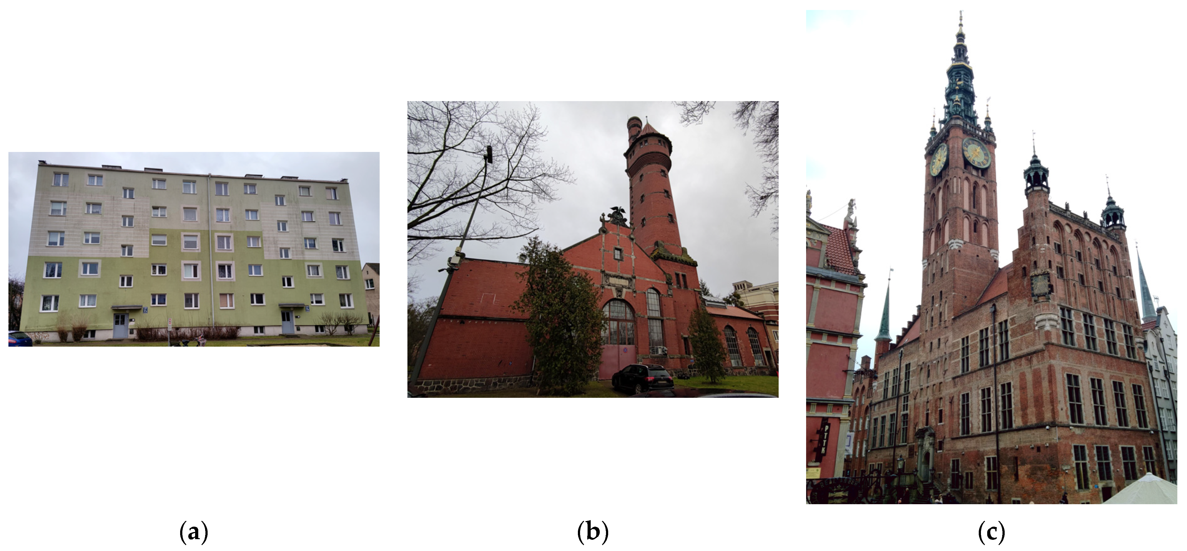
Since the translucence of the sparse point clouds may make it difficult to accurately establish the detailed surface of each object, the original buildings have been photographed, and the obtained images are presented in Figure 3 for reference purpose.
2.2. The Algorithm
The proposed algorithm has been created for the specific task of reconstructing simple 3D building models from sparse point clouds. It is based on several ideas first introduced by the 3D Grid conversion method [34], which performs special data preprocessing of the input point cloud, allowing for the generation of more detailed 3D meshes from sparse point clouds when using solutions such as Poisson surface reconstruction [35]. The algorithm proposed in this paper incorporates the ideas of preprocessing the input data in a way that increases the spatial regularity of the point cloud as well as dividing the data into a set of layers describing different height ranges. However, the proposed new algorithm uses its own dedicated method for surface reconstruction based on identifying border edges depicting the object silhouette at different height ranges. The general pipeline of this algorithm is presented in Figure 4, while the detailed description of each step is provided below.
The first step of the proposed approach consists of increasing the spatial regularity of the input data and reducing its complexity. For this reason, the entire point cloud is divided along the vertical axis into a set of layers, where each layer represents a certain height range. Then, a set of operations are applied to each layer in the following order:
- Every point in the layer is assigned to a single sector of a regular two-dimensional array projected onto the horizontal plane.
- The number of points for each non-empty 2D sector is reduced in the following way: the height of every point lying within the sector borders is compared to the average height of the entire level. The one point that is closest to the average level height on the vertical axis is preserved, while all the other members of this sector are removed from the point cloud.
- All points are moved along the vertical axis to match the average height of the entire layer. This is performed in order to achieve more regular surfaces in the final steps of the algorithm.
A sample result of performing the aforementioned steps is shown in Figure 5.
The next step is to generate a set of border edges that will describe the silhouettes of objects represented by the point cloud at different height ranges. First, the contents of each layer are split into distinct groups of connected points, which is performed using an iterative method. Next, the Delaunay triangulation method is applied to each distinct group of points in order to generate a set of temporary meshes, which are used as a basis for obtaining the desired border edges. If an edge is a part of no more than a single triangle, it is added to the result graph of the current processing step. However, this graph is not guaranteed to have the form of a circular list. For this reason, the following procedure is performed to detect inner cycles and remove loose edges. First, the starting edge of the circular list is selected based on the following criteria: one of its points must have the highest value on the depth axis for this group. If this point is connected to more than one edge, then the best edge is chosen based on the highest value of its other point on the horizontal axis. Then, the algorithm travels through every possible path until one of the three possible scenarios occurs:
- The current path ends with a dead end. In this case, the algorithm returns to the last known split, detaches the last traversed path from the results, and continues with another path.
- The path leads to the starting edge, completing the cycle. This path is selected as the result of the current step, and the remaining edges are removed from the graph.
- The current path leads back to one of the previous edges but not directly to the starting edge. In this case, this path is removed the same way as a dead-end path described in the first scenario.
A flowchart of the circular path selection process is presented in Figure 6.
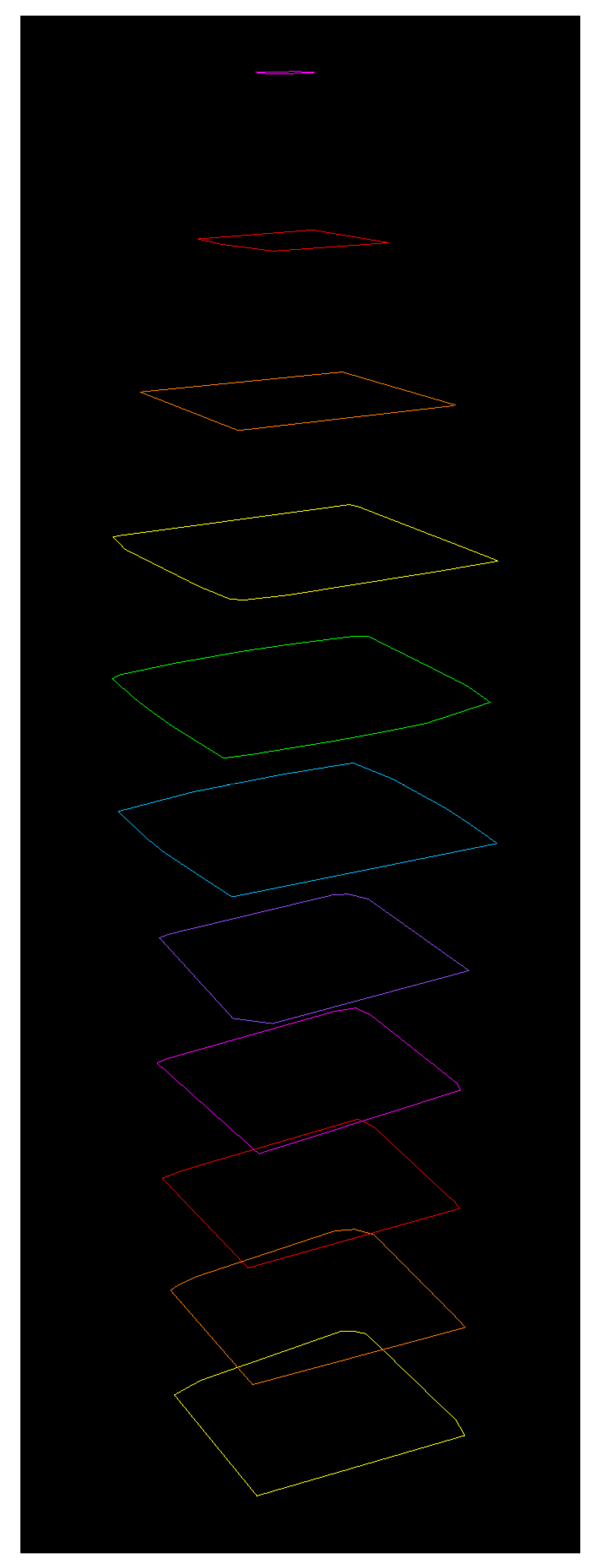
A sample set of border edges generated via path selection is shown in Figure 7.
Finally, the circular lists of edges are used as a base for creating a triangulated mesh. This is completed in three steps:
- The first set of walls is generated between pairs of layers. For each graph in an upper layer, every pair of neighbor points on the upper level is used as a base for creating a triangle, while the third required point is selected from the lower layer. The third point is always selected based on its distance from the average position of the points in the current pair: the smaller, the better.
- The gaps between pairs of layers are filled, but this time, each triangle is based on a single point from the upper layer and two neighbor points from the lower layer.
- The remaining gaps are filled by first selecting border edges within each triangulated surface and applying Delaunay triangulation to them.
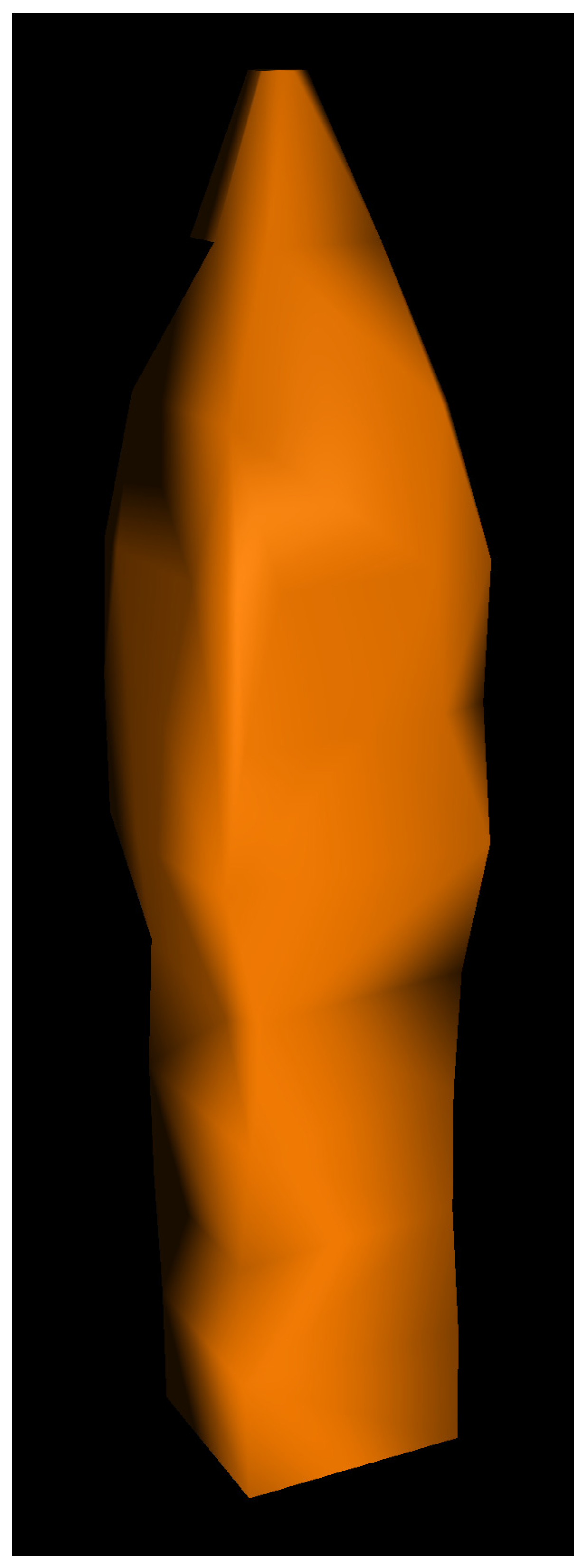
A sample result of using this procedure is shown in Figure 8.
2.3. Quantifying Algorithm Performance
The performance of the proposed method has been tested on several real-world datasets of varying quality and complexity, which have been described in the previous section. The quality of the shapes produced by the proposed method has been compared with the output of existing data-driven and model-driven reconstruction methods represented by Point2Mesh, Delaunay 2.5D algorithm (implemented by CloudCompare), and PolyFit. The algorithm performance has been tested by measuring the processing time as well as Central Processing Unit (CPU) and Random Access Memory (RAM) usage on a machine equipped with an Intel Core i7-8750H CPU with 12 logical processors operating at 2.20 GHz, 16 GB RAM, NVIDIA GeForce RTX 2070 Graphics Processing Unit (GPU) with 8 GB GDDR6 memory and a 64-bit Operating System (Windows 10 Home/Linux Mint 20.1). The measured values represent the total data processing time, including all phases of the evaluated algorithm as well as mesh simplification (if applicable).
The quantitative assessment of building reconstruction offered by the analyzed algorithms has been tested by using two different metrics: model completeness and model noisiness. Model completeness is obtained by calculating the distance from each point in the cloud to the nearest triangle in the reconstructed model R with the use of CloudCompare [36]. The lower the absolute values of the distances, the closer the reconstructed model R is to the point cloud on which it is based. However, because only the closest triangles of model R are analyzed, the metric will produce high ratings for noisy models in which some triangles are close to the reference point cloud, but others are not. As a result of this, the secondary metric has been used to assess model noisiness by computing the Hausdorff Distance [37] between the reconstructed model R and the high-poly ground truth model G, as inspired by the evaluation methodology proposed by Seitz et al. [38]. In this method, the quality of the reconstructed model may be quantified as the average and largest distances between the vertices of model R and the nearest vertices of model G. For a properly reproduced model, the values of these distances should be as small as possible. This type of quantitative assessment requires the presence of high-quality LOD3 reference models of the structures represented by each analyzed dataset. These have been constructed manually, using the original building plans (where available) as well as in situ measurements. An exception is the Gdansk Town Hall building, for which neither plans nor an accurate 3D model are publicly available. Moreover, the Town Hall’s placement at the intersection of two relatively narrow streets and the fact that two of its walls are connected to neighboring buildings make the manual construction of such a model (e.g., photogrammetrically) particularly difficult and error-prone.
2.4. Algorithm Parameters
Since Point2Mesh required that an initial mesh is provided, for each shape, the convex hull was created from the point cloud, with the target number of faces set to 5000. Additionally, it was required that surface normals were estimated for the point cloud, which was completed with MeshLab [39]. Since the available Point2Mesh implementation requires significant amounts of GPU memory, the number of iterations was limited to 1000. Finally, since the complexity of the reconstructed meshes was very high when compared to the results obtained with other methods, the number of triangles in each model was reduced ten-fold with the use of Fast-Quadric-Mesh-Simplification [40].
For the Delaunay 2.5D triangulations, the complexity of the reconstructed meshes was even higher than the Point2Mesh results; therefore, the number of triangles in each model was reduced 100 times.
PolyFit required providing additional input in the form of planar segments, which were extracted from the point clouds with Mapple [41]. Unless otherwise stated, the RANSAC parameters used for extracting planar segments from point clouds were the following:
Minimum Support: 350
Distance Threshold: 0.005
Bitmap Resolution: 0.02
Normal Threshold: 0.8
Overlook Probability: 0.001
For the face selection process, the following settings were used:
Fitting weight λf: 0.46
Coverage weight λc: 0.27
Complexity weight λm: 0.27
A complete explanation of all steps of the PolyFit algorithm is given by Nan and Wonka in [24].
3. Results
The residential building has the simplest structure of all the real-world datasets, and therefore, all analyzed algorithms should theoretically provide their best results for it. However, at the same time, it is the smallest of all analyzed structures and therefore consists of the least points. In order to use PolyFit on this dataset, a much smaller value for RANSAC Minimum Support was needed, which was set to 1, as for larger values, the reconstruction process did not create any surfaces. A comparison of the reconstruction performance by the proposed method, PolyFit, Point2Mesh, and Delaunay 2.5D for the residential building dataset is shown in Figure 9.
The Mechanical Laboratory building has a more advanced structure, with an irregularly shaped tower protruding from one of its walls. The results of its reconstruction by the proposed method, PolyFit, Point2Mesh, and Delaunay 2.5D are shown in Figure 10.
The Town Hall building is not only the most complex of the analyzed structures, with several towers, a glass-covered courtyard, and various ornaments, but it also contains large gaps in places where it connects to neighboring buildings. Therefore, it represents a worst-case scenario for all analyzed reconstruction methods. Figure 11 presents how the proposed method, PolyFit, Point2Mesh, and Delaunay 2.5D managed to reconstruct this building.
The performance of the analyzed algorithms in the form of processing time is presented in Table 1. The given values represent the total time taken from the ingestion of the input point clouds to producing simplified meshes. The CPU and RAM usage is presented in Table 2. Since Point2Mesh uses CUDA, GPU memory usage is also shown for this method.
As can be seen, the proposed algorithm and the Delaunay triangulation both offered the best processing performance while also maintaining relatively low CPU usage. Moreover, the proposed algorithm achieved the shortest processing time overall across all analyzed datasets, reaching near real-time execution. The Delaunay 2.5D algorithm achieved second place overall, although it should be noted that the majority of processing time and cost of this method was taken by mesh simplification. In contrast, Point2Mesh required several minutes to complete a single task, while also allocating significantly large amounts of RAM and GPU memory. PolyFit performed several times faster than Point2Mesh although at the cost of much larger CPU usage.
Table 3 presents the results of the reconstruction quality analysis of all tested algorithms, which was performed by calculating the distance between each point in the cloud and the closest triangle of the reconstructed model. This metric is best used to reflect whether the analyzed reconstruction method managed to properly reproduce the general shape of the original structure. As mentioned earlier, the lower the absolute value in each category, the closer the reconstructed mesh is to the point cloud on which it is based. Negative values mean that the model undershoots, i.e., its surface lies below the points in the cloud. Similarly, values larger than zero mean that the model forms an outer shell over the point cloud.
As it can be seen, when the general shape of the reconstructed building is concerned, the results are heavily dependent on the input data. For the residential building dataset, the proposed algorithm obtained the best results in all categories, although the Delaunay method came in close second in terms of mean distance and standard deviation. For the Mechanical Laboratory building dataset, Point2Mesh obtained the best spread values, Delaunay 2.5D outperformed other methods in terms of mean distance and standard deviation, while the proposed method came in third in most categories. For the Town Hall dataset, the best overall results were obtained by Point2Mesh, while the proposed method came in second in terms of maximum spread value and third in terms of minimum spread value and standard deviation.
Table 4 presents the mesh noisiness results calculated between each vertex of the reconstructed model R and the closest vertex of ground truth model G. In contrast to the previous method, this metric will assign low scores to noisy models; however, because the distance is measured from model R to model G, it will not tell us whether the entire shape of the original object has been properly reconstructed. This is reflected by the scores calculated for the PolyFit reconstruction of the residential building dataset. The algorithm only managed to reconstruct the roof part of the building; however, the shape of the produced surface is close to how it looks in the reference model. As a consequence, this reconstruction achieved good scores from the second metric (which measures the noise of the reconstructed model) and low scores from the first metric (which assesses the general accuracy of the reconstructed model). As mentioned earlier, the Gdansk Town Hall building was omitted in the calculation due to the lack of the ground truth model R.
When model noisiness is concerned, the proposed method achieved the lowest mean distance for the Mechanical Laboratory building dataset while also taking second place in both categories for the Residential building dataset. Point2Mesh achieved the lowest maximum distance for the Mechanical Laboratory building dataset but at the same time obtained the worst results in both categories for the Residential building dataset. Interestingly, the Delaunay 2.5D method obtained the best results for the Residential building dataset while performing rather poorly in case of the Mechanical Laboratory building dataset.
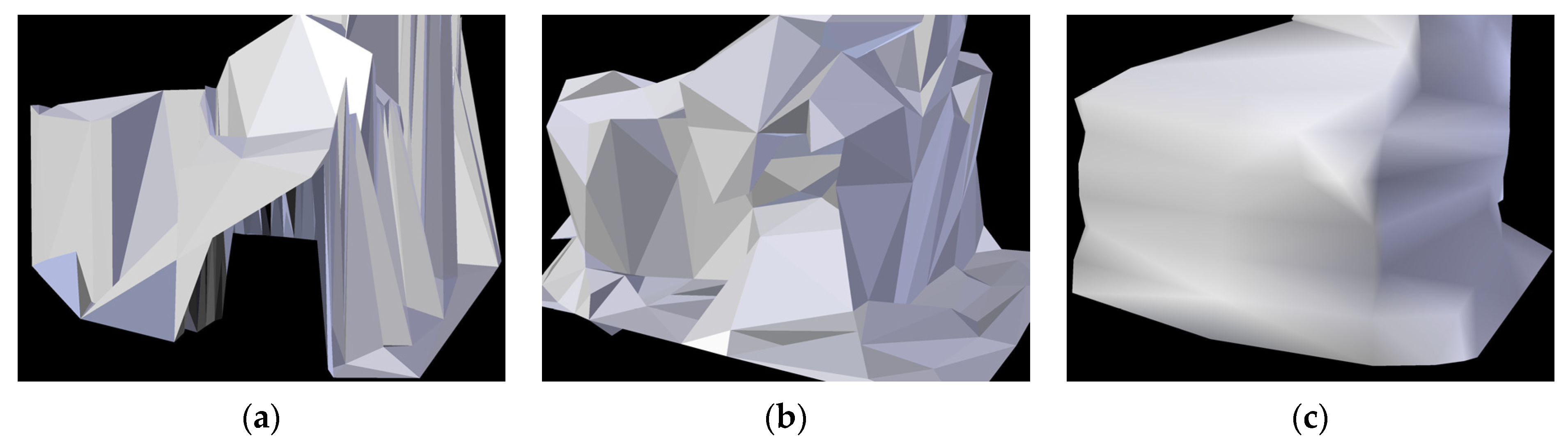
It should be noted that while the employed model completeness metric should, in general, penalize the existence of gaps in the reconstructed meshes, it will not do so if the gaps also exist in the point cloud as a result of incomplete surface scanning. This means that in the case of sparse point clouds, obtaining a good reconstruction score via the cloud-to-mesh distance metric does not guarantee that the model faithfully represents the original object. An example of this is the Delaunay 2.5D algorithm, which received some of the best scores in mean distance and standard deviation while producing incomplete models (see Figure 12).
4. Discussion
The performance and reconstruction quality of the proposed method has been tested on several sparse point clouds of variable quality, representing buildings of various complexity. For the residential building, which has the simplest shape, the proposed method achieved satisfactory results by reproducing the original building’s rectangular cuboid shape. In comparison, Delaunay 2.5D obtained good results for the roof segment, but the recreated mesh contains a significant number of gaps in the lower parts of the building. Point2Mesh properly reproduced the general shape of the building; however, it introduced a lot of polygon noise. Some of this noise could be removed by means of shape simplification; however, the result remains worse than the proposed method. PolyFit produced even worse results, only properly reconstructing the roof of the building. This is likely caused by the small number of vertices on the walls, as (similarly to Point2Mesh), PolyFit works best with dense point clouds.
The Mechanical Laboratory represents a more complex shape, which is represented by a significantly denser point cloud. For this dataset, the proposed method also achieved a satisfactory result; however, Point2Mesh produced a shape of comparable quality, while Delaunay 2.5D obtained better representation of the roof but once again introduced a large number of gaps in the lower parts of the building. The denser point cloud enabled PolyFit to achieve better reconstruction results than in the previous example; however, the obtained shape does not properly represent the original building.
Finally, the Gdansk Town Hall dataset represents the most complex of all reconstructed shapes. The original building, constructed in the 15th century and later expanded, is a mix of gothic and renaissance architectures with various ornaments. Moreover, although the density of the point cloud is similar to the one representing the Mechanical Laboratory, the dataset has not been carefully preprocessed and contains parts of adjacent buildings as well as large gaps in places of shared walls. Regardless, the proposed method produced an acceptable result, properly representing the general shape of the building, especially its main tower, although with some oversimplification of its roof. Delaunay 2.5D and Point2Mesh obtained similar results, producing substantially noisier meshes but with more detailed roofs. In addition, Delaunay 2.5D did not close the gaps in the original point cloud. Once again, PolyFit only managed to reconstruct part of the roof, excluding the tower and the entire lower part of the Town Hall. In general, the model produced by the proposed method is of acceptable quality for applications such as flood hazard modeling, which require a general three-dimensional shape of the building. A more accurate representation of this structure would need to be created manually, as none of the tested methods managed to reconstruct neither the original structure of the roof nor any of the four smaller towers in the center.
On the whole, the proposed algorithm has been shown to produce satisfying results both when reconstructing simple as well as more complex shapes. The employed vertical dataset segmentation has shown to provide good resilience against incomplete datasets, provided that the information regarding the original shape of the structure is available at some level of the point cloud. In general, the denser and more detailed the input point cloud, the better the results that have been produced by the existing methods. PolyFit had a tendency to accurately reconstruct uniform parts of the original building such as roofs or walls, while Point2Mesh usually properly recovered the general shape of the building but also introduced a lot of polygon noise, which could only partially be removed by shape simplification. Delaunay 2.5D offered good results when reconstructing roofs but behaved worse for parts such as walls and towers. Moreover, it appears that the method is not very resilient to gaps in the source point cloud, as every mesh it has generated was incomplete in this aspect.
In terms of quantitative reconstruction assessment scores, a summary of performance results of different surface reconstruction methods is presented in Table 5, which is ranked from I (best) to IV (worst) based on the sum of absolute values obtained in each category. It can be seen that the proposed method offers good uniformity (represented by low spread value) and minimum noisiness in the reconstructed meshes while also requiring the least amount of processing time and CPU usage and maintaining low memory usage. Point2Mesh offers better results in terms of model completeness but at the cost of the highest amount of model noisiness as well as processing time and memory usage. PolyFit obtained the worst overall results except for model noisiness. The Delaunay 2.5D algorithm offers good to average results in all categories while maintaining the lowest memory requirements. However, it needs to be noted that both PolyFit and Delaunay 2.5D did not produce complete models, and this fact should be taken into account when analyzing the results.
In financial terms, the presented algorithm enables automated reconstruction of city models from sparse point clouds which are freely and publicly available for many areas in the world, particularly in the EU and the USA. In consequence, a LOD2-level mesh representation of city structures for such areas may be obtained at no additional cost, in particular because the hardware requirements for the presented method are so low that it may be executed on virtually any desktop-class computer produced during the last decade.
While the proposed algorithm has shown to offer competitive performance and reconstruction quality compared to existing methods, it should be noted that currently, it does not guarantee manifold nor watertight reconstructions, which means that the produced buildings cannot be used e.g., for simulations of energy conservation. However, this should not be a problem, as such analyses require high-quality building models that may only be obtained via terrestrial lidar scanning, photogrammetry, or manual modeling [42]. Models produced by the proposed method may be used for a variety of purposes, such as large-scale modeling and simulation of flooding, where (in comparison to commonly used LOD1 datasets), their more detailed representation of original building shapes may allow for more accurate calculation of the percentage in which a building will be covered in water [43], or for an optimized preview of separately available high-resolution datasets [44]. Moreover, the proposed algorithm may also be used for the purpose of generating lower levels of detail for high-quality models obtained using other techniques [45].
5. Conclusions
This paper presents a novel method of 3D building reconstruction optimized for working with sparse and incomplete point clouds, which are usually produced by airborne lidar scanning. The proposed method employs data segmentation, silhouette extraction, and triangulation in order to provide simplified 3D models that properly represent the shape of the original building. The performance of the proposed algorithm has been tested on several sparse point clouds of variable quality, representing buildings of various complexity, and compared to results produced by existing methods represented by PolyFit, Point2Mesh, and Delaunay 2.5D triangulation. These results have been assessed using quantitative methods based on calculating point cloud to mesh distance as well as computing the Hausdorff distance between the reconstructed model and the ground truth model. The results have shown that the proposed method performs well both in terms of reconstructing the general shape of the building and in producing a uniform and noise-free model while also maintaining very low processing time and cost. Tests have shown that the proposed method successfully reconstructs simple as well as complex buildings from sparse point clouds obtained via airborne lidar scanning and thus may be used for the automatic processing of such datasets, provided that they have been properly extracted from the source point cloud. As a result of this, the proposed algorithm provides a cost-effective means of producing 3D city models from freely available datasets. Moreover, the method is particularly useful for generating representations of non-uniform shapes, which may be commonly found, e.g., in buildings from the renaissance era or ornate places of worship such as cathedrals.
Further improvements of the proposed method will concentrate on more accurate silhouette generation for distinct surfaces as well as providing watertight reconstructions. The former may be achieved by comparing the temporary meshes obtained with Delaunay triangulation against the input point cloud in order to improve the current mechanism of border edges selection. The latter can be achieved by proper selection and removal of non-manifold geometry during the surface reconstruction step.
Funding
This research received no external funding.
Data Availability Statement
The data used in this study are available upon request.
Conflicts of Interest
The author declares no conflict of interest.
References
- La Russa, F.M.; Galizia, M.; Santagati, C. Remote sensing and city information modeling for revealing the complexity of historical centers. Int. Arch. Photogramm. Remote Sens. Spat. Inf. Sci. 2021, 46, 367–374. [Google Scholar] [CrossRef]
- Trizio, I.; Marra, A.; Savini, F.; Fabbrocino, G. Survey methodologies and 3D modelling for conservation of historical masonry bridges. ISPRS Ann. Photogramm. Remote Sens. Spat. Inf. Sci. 2021, 8, 163–170. [Google Scholar] [CrossRef]
- Riveiro, B.; Lindenbergh, R. Laser Scanning: An Emerging Technology in Structural Engineering; CRC Press: Boca Raton, FL, USA, 2019. [Google Scholar]
- Vamvakeridou-Lyroudia, L.S.; Chen, A.S.; Khoury, M.; Gibson, M.J.; Kostaridis, A.; Stewart, D.; Wood, M.; Djordjevic, S.; Savic, D. Assessing and visualising hazard impacts to enhance the resilience of Critical Infrastructures to urban flooding. Sci. Total Environ. 2019, 707, 136078. [Google Scholar] [CrossRef] [PubMed]
- Ying, S.; Guo, R.; Li, L.; He, B. Application of 3D GIS to 3D Cadastre in Urban Environment. 2012. Available online: https://repository.tudelft.nl/islandora/object/uuid:27cf8c1f-d5e5-409e-9425-dcce26391385 (accessed on 16 February 2022).
- Kulawiak, M.; Lubniewski, Z. SafeCity—A GIS-based tool profiled for supporting decision making in urban development and infrastructure protection. Technol. Forecast. Soc. Chang. 2014, 89, 174–187. [Google Scholar] [CrossRef]
- Gröger, G.; Kolbe, T.H.; Nagel, C.; Häfele, K.-H. OGC City Geography Markup Language (CityGML) Encoding Standard. Open Geospatial Consortium. 2012. Available online: https://www.ogc.org/standards/citygml (accessed on 11 November 2021).
- INSPIRE Geoportal. Available online: https://inspire-geoportal.ec.europa.eu (accessed on 25 November 2021).
- Hackel, T.; Wegner, J.D.; Schindler, K. Contour detection in unstructured 3D point clouds. In Proceedings of the IEEE Conference on Computer Vision and Pattern Recognition 2016, Las Vegas, NV, USA, 27–30 June 2016; pp. 1610–1618. [Google Scholar]
- Nevatia, R.; Price, K. Automatic and interactive modeling of buildings in urban environments from aerial images. In Proceedings of the International Conference on Image Processing, Rochester, NY, USA, 22–25 September 2002. [Google Scholar] [CrossRef]
- Jayaraj, P.; Ramiya, A.M. 3D citygml building modelling from lidar point cloud data. ISPRS—Int. Arch. Photogramm. Remote Sens. Spat. Inf. Sci. 2018, XLIIp-5, 175–180. [Google Scholar] [CrossRef] [Green Version]
- 3dfier. Available online: https://github.com/tudelft3d/3dfier (accessed on 10 November 2021).
- LAStools. Available online: https://rapidlasso.com/lastools/ (accessed on 14 November 2019).
- citygml4j. Available online: https://github.com/citygml4j/citygml4j (accessed on 10 November 2021).
- CloudCompare Wiki: Surface between Two Polylines. Available online: https://www.cloudcompare.org/doc/wiki/index.php?title=Mesh%5CSurface_between_two_polylines (accessed on 16 February 2022).
- Maptek PointStudio. Available online: https://www.maptek.com/products/pointstudio/?utm_source=products-i-site-i-site_studio.html&utm_medium=301 (accessed on 16 February 2022).
- Hanocka, R.; Metzer, G.; Giryes, R.; Cohen-Or, D. Point2mesh: A self-prior for deformable meshes. arXiv 2020, arXiv:2005.11084. [Google Scholar] [CrossRef]
- Delaunay, B. Sur la sphere vide. Izv. Akad. Nauk SSSR 1934, 7, 1–2. [Google Scholar]
- CloudCompare Wiki: Delaunay 2.5D (XY Plane). Available online: https://www.cloudcompare.org/doc/wiki/index.php?title=Mesh%5CDelaunay_2.5D_(XY_plane) (accessed on 16 February 2022).
- CloudCompare Wiki: Delaunay 2.5D (Best Fit Plane). Available online: https://www.cloudcompare.org/doc/wiki/index.php?title=Mesh%5CDelaunay_2.5D_(best_fit_plane) (accessed on 16 February 2022).
- Buyukdemircioglu, M.; Kocaman, S.; Isikdag, U. Semi-automatic 3D city model generation from large-format aerial images. ISPRS Int. J. Geo-Inf. 2018, 7, 339. [Google Scholar] [CrossRef] [Green Version]
- Bittner, K.; D’Angelo, P.; Körner, M.; Reinartz, P. DSM-to-LoD2: Spaceborne stereo digital surface model refinement. Remote Sens. 2018, 10, 1926. [Google Scholar] [CrossRef] [Green Version]
- Yang, B.; Lee, J. Improving accuracy of automated 3-D building models for smart cities. Int. J. Digit. Earth 2017, 12, 209–227. [Google Scholar] [CrossRef]
- Nan, L.; Wonka, P. Polyfit: Polygonal surface reconstruction from point clouds. In Proceedings of the IEEE International Conference on Computer Vision, Venice, Italy, 22–29 October 2017; pp. 2353–2361. [Google Scholar]
- Hensel, S.; Goebbels, S.; Kada, M. Facade reconstruction for textured lod2 citygml models based on deep learning and mixed integer linear programming. ISPRS Ann. Photogramm. Remote Sens. Spat. Inf. Sci. 2019, IV-2/W5, 37–44. [Google Scholar] [CrossRef] [Green Version]
- Kanayama, T.; Mineushiro, T.; Date, H.; Kanai, S. Segmentation and LOD model generation of buildings from MMS point clouds of urban area. J. Jpn. Soc. Precis. Eng. 2019, 85, 912–918. [Google Scholar] [CrossRef] [Green Version]
- Nurunnabi, A.; Belton, D.; West, G. Robust segmentation in laser scanning 3D point cloud data. In Proceedings of the 2012 International Conference on Digital Image Computing Techniques and Applications (DICTA), Fremantle, WA, Australia, 3–5 December 2012. [Google Scholar]
- Wold, S.; Esbensen, K.; Geladi, P. Principal component analysis. Chemom. Intell. Lab. Syst. 1987, 2, 37–52. [Google Scholar] [CrossRef]
- Fischler, M.A.; Bolles, R.C. Random sample consensus: A paradigm for model fitting with applications to image analysis and automated cartography. Commun. ACM 1981, 24, 381–395. [Google Scholar] [CrossRef]
- Nys, G.-A.; Poux, F.; Billen, R. CityJSON Building generation from airborne LiDAR 3D point clouds. ISPRS Int. J. Geo-Inf. 2020, 9, 521. [Google Scholar] [CrossRef]
- Poux, F.; Billen, R. Voxel-based 3D point cloud semantic segmentation: Unsupervised geometric and relationship featuring vs. deep learning methods. ISPRS Int. J. Geo-Inf. 2019, 8, 213. [Google Scholar] [CrossRef] [Green Version]
- Topographic Data Quality Levels (QLs). Available online: https://www.usgs.gov/3d-elevation-program/topographic-data-quality-levels-qls (accessed on 16 February 2022).
- Geoportal Krajowy. Available online: https://mapy.geoportal.gov.pl/imap/Imgp_2.html (accessed on 26 November 2021).
- Kulawiak, M.; Lubniewski, Z. Improving the accuracy of automatic reconstruction of 3D complex buildings models from airborne lidar point clouds. Remote Sens. 2020, 12, 1643. [Google Scholar] [CrossRef]
- Kazhdan, M.; Bolitho, M.; Hoppe, H. Poisson surface reconstruction. In Proceedings of the 4th Eurographics Symposium on Geometry Processing, Cagliari, Italy, 26–28 June 2006; pp. 61–70. [Google Scholar]
- CloudCompare Wiki: Cloud-to-Mesh Distance. Available online: http://www.cloudcompare.org/doc/wiki/index.php?title=Cloud-to-Mesh_Distance (accessed on 16 February 2022).
- Cignoni, P.; Rocchini, C.; Scopigno, R. Metro: Measuring error on simplified surfaces. Comput. Graph. Forum 1998, 17, 167–174. [Google Scholar] [CrossRef] [Green Version]
- Seitz, S.M.; Curless, B.; Diebel, J.; Scharstein, D.; Szeliski, R. A comparison and evaluation of multi-view stereo reconstruction algorithms. In Proceedings of the 2006 IEEE computer society conference on computer vision and pattern recognition (CVPR'06), New York, NY, USA, 17–22 June 2006; Volume 1, pp. 519–528. [Google Scholar]
- Cignoni, P.; Callieri, M.; Corsini, M.; Dellepiane, M.; Ganovelli, F.; Ranzuglia, G. MeshLab: An Open-source mesh processing tool. In Proceedings of the Eurographics Italian Chapter Conference, Salerno, Italy, 2–4 July 2008. [Google Scholar]
- Fast-Quadric-Mesh-Simplification. Available online: https://github.com/sp4cerat/Fast-Quadric-Mesh-Simplification (accessed on 25 November 2021).
- Mapple. Available online: https://3d.bk.tudelft.nl/liangliang/software.html (accessed on 25 November 2021).
- Cai, Y.; Fan, L. An efficient approach to automatic construction of 3D watertight geometry of buildings using point clouds. Remote Sens. 2021, 13, 1947. [Google Scholar] [CrossRef]
- Zhi, G.; Liao, Z.; Tian, W.; Wu, J. Urban flood risk assessment and analysis with a 3D visualization method coupling the PP-PSO algorithm and building data. J. Environ. Manag. 2020, 268, 110521. [Google Scholar] [CrossRef]
- Kulawiak, M.; Kulawiak, M. Application of Web-GIS for dissemination and 3D visualization of large-volume LIDAR data. In The Rise of Big Spatial Data; Springer: Cham, Switzerland, 2017; pp. 1–12. [Google Scholar] [CrossRef]
- Kulawiak, M.; Kulawiak, M.; Lubniewski, Z. Integration, processing and dissemination of LiDAR data in a 3D Web-GIS. ISPRS Int. J. Geo-Inf. 2019, 8, 144. [Google Scholar] [CrossRef] [Green Version]
Figure 1.
Datasets used in the study: (a) Residential building; (b) Gdansk University of Technology Mechanical Laboratory building; (c) Gdansk Town Hall.
Figure 1.
Datasets used in the study: (a) Residential building; (b) Gdansk University of Technology Mechanical Laboratory building; (c) Gdansk Town Hall.

Figure 2.
The location of largest gaps in the datasets used in the study (marked in red): (a) Residential building; (b) Gdansk University of Technology Mechanical Laboratory building; (c) Gdansk Town Hall.
Figure 2.
The location of largest gaps in the datasets used in the study (marked in red): (a) Residential building; (b) Gdansk University of Technology Mechanical Laboratory building; (c) Gdansk Town Hall.

Figure 3.
Photographs representing the real-world objects on which the point clouds used in this study were based: (a) Residential building; (b) Gdansk University of Technology Mechanical Laboratory building; (c) Gdansk Town Hall.
Figure 3.
Photographs representing the real-world objects on which the point clouds used in this study were based: (a) Residential building; (b) Gdansk University of Technology Mechanical Laboratory building; (c) Gdansk Town Hall.

Figure 4.
The main steps performed by the proposed algorithm.

Figure 5.
Comparison of the original point cloud and the result of converting it into a set of simplified layers: (a) Original lidar point cloud; (b) Simplified point cloud, divided into a set of layers.
Figure 5.
Comparison of the original point cloud and the result of converting it into a set of simplified layers: (a) Original lidar point cloud; (b) Simplified point cloud, divided into a set of layers.

Figure 6.
The process of circular path selection performed during the silhouette generation step.

Figure 7.
A set of border edges created on the basis of the simplified point cloud.

Figure 8.
Building mesh obtained from the simplified point cloud by the proposed algorithm.

Figure 9.
Comparison of reconstruction performance for the residential building dataset: (a) The proposed method; (b) PolyFit; (c) Point2Mesh; (d) Delaunay 2.5D.
Figure 9.
Comparison of reconstruction performance for the residential building dataset: (a) The proposed method; (b) PolyFit; (c) Point2Mesh; (d) Delaunay 2.5D.

Figure 10.
Comparison of reconstruction performance for the Mechanical Laboratory dataset: (a) The proposed method; (b) PolyFit; (c) Point2Mesh; (d) Delaunay 2.5D.
Figure 10.
Comparison of reconstruction performance for the Mechanical Laboratory dataset: (a) The proposed method; (b) PolyFit; (c) Point2Mesh; (d) Delaunay 2.5D.

Figure 11.
Comparison of reconstruction performance for the Town Hall dataset: (a) The proposed method; (b) PolyFit; (c) Point2Mesh; (d) Delaunay 2.5D.
Figure 11.
Comparison of reconstruction performance for the Town Hall dataset: (a) The proposed method; (b) PolyFit; (c) Point2Mesh; (d) Delaunay 2.5D.

Figure 12.
Comparison of models reconstructed from the Mechanical Laboratory building dataset using different methods, shown from a perspective where a large gap is present in the point cloud: (a) Delaunay 2.5D; (b) Point2Mesh; (c) The proposed method.
Figure 12.
Comparison of models reconstructed from the Mechanical Laboratory building dataset using different methods, shown from a perspective where a large gap is present in the point cloud: (a) Delaunay 2.5D; (b) Point2Mesh; (c) The proposed method.


Table 1.
Processing time of different surface reconstruction methods. Bold values mean better results in a given category.
Table 1.
Processing time of different surface reconstruction methods. Bold values mean better results in a given category.
| Method | Residential Building | Mechanical Laboratory | Town Hall |
|---|---|---|---|
| Proposed algorithm | 0.1 s | 1.2 s | 0.8 s |
| Point2Mesh (with decimation) | 5 min 57.2 s | 6 min 34.7 s | 6 min 19.2 s |
| PolyFit | 1.66 s | 47.8 s | 9.9 s |
| Delaunay 2.5D (with decimation) | 0.2 s | 0.8 s | 2.1 s |
Table 2.
Processing cost of different surface reconstruction methods. Bold values mean better results in a given category.
Table 2.
Processing cost of different surface reconstruction methods. Bold values mean better results in a given category.
| Method | CPU [%] | RAM [MB] | GPU memory [MB] |
|---|---|---|---|
| Proposed algorithm | 6–9 (avg. 7.5) | 20 | - |
| Point2Mesh (with decimation) | 8 | 2100–2200 (avg. 2150) | 4781–4803 |
| PolyFit | 2–31 (avg. 16.5) | 8–125 (avg. 66.5) | - |
| Delaunay 2.5D (with decimation) | 4–18 (avg. 11) | 3–26 (avg. 14.5) | - |
Table 3.
Results of point cloud to mesh distance calculated for meshes reconstructed with different methods. Bold values mean better results in a given category.
Table 3.
Results of point cloud to mesh distance calculated for meshes reconstructed with different methods. Bold values mean better results in a given category.
| Value | Method | Residential Building [cm] | Mechanical Laboratory [cm] | Town Hall [cm] |
|---|---|---|---|---|
| Minimum spread value | Proposed algorithm | −117.09 | −747.52 | −1175.84 |
| Point2Mesh (after decimation) | −213.62 | −540.46 | −676.74 | |
| PolyFit | −1582.20 | −2024.38 | −2122.36 | |
| Delaunay (after decimation) | −662.58 | −580.55 | −848.94 | |
| Maximum spread value | Proposed algorithm | 92.64 | 745.69 | 718.84 |
| Point2Mesh (after decimation) | 206.61 | 543.78 | 694.58 | |
| PolyFit | 1617.78 | 1989.25 | 5189.39 | |
| Delaunay (after decimation) | 381.16 | 567.32 | 822.52 | |
| Mean distance | Proposed algorithm | −2.32 | −144.80 | −227.49 |
| Point2Mesh (after decimation) | −67.05 | 12.47 | −22.88 | |
| PolyFit | −85.39 | −18.35 | 88.86 | |
| Delaunay (after decimation) | −2.71 | −0.01 | 4.7 | |
| Standard deviation | Proposed algorithm | 29.38 | 242.72 | 236.47 |
| Point2Mesh (after decimation) | 37.51 | 66.04 | 80.54 | |
| PolyFit | 419.62 | 293.52 | 829.79 | |
| Delaunay (after decimation) | 34.14 | 23.50 | 94.25 |
Table 4.
Noisiness of meshes reconstructed with different methods, depicted as distances between vertices of models R and G. Bold values mean better results in a given category.
Table 4.
Noisiness of meshes reconstructed with different methods, depicted as distances between vertices of models R and G. Bold values mean better results in a given category.
| Value | Method | Residential Building [cm] | Mechanical Laboratory [cm] |
|---|---|---|---|
| Maximum distance | Proposed algorithm | 73.16 | 1136.18 |
| Point2Mesh (after decimation) | 712.06 | 880.21 | |
| PolyFit | 251.59 | 941.20 | |
| Delaunay 2.5D (after decimation) | 66.36 | 1244.63 | |
| Mean distance | Proposed algorithm | 19.68 | 62.06 |
| Point2Mesh (after decimation) | 124.68 | 93.18 | |
| PolyFit | 44.99 | 143.86 | |
| Delaunay 2.5D (after decimation) | 10.94 | 119.45 |
Table 5.
Overall performance of different surface reconstruction methods.
| Metric | Proposed Algorithm | Point2Mesh | PolyFit | Delaunay 2.5D | |
|---|---|---|---|---|---|
| Model completeness | Minimum spread value | II | I | IV | III |
| Maximum spread value | II | I | IV | III | |
| Mean distance | IV | II | III | I | |
| Standard deviation | III | II | IV | I | |
| Model noisiness | Maximum distance | II | IV | I | III |
| Mean distance | I | IV | III | II | |
| Hardware requirements | Processing time | I | IV | III | II |
| CPU usage | I | II | IV | III | |
| Memory usage | II | IV | III | I | |
Publisher’s Note: MDPI stays neutral with regard to jurisdictional claims in published maps and institutional affiliations. |
© 2022 by the author. Licensee MDPI, Basel, Switzerland. This article is an open access article distributed under the terms and conditions of the Creative Commons Attribution (CC BY) license (https://creativecommons.org/licenses/by/4.0/).
Share and Cite
MDPI and ACS Style
Kulawiak, M. A Cost-Effective Method for Reconstructing City-Building 3D Models from Sparse Lidar Point Clouds. Remote Sens. 2022, 14, 1278. https://doi.org/10.3390/rs14051278
AMA Style
Kulawiak M. A Cost-Effective Method for Reconstructing City-Building 3D Models from Sparse Lidar Point Clouds. Remote Sensing. 2022; 14(5):1278. https://doi.org/10.3390/rs14051278
Chicago/Turabian StyleKulawiak, Marek. 2022. "A Cost-Effective Method for Reconstructing City-Building 3D Models from Sparse Lidar Point Clouds" Remote Sensing 14, no. 5: 1278. https://doi.org/10.3390/rs14051278
Note that from the first issue of 2016, this journal uses article numbers instead of page numbers. See further details here.