Granularity of Digital Elevation Model and Optimal Level of Detail in Small-Scale Cartographic Relief Presentation

Abstract

One of the key applications of digital elevation models (DEMs) is cartographic relief presentation. DEMs are widely used in mapping, most commonly in the form of contours, hypsometric tints, and hill shading. Recent advancements in the coverage, quality, and resolution of global DEMs facilitate the overall improvement of the detail and reliability of terrain-related research. At the same time, geographic problem solving is conducted in a wide variety of scales, and the data used for mapping should have the corresponding level of detail. Specifically, at small scales, intensive generalization is needed, which is also true for elevation data. With the widespread accessibility of detailed DEMs, this principle is often violated, and the data are used for mapping at scales far smaller than what is appropriate. Small-scale relief shading obtained from fine-resolution DEMs is excessively detailed and brings an unclear representation of the Earth’s surface instead of emphasizing what is important at the scale of visualization. Existing coarse-resolution global DEMs do not resolve the issue, since they accumulate the maximum possible information in every pixel, and therefore also require reduction in detail to obtain a high-quality cartographic image. It is clear that guidelines and effective principles for DEM generalization at small scales are needed. Numerous algorithms have been developed for the generalization of elevation data represented either in gridded, contoured, or pointwise form. However, the answer to the most important question—When should we stop surface simplification?—remains unclear. Primitive error-based measures such as vertical distance are not effective for cartography, since they do not account for the landform structure of the surface perceived by the map reader. The current paper approached the problem by elaborating the granularity—a newly developed property of DEMs, which characterizes the typical size of a landform represented on the DEM surface. A methodology of estimating the granularity through a landform width measure was conceptualized and implemented as software. Using the developed program tools, the optimal granularity was statistically learned from DEMs reconstructed for multiple fragments of manually drawn 1:200,000, 1:500,000, and 1:1,000,000 topographic maps covering different relief types. It was shown that the relative granularity should be 5–6 mm at the mapping scale to achieve the clearness of relief presentation typical for manually drawn maps. We then demonstrate how the granularity measure can be used effectively as a constraint during DEM generalization. Experimental results on a combination of contours, hypsometric tints, and hill shading indicated clearly that the optimal level of detail in small-scale cartographic relief presentation can be achieved by DEM generalization constrained by granularity in combination with fine DEM resolution, which facilitates high-quality rendering.

1. Introduction

Digital elevation models (DEMs) are widely used in modern cartography and GIScience. Aside from the computation of useful topographic variables, DEMs are often just visualized—to represent relief on a map. Since maps are created in a wide range of scales, appropriate generalization of DEMs is needed, otherwise relief presentation will be crowded with excessive details. Resolution and coverage of elevation data have increased dramatically over the last few decades. Current global DEMs such as the MERIT DEM [1] and the NASADEM [2] provide global or semi-global coverage of the land with a resolution of 30–90 m. Less extensive airborne LIDAR or optically derived DEMs may have resolutions from the first meters up to the first centimeters [3]. Since finer resolution is often considered to be an indicator of higher DEM quality, it is not uncommon to see small-scale maps produced from such detailed sources without generalization. However, the lack of generalization decreases the map readability and damages the visual impression.

The understanding of what is large, middle, or small scale differs between the standards adopted by national mapping agencies, academic institutions, and application areas. In this paper, the classification by Imhof [4], which was developed specifically for cartographic relief presentation, was followed. According to Imhof’s observations, scales smaller than 1:100,000 are characterized by the unavoidable necessity of generalization. The simplification of the surface represented by contour lines extends more or less over the whole map image and not only in particular places. Such scales are considered to be small. Therefore, in the current study, DEM applications for mapping at scales 1:200,000 and smaller were of interest.

Since each map scale corresponds to a specific level of detail (LoD), it can be decomposed into several components. Ruas and Bianchin [5] conceptualized the LoD of a spatial database as a combination of conceptual schema of the data, semantic resolution, geometric resolution, geometric precision, and granularity. While schema, resolution, and precision reflect the potential capacity of a database to represent the real world, the last LoD component—a granularity—defines the actual size of spatial features and elements of their shape (such as bends), which will be shown on a map. In the case of relief, such features are landforms—hills, valleys, etc., and their subordinate elements.

Relief generalization has been a well-elaborated topic since the times of traditional manual cartography. Useful recommendations can be found in specialized monographs [4,6] and official guidelines for topographic map creation published by national mapping agencies [7,8]. While such publications are quite comprehensive in describing the qualitative principles of surface simplification, they are somewhat stingy in terms of the numerical description of the desired relief granularity. For example, the linear size of surface discontinuities such as cliffs, gullies, or faults to be shown on a Russian topographic map of 1:200,000 scale must be at least 3–10 mm depending on the type of feature [7]. A recommended minimum size of colored area symbols is 4 mm${}^2$ according to Swiss Society of Cartography [8]. Still, recommendations on the minimum or typical landform size are hard to find, and usually, this size is said to be capable of reflecting the “surface features typical at mapping scale” [6].

It seems, however, that DEM granularity must be comparable to the general recommendations for representing the smallest objects, which are about the first millimeters in linear dimensions on a map. Moreover, perceiving the objects from a computer screen is usually harder than from a printed medium; therefore, this threshold can be deliberately enlarged.

This paper presents the computational approach that formalizes the determination of DEM granularity and its suitability for mapping at a certain scale. In the first stage, the computation of the granularity is elaborated through a new measure called landform width. In the next stage, the optimal granularity is statistically learned using DEMs reconstructed from topographic maps covering different terrain conditions. Experimental work was then conducted to achieve the optimal detail of cartographic relief presentation at the specified scale by DEM generalization constrained by granularity. The resistance of landform width measure to DEM upsampling was assessed in the final experiment.

The rest of the paper consists of several sections. In Section 2, an overview of the related research is presented. Section 3 and Section 4 uncover the developed methodology and its implementation. The results of the experimental work are presented in Section 5. The discussion on the limitations of the developed approach comprises Section 6. Finally, the Conclusion summarizes the most important findings of the research.

2. Related Research

The quality of digital elevation models is a frequently discussed topic in scientific research. Understanding the quality, as well as possible quality measures and their preferred values are not universal and depend on the user’s task [9]. Small-scale mapping based on DEMs is a specific task that puts the appropriate generalization in front of other quality aspects [4]. At the same time, surveys indicate that users typically express unwillingness to devote much time to evaluate the impact that DEM quality might have on their applications [10]. These conditions imply that various DEM quality assessment methods are needed, and these methods should be automated as much as possible.

Accuracy is one of the most frequently discussed quality aspect of DEMs [11,12,13]. Specifically, the differences in accuracy depending on the ruggedness of relief have been revealed [14,15], so that segmentation into morphologically homogeneous zones is sensible in the prediction of the expected DEM accuracy. However, as Mesa-Mingorance and Ariza-López [13] noted, such segmentation is usually just a stratification (flat, mountainous areas, etc.), which means that individual landforms are not extracted. According to Polidori and El Hage [9], accuracy is essential to the two sides of DEM quality: elevation quality (absolute or relative accuracy) and shape and topological quality (related to the accuracy of DEM derivatives such as slope, aspect, curvature, etc.). The same authors explained DEM resolution as the ability of the DEM to discriminate objects, while the term “mesh size” has different meaning and can be irrelevant to the actual DEM resolution. A small mesh size is a necessary condition to guarantee a high resolution [9]. Though the authors claimed that resolution is often used improperly (also interchangeably with mesh size), the problem is that both terms represent the ability, but not the actual size of the landforms represented in the DEM, which is probably one of the reasons why they are difficult to differentiate. Guth et al. [16] discussed this in a more technical way by defining the resolution as the “horizontal dimensions of the smallest feature detectable by the sensor and modified after the gridding procedure, generally given in meters”. However, this sensor-oriented definition of resolution is too specific for DEMs obtained from non-sensor sources (such as topographic maps) or processed with filtering and other generalization procedures.

While numerical measures of DEM accuracy are essential in error propagation during terrain analysis, they are much less informative in the assessment of DEM suitability for the creation of maps. The reason is that these measures cannot handle the quality of landform representation on a map, i.e., describe the morphology and size of terrain features being represented. The smaller the scale, the less important is the accuracy and the more important is the morphological plausibility of relief representation [4]. Podobnikar [17] advocated the use of visual analytics in the assessment of DEM quality. He suggested multiple techniques based on the visualization of the results of spatial analytical and statistical operations, as well as non-spatial visualizations, which facilitate understanding of imperfections that exist in the DEM. In particular, he offered an examination of characteristic points, lines, and areas and searching for their false patterns. It seems that if such characteristic elements are the most distinctive features of the relief surface, then properties based on their distribution can lead us to DEM quality measures that characterize the suitability of the DEM for mapping purposes.

The detection of characteristic surface features is a well-elaborated topic in geomorphometry and hydrological DEM analysis. Peucker and Douglas [18] described so-called surface-specific points as those that furnish more information about the surface than just the coordinates. Traditionally, points located at peaks, pits, passes, ridges, drainage points (ravines), and breaks are considered to be specific. Such points can be identified based on relationships between elevations in a moving $3\times 3$ window [18,19]. A subset of such points located along drainage and watershed lines can also be identified using flow direction analysis [20,21]. At a glimpse, the density of surface-specific points is a potential proxy to estimate the average size of landforms (the more points, the smaller the landforms). However, such a measure is not reliable, since a given point density can be induced either by landforms of a similar size or by the same number of landforms that differ in size significantly. Therefore, knowing the area covered by each landform or its linear dimensions is essential.

Numerous methods for the subdivision of the surface into morphologically or hydrologically sounding areal elements have been suggested. These can be based on the classification of surface derivatives [22,23,24], segmentation [25,26], flow direction [20,21], or focal analysis [27]. The downside of all these methods is that each must be parameterized, which means that the size of the derived landform elements such as hills, slopes, valleys, saddles, watersheds, or drainage lines depends on initial parameter values such as maximum curvature, lookup distance, or minimum flow accumulation. Moreover, only segmentation and watershed delineation are truly object oriented, while other methods just classify pixels to one of the destination types. These ambiguities characterize currently existing approaches to the delineation of areal elements as insufficiently reliable to estimate the size of the landforms represented in the DEM surface.

We may look at the problem from the side of cartographic generalization, which aims at deriving a relief representation of optimal granularity. Many algorithms for automated DEM generalization (actually, surface simplification) have been developed to date [28]. The earliest experiments date back to the 1970s when filtering was first applied to smooth the surface and thus remove small features [29]. Filtering is controlled by moving the window size and the number of iterations, but does not account for the existence of landforms; hence, it is suitable only for subtle reductions in detail. Later, Weibel [30] introduced a structural approach in which the simplified DEM is reconstructed using structural lines such as streams and ridgelines. Surface-specific points are used in the algorithm by Zakšek and Podobnikar [31] to reconstruct the raster DEM, while a similar morphological approach can be applied for the simplification of triangulated models [32,33].

Drainage-constraining DEM generalization methods put specific focus on the preservation of selected streams, usually via constrained triangulation [33,34,35]. Similar raster-based algorithms by Jordan [36] and Ai and Li [37] generalize the surface by filling the small watersheds. There are also methods that combine drainage-based and a filtering approach, providing a good balance between landform removal and surface smoothing [38,39,40]. Furthermore, Raposo [41] showed that a variable-sized filter can be used to generalize the surface effectively based on the local entropy measure. Contour-based methods of surface simplification are particularly difficult to implement, because they require reconstruction of topological relations between contours [42,43,44].

Despite the abundance of existing DEM generalization methods, there are surprisingly no investigations that show how the granularity of generalized DEM can be assessed for mapping at a certain scale. At the same time, each DEM generalization algorithm is controlled by its own set of parameters such as the number of smoothing iterations, or a curvature threshold to select ridgelines, or the length of a shortest stream to preserve. The optimal parameter value is usually selected through a trial-and-error approach until the DEM reaches the appropriate level of detail, which is assessed visually. This process cannot be automated unless an effective measure of DEM granularity is developed. In the following section, the newly developed approach that solves this problem is presented.

3. Methodology

3.1. Rationale

The developed method aims at producing a robust method for the assessment of DEM granularity that satisfies the following requirements:

• Parameter free: The method must be able to estimate DEM granularity without any parameters;
• Height responsive: The computation of DEM granularity must account not only for the horizontal dimensions of landforms, but also for their heights. Higher landforms must have a higher impact on the granularity value;
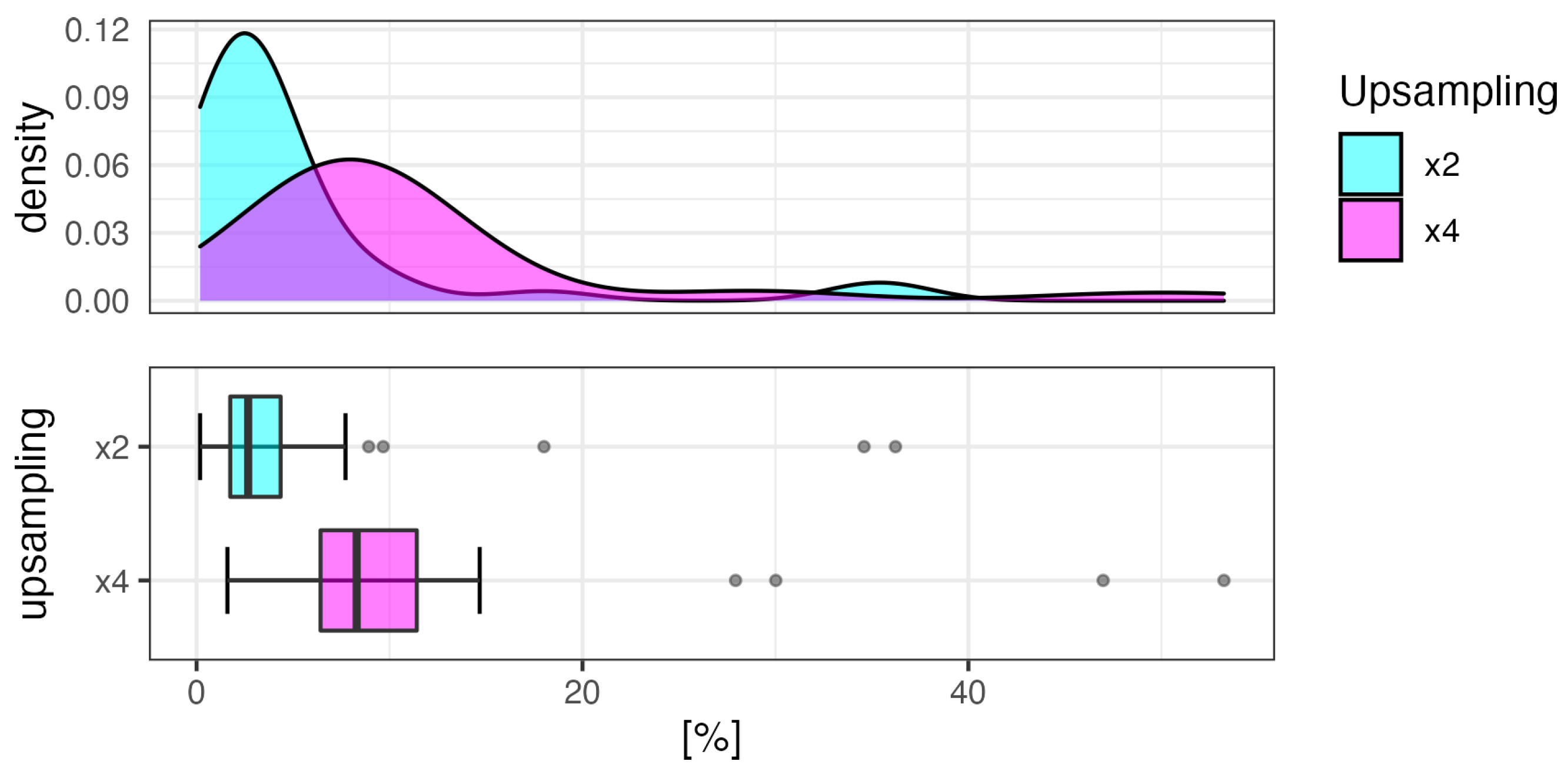
• Upsampling resistant: Granularity changes should be insignificant when the DEM is upsampled (pixel size is made smaller).

The first requirement aims at making the method fully automatic. The second requirement increases the impact of the most prominent terrain features on the granularity value. The third requirement ensures that going to a smaller pixel size by resampling does not alter the granularity, since no landforms are added or removed. A similar requirement for DEM downsampling is not sensible, since transition to the coarser resolution will inevitably destroy small terrain features.

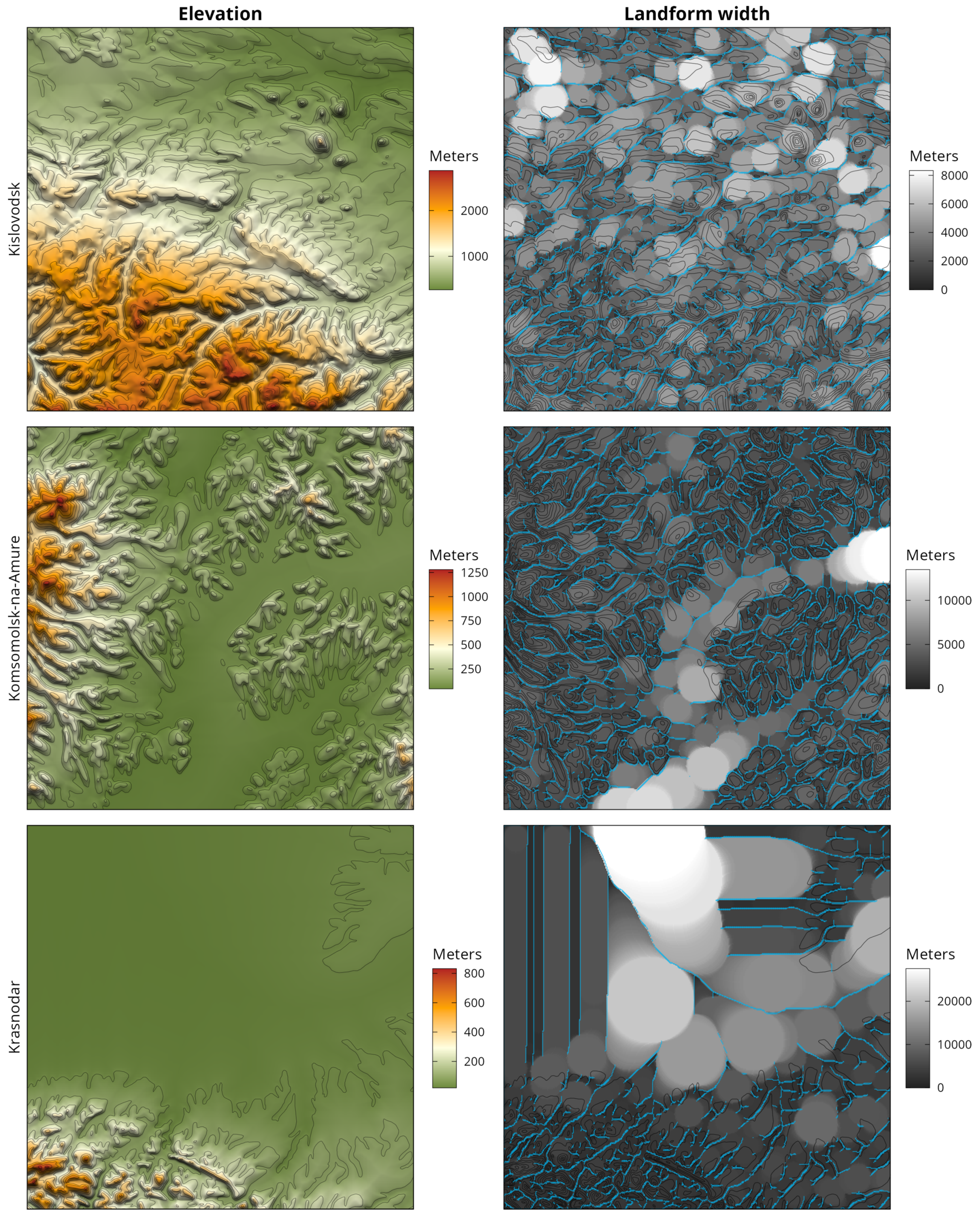
3.2. Landform width Measure

While it is possible to derive the boundaries of landforms using segmentation or some other object-based image analysis technique, such methods require learning or parameterization, which will make the approach less universal. Since the goal was actually not to derive the exact boundaries, but rather to estimate the size of a landform at each DEM pixel, the mediated measure called landform width was developed. It is defined in the following way:

The landform width at each location is the diameter of the largest circle that covers the location and is inscribed in a landform boundary.

A circle-based approach was previously introduced by Samsonov et al. [45] to estimate the width of the space between elevation contours and to reveal wide areas where supplementary contours are needed. The application of this approach in the estimation of the landform width is illustrated in Figure 1. In our explanations, the original term “region” used to define the space between contours is replaced with the term “landform”. Having this, landform width $W\left(p\right)$ at point p located inside landform $l_i$ is defined as the diameter of the largest circle c that contains p and is entirely located within $l_i$:

$$W\left(p\right)=\underset{p\in c\subseteq l_i}{max}d\left(c\right),$$

where d is the diameter of a circle. This largest circle $c=\widehat{C}$ is called a dominant circle for the point p, and the center of this circle (named $p^{\prime }$) is called a dominant circle-reachable neighbor of point p. Figure 1a illustrates the circle-based definition of the landform width. For the clarity of illustration, it shows only a limited number of example points p and $p^{\prime }$ and the corresponding dominant circles.

The continuous field of landform widths is computed by a raster-based approach. First, for each DEM cell, the Euclidean distance to the closest point on a landform boundary is calculated and stored (Figure 1b). Next, an output raster field with the same spatial resolution and coverage is allocated and initialized with zero values. Now, the doubled value of each cell of the distance raster is propagated to the output cells that are covered by the circle neighborhood of the corresponding size (Figure 1c). The resulting value is determined by the following rule: if a pixel is empty or has a value smaller than the doubled value of the distance raster, then its value is replaced with the doubled value of the distance raster; otherwise, it remains unchanged. This is illustrated in Figure 1c, where pixels of the lower left part of circle C are overridden by circle B, which has a larger radius [45]. To speed up the computations, a priority queue was organized where the cells with larger Euclidean distances are processed first.

Having elaborated the method of landform width computation, the next step is to formalize the extraction of the boundaries that would subdivide the DEM into landforms. Since the calculation of the Euclidean distance seeks the closest point along the landform boundary, it is possible not to search for linear boundaries, but approximate them with a limited number of surface-specific points, which are supposed to be located along the boundaries. The drainage points can be used for this purpose, since they are located along the boundaries of positive landforms and are distinctive surface-specific points. Ridges and other types of surface-specific locations can be quite fuzzy if the terrain is not rugged and therefore are unreliable in the approximation of the landform boundaries.

Drainage lines are traditionally extracted by thresholding the flow accumulation (catchment area) raster derived from the D8 flow direction model [46]. However, the hydrological approach is not suitable for our purposes, since the first requirement for the granularity computation method is violated: a value of minimum flow accumulation is needed as a parameter. Hopefully, a connected network of drainage lines is not needed for our purposes, and it is sufficient to have just a set of points located along the drainage lines. This relaxation opens the possibility to use a purely morphometric approach to extract the drainage pixels from a DEM. In particular, a computational scheme based on a $2\times 2$ moving window devised by Band [19] was found to be suitable. In this method, the window is centered by its northwest cell, and the pixel having the largest elevation is marked. After the whole raster is processed with such a window, all the unmarked pixels represent the drainage pixels.

An example of landform width estimation based on drainage pixels is presented in Figure 2a. Drainage pixels are colored in blue. Red dots are the sample locations selected manually to illustrate the circle-based approach. Black circles are the dominant circles calculated for the sample locations. It can be seen that each dominant circle is not necessarily centered at the covered location. While the methodology of the derivation of drainage pixels misses some minor ravines and the resulting set of pixels is not connected, it can be clearly seen that it provides a fairly dense set of characteristic points to approximate the boundaries of positive landforms. The resulting landform width surface is shown in Figure 2b. Supplementary surfaces represented in Figure 2c,d are explained in the following paragraph dedicated to the granularity calculation.

3.3. Granularity Calculation

After the landform width is estimated at each pixel of the DEM, it should be aggregated to obtain one numerical value that characterizes the granularity of the DEM. While it is possible to evaluate granularity just by calculating the mean or median value of the landform width, the resulting value can be biased if the DEM covers morphologically different areas or if the DEM is noisy.

A typical example of the first situation is the case of mapping the mountain foothills: a highly rugged terrain with a dense pattern of small landforms in one part of a map adjoins a flat area where a few landforms can be recognized. A simple average over the area will bias the granularity towards a larger landform width, reducing its potential to consider small landforms. In contrast, noisy DEMs usually contain many small but insignificant artificial “landforms”, which will bias the granularity towards a smaller landform width.

One can note that in both cases, the landforms that bias the resulting granularity have small vertical dimensions. Therefore, if removal of such a bias is desirable, the granularity G must be calculated as a weighted mean of the landform width, where landform height H is used as a weight at each pixel p:

$$G=\frac{{\displaystyle {\sum }_p}W\left(p\right)H\left(p\right)}{{\displaystyle {\sum }_p}H\left(p\right)}.$$

The calculation of H requires the base surface of a “zero” level $Z_0$ from which the height of a landform can be estimated in the vertical direction up to the real surface elevation Z. Since in our case the landforms are positive, such a surface can be reconstructed from the elevations of drainage pixels. The interpolation method for this purpose should be local, i.e., using only the elevations of drainage pixels that limit the current landform. TIN-based interpolation satisfies this property and therefore was applied in the current paper.

The difference $Z\left(q\right)-Z_0\left(q\right)$ is the relative elevation of point q above the base level of a landform. This variable is shown in Figure 2c. The resulting value of landform height can be estimated by finding the maximum difference between the elevation and base surface inside each dominant circle:

$$H\left(p\right)=\underset{q\in \widehat{C}\ni p}{max}\left[Z\left(q\right)-Z_0\left(q\right)\right]$$

This value is propagated to all pixels that are covered by the dominant circle, which reflects their equally important contribution to forming a landform. The resulting landform height surface is represented in Figure 2d. Using such a surface as a weight in averaging the landform width allows satisfying the second requirement of the granularity method: responsiveness to the landform height. Both the height and width variables are calculated at the same time to reduce the need for duplicated propagation.

The general workflow of granularity calculation, which summarizes the developed method, is represented in Figure 3.

Since the quality of cartographic representation is usually assessed in map image units (mm, cm, or in), it is convenient to differentiate between absolute granularity, which is expressed in DEM coordinate system units, and relative granularity, which is expressed in map image units. For example, if the DEM has an absolute granularity of 1500 m, then its relative granularities in 1:200,000 and 1:500,000 scales will be 7.5 mm and 3 mm respectively. For the sake of brevity, we use the term “granularity” for the absolute granularity, while the relative granularity is indicated explicitly in the rest of the paper.

3.4. Resistance to Upsampling

Resolution and granularity are inherently dependent properties of detail. In particular, resolution sets the lower bound of the possible granularity: one pixel is the smallest space available to represent the landform. DEM downsampling (increasing the pixel size) will inevitably affect the granularity, since it is a destructive operation, which coarsens the representation of landforms. The opposite upsampling (decreasing the pixel size) process is non-destructive, but may introduce new subtle details in the surface caused by interpolation. From the perspective of the DEM user, it is undesirable if the granularity estimation method is sensible for these subtle changes. Since it is hardly possible to obtain exactly the same granularity after upsampling, we need to define how exactly the change is measured and what value of change is a significance threshold. For this purposes, we used the change ratio C:

$$C_v=\frac{|v_0-v_1|}{min(v_0,v_1)}\times 100\%,$$

where $v_0$ and $v_1$ are the values of the variable v before and after transformation. The influence of upsampling on granularity was considered to be insignificant if the value of $C_v$ for granularity is at least an order of magnitude (10 times) smaller then the value of $C_v$ for raster resolution. For example, if the pixel size of a DEM is reduced from $R_0=100$ m to $R_1=50$ m ($C_R=100\%$) and the DEM granularity is $G_0=500$ m, then its resulting value $G_1$ must be in the 455–550 m range for $C_G\le 10\%$. This property can be investigated easily by upsampling the DEM and comparing the change ratios for resolution and granularity.

4. Implementation and Data Processing

4.1. Implementation

The developed method was implemented as a free and open-source raster-space processing plugin for QGIS 3.x (https://github.com/tsamsonov/raster-space, accessed 22 February 2022). The computationally intensive part of the processing dedicated to landform width estimation was programmed in the C++ language and linked as compiled Python module. The remaining steps of granularity assessment were completed in the Python language, using the QGIS, GDAL, SAGA, and Whitebox Python bindings. In particular, the extraction of surface-specific points was achieved by the corresponding SAGA function.

4.2. Data Processing

4.2.1. Generation of Reference DEMs

For the current study, we used a multiresolution topographic database with 3 levels of detail, created from Russian topographic maps of 1:200,000, 1:500,000, and 1:1,000,000 mapping scales (referred to interchangeably as 200, 500, and 1000 LoDs). These maps were compiled in 2008–2010 by The Federal Service for State Registrations, Cadaster and Cartography (Rosreestr) using the generalization of larger-scale maps. Each LoD contains a set of layers representing relief, hydrography, vegetation, transportation, settlements, and other standard elements of topographic maps. In particular, relief is represented by contour lines with specific intervals summarized in

Table 1. Contour intervals, m.

Scale	Plains	Mountains
1:200,000	20	40
1:500,000	50	100
1:1,000,000	50, 100	100, 200

. Since these contour lines are generalized manually by mapmakers to achieve the balanced level of detail, they were used to reconstruct reference digital elevation models suitable for analysis with the developed method and then to learn the optimal granularity. For this, 36 fragments centered on Russian settlements located in different terrain conditions (108 fragments in total) were extracted. Each fragment was clipped by a $100\mathrm{km}\times 100\mathrm{km}$ rectangle and then projected into the Lambert azimuthal equal-area projection with the corresponding center. The map of sample fragments’ locations is represented in Figure 4.

Raster DEMs were reconstructed from the extracted contour lines using the approach developed by Koshel [47]. Since the DEMs were created as data sources for constructing the graphical surface representation, they must have fine resolution, which is capable of representing abrupt changes in the terrain surface such as sharp ridges. Specifically, for printed maps that are worked with from a typical distance of 30 cm, the standard graphical quality of $0.1$ mm must be ensured [48] (which, for example, means using a DEM of 50 m resolution is required for mapping at the 1:500,000 scale). For maps on computer screens, which are viewed from 2–3-times greater distances, a proportionally coarser resolution can be applied. Hence, the DEM resolution was set to be $0.25$ mm at the mapping scale, and pixel sizes for 200, 500, and 1000 LoDs were set to 50 m ($2000\times 2000$ px), 125 m ($800\times 800$ px), and 250 m ($400\times 400$ px) correspondingly.

4.2.2. Experiments

Each reference DEM was processed by granularity estimation, which took 47 s, 7 s, and 3 s on average for the DEMs of 200, 500, and 1000 LoDs. Cartographic representations of the resulting reference DEMs for 1000 LoD, as well as calculated landform width rasters are shown in Appendix A, Figure A1, Figure A2, Figure A3, Figure A4, Figure A5, Figure A6, Figure A7, Figure A8, Figure A9, Figure A10, Figure A11 and Figure A12. A classical combination of contours, hypsometric tints, and hill shading was applied in the DEM visualization. The contour interval was selected the same as on the corresponding topographic maps (Table 1), while hypsometric tints and hill shading were similar for all fragments.

The granularities of the created DEMs were statistically analyzed to reveal the optimal relief representation granularity for a small-scale mapping. In particular, the median values and interquartile ranges of granularity were calculated for each LoD, which allowed summarizing the values into the recommended range. The obtained values were also interpreted in the context of Töpfer’s radical law [49] to quantify the intensity of landform selection through scale changes.

To assess the effectiveness of granularity as an essential level of detail component, the following experiment was conducted. Two fragments of NASADEM [2] having the same spatial extent as the Bodaybo and the Groznyy fragments were extracted. The resolution of extracts was 1″, which corresponds to ≈16.5 m for the Bodaybo fragment and ≈23 m for the Groznyy fragment. Each fragment was reprojected by warping into the Lambert azimuthal equal-area projection with the corresponding center and metric resolution. Reprojected DEMs were then generalized using a combination of structural simplification [40] and feature-preserving smoothing [50] until the granularity of the generalized surface became approximately equal ($\pm 5\%$) to the granularity of the reference DEM created from the topographic map. The simplification was used to reduce the density of the landforms, while smoothing was performed to reduce the noise and smooth discontinuities resulting from the TIN-based interpolation of structural lines. The resolution of the generalized DEMs was set to be 50 m, 125 m, and 250 m, correspondingly. For comparison, the source NASADEM fragments were simply resampled (without generalization) using the cubic interpolation to the same resolution $R=50$ m, 125 m, 250 m and separately to the same granularity G as the reference manually generalized DEMs. Resampled models were compared to the generalized ones to check if the resolution or granularity can be used alone to achieve the desired level of detail and to assess the necessity and positive effects of generalization for that purpose.

Finally, the generalized Bodaybo and Groznyy NASADEM extracts were used to assess the sensitivity of the current granularity implementation to DEM upsampling. For this, generalized DEMs for each LoD were upsampled 2 and 4 times using bicubic interpolation, and the granularities of resulting DEMs were compared to the granularities of the non-altered DEMs with the initial resolution. To ensure that the changes were not dependent on the terrain type, a similar experiment was performed for all reference DEM fragments of the 1000 LoD.

5. Results

5.1. Optimal Granularity

To aggregate the granularity data obtained from the reference DEMs, we calculated the summary statistics for each LoD. The distribution of the granularity values can be assessed from Figure 5. In particular, the global median granularity value (indicated by the thick vertical segment in each boxplot) was 1265 m, 2714 m, and 4510 m for the 200, 500, and 1000 LoDs, respectively. This corresponds to the relative granularity of $6.75$ mm, $5.43$ mm, and $4.51$ mm.

Since our experiment was aimed at finding the optimal DEM granularity, we proceeded with finding the value that is the most representative for all analyzed LoDs. For this purpose, we used the median value of the relative granularity and its interquartile range $\left(Q1–Q3\right)$, which is $5.38\left(4.5–6.9\right)$ mm for all 108 DEM fragments. Seeing that the 5–6 mm interval intersects with the interquartile ranges of all LoDs, we derived the following empirical rule of thumb:

The optimal relative granularity of the digital elevation model for small-scale mapping is 5–6 mm.

The observed decrease in relative granularity towards small scales indicated that the relief representation on a map becomes denser after generalization and scale reduction. This tendency characterizes the intensity of landform selection and can be related to Töpfer’s radical law of cartographic generalization. The law states that when the scale is decreased two times, the number of objects generally decreases by $\sqrt{2}$ times [49]. Having that the number of objects is inversely related to the area and the area of the circular object is $\pi r^2$, where $r=W/2$, we can calculate for a $200\to 500$ ($2.5$-times) reduction: $\frac{2^2}{\pi 5.{43}^2}/\frac{2^2}{\pi 6.{75}^2}={\left(\frac{6.75}{5.43}\right)}^2\approx 1.55\approx \sqrt{2.39}$ and similarly, for a $500\to 1000$ (2-times) reduction: ${\left(\frac{5.43}{4.51}\right)}^2\approx 1.45\approx \sqrt{2.10}$.

Our calculations show that the reduction in detail is non-linear: $200\to 500$ is more conservative (kept more features than expected), while $500\to 1000$ is more selective (kept less features than expected). Such a non-linearity in selection is quite natural for topographic maps, since each mapping scale serves best for solving the specific set of problems, and therefore, the intensity of generalization varies between map scales to facilitate the problem solving. The complete $200\to 1000$ (5-times) LoD change is characterized by a ${\left(\frac{6.75}{4.51}\right)}^2\approx 2.24\approx \sqrt{5.01}$-times reduction in the number of landforms, which fits perfectly the expected $\sqrt{5}$ value.

This observation can be summarized in the following important result:

Landform selection intensity during relief generalization on topographic maps follows Töpfer’s radical law.

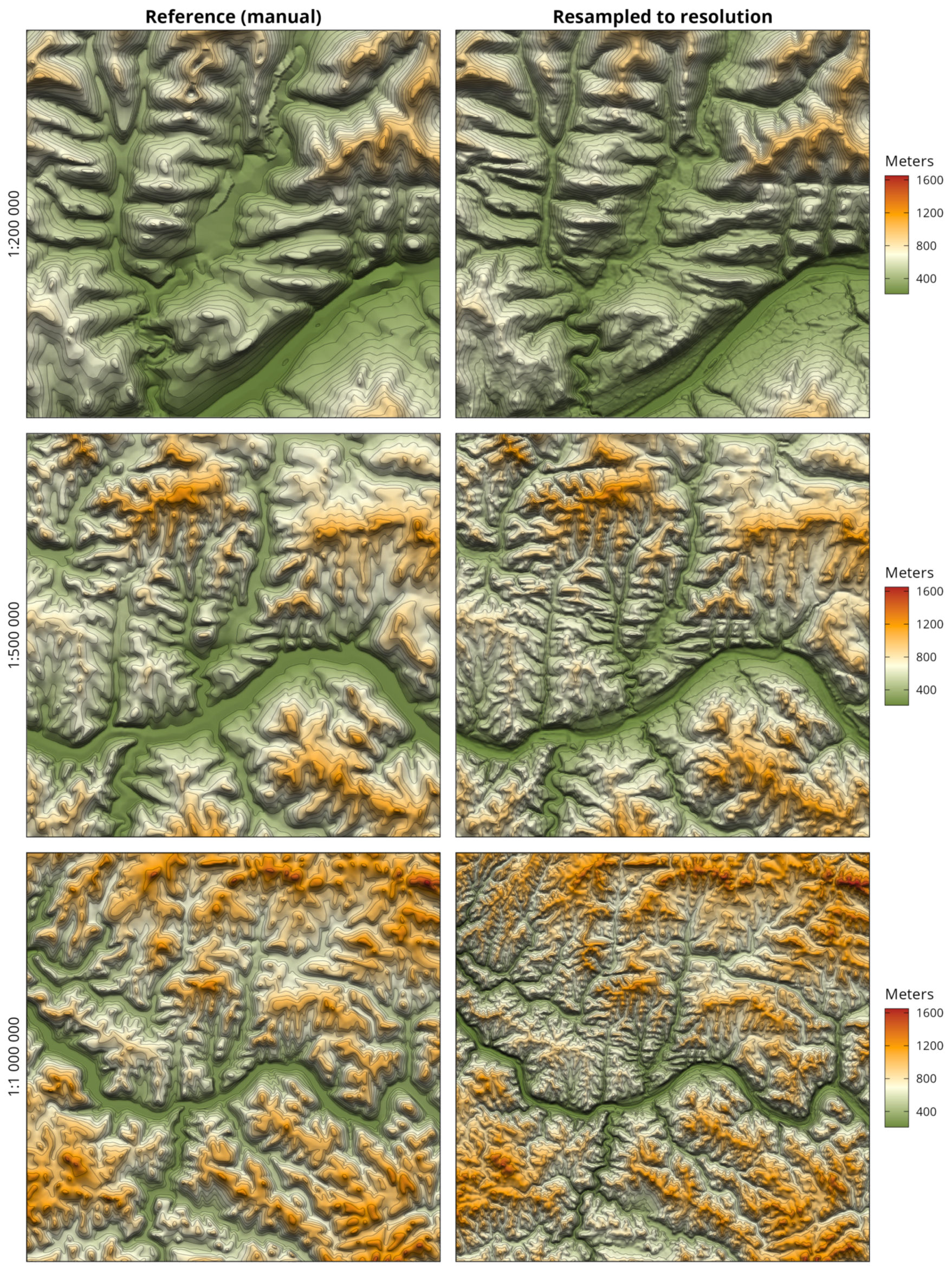
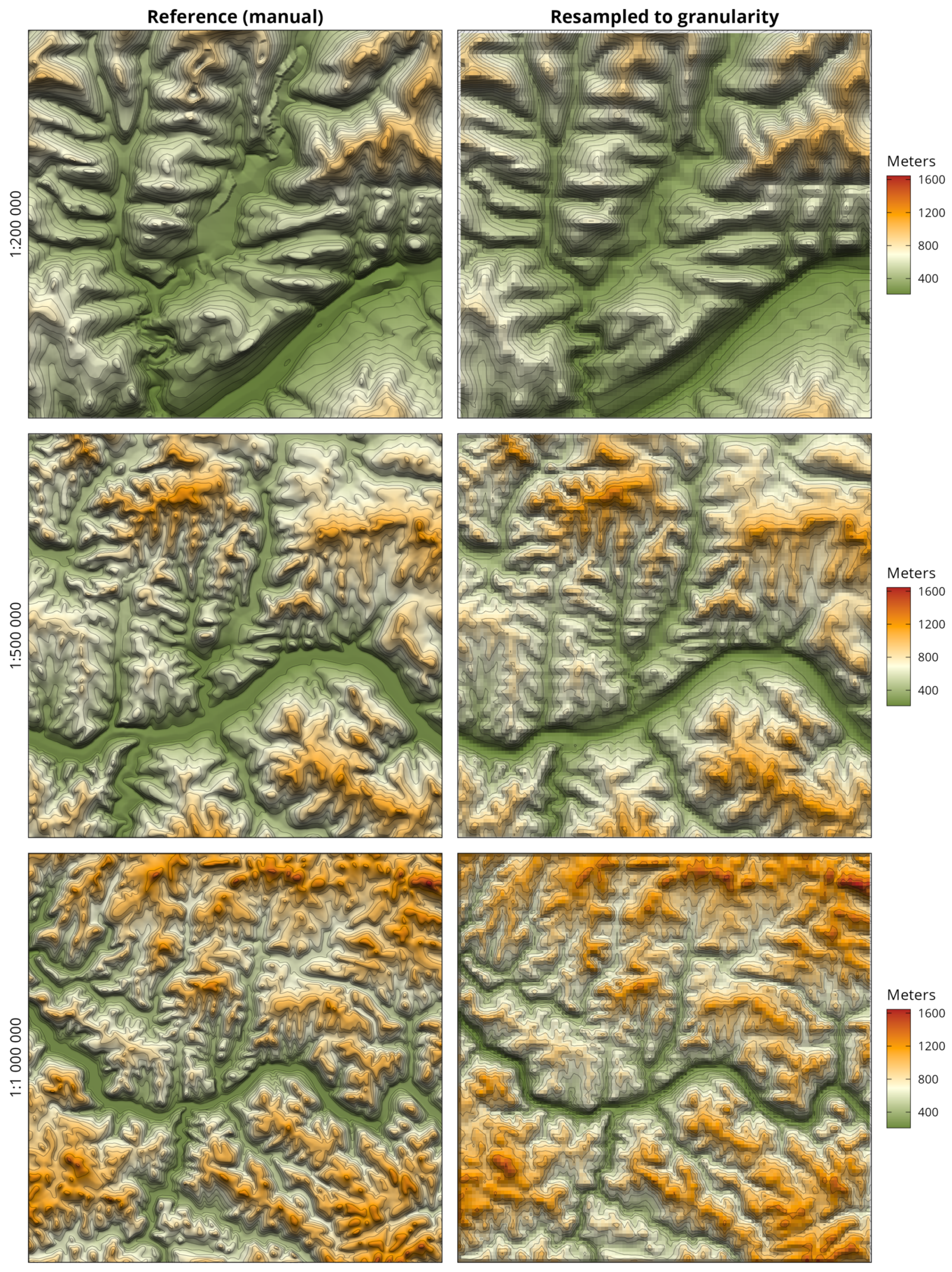
5.2. DEM Generalization and Optimal Level of Detail

Granularity values for the manual (reference), generalized, and resampled DEMs derived in the second experiment are presented in

Table 2. DEM granularity.

			Granularity, m
Fragment	LoD	Resolution	Reference	Generalization	Resampling to G	Resampling to R
Bodaybo	200	50	1595	1611	1606	1073
	500	125	2282	2275	2278	1407
	1000	250	3678	3780	3864	1750
Groznyy	200	50	1392	1436	1339	501
	500	125	2992	2966	3109	927
	1000	250	4510	4448	4689	1662

.

The Bodaybo fragment covers mountainous areas with a homogeneous terrain structure. The generalization of such a DEM is a straightforward process, since each landform is characterized by a similar size and morphology. The comparison of the generalized NASADEM extracts and the corresponding reference DEMs is represented in Figure 6. Supplementary landform width rasters for the same DEMs are shown in Figure 7. We see that the automated generalization is slightly smoother than manual, but the differences in the overall level of detail of both DEMs are visually insignificant, which showed that the granularity measure is effective as a constraint for DEM generalization. This conclusion can be supplemented by analyzing the landform width rasters represented in Figure 7, which also are characterized by a similar pattern of dominant circles. Figure 8 presents the resampling of the Bodaybo NASADEM fragment to the same resolution R as the reference DEMs. It is clear that in all cases, the amount of detail in resampled NASADEM is higher, and the difference becomes more significant at coarser resolutions, which is asserted by smaller granularity values in resampling to the R column of Table 2. Figure 9 presents the resampling of NASADEM to the same granularity G as the reference DEMs. The resulting raster resolutions are $200,425,850$ m for the 200, 500, and 1000, LoDs respectively. In this case, the size of the represented landforms is quite similar in the resampled and reference DEMs, which means that the granularity performes its function effectively. However, the graphical quality of the representation is low due to the excessively large pixel size.

The Groznyy fragment covers a heterogeneous combination of flat, foothill, and mountainous terrain, which makes it quite difficult to generalize. In addition, the source NASADEM fragment covering this area is noisy. The generalized NASADEM extracted for this fragment can be compared to the reference manual DEMs in Figure 10. Supplementary landform width rasters are represented in Figure 11. As expected, the generalized examples contain a large number of small landforms in noisy areas. However, since these landforms have a small height, their weight in the estimated granularity value is negligible. Hence, the automatically generalized DEMs are only slightly smoother than the manual ones, and the both have a visually similar level of detail. Figure 12 presents the resampling of the Groznyy NASADEM extract to the same resolution R as the reference DEMs. Figure 13 shows the NASADEM resampled to the same granularity G as the reference DEMs. The resulting raster resolutions were $225,425,575$ m for the 200, 500, and 1000 LoDs, respectively. One can note that for the 1000 LoD, the resolution (575 m) is significantly higher than in the case of the Bodaybo fragment (850 m), which means that due to the morphological properties of the terrain, downsampling changes the DEM granularity more intensively. Visual analysis of the results brings the same conclusions as in the Bodaybo case: resampling to the same (high) resolution results in an excessive amount of detail, while resampling to the same granularity limits the size of the represented landforms in an optimal way, but the coarse DEM resolution is insufficient for high-quality relief presentation.

To supplement the visual comparisons of the differences in detail between the experimental DEMs, a statistical assessment of landform width rasters was performed. Figure 14 shows the distributions of the landform width for the Bodaybo (a) and Groznyy (b) fragments. The analysis of these figures reveals that the results constrained by granularity (generalization and resampling to G) are considerably more similar to the manually generalized reference DEM than resampling to the same resolution R. This is reflected not only in central tendency of the landform width, but also in the shape of its distribution, which can be assessed from the density and box plots. A significant number of large outliers can be seen in the boxplots for both fragments. These outliers indicate a heterogeneous nature of the terrain where the landforms are predominantly small, but a noticeable number of large landforms are located in some places. The more complex Groznyy fragment exhibits this property more brightly.

Statistical testing of the differences in the mean and variance between distributions using the Student (Welch) and Fisher tests showed highly significant ($p<0.001$) differences in any combination of distributions, which was mainly due to the high power of the statistic: the number of DEM pixels for the 200, 500, and 1000 LoDs was about 4,000,000, 600,000, and 150,000, respectively. Hence, the integral assessment of the differences in distributions was performed using the Kolmogorov–Smirnov D statistic, the values of which are represented in

Table 3. Kolmogorov–Smirnov D statistic for width distributions with manually generalized DEMs as a source for the reference width distribution.

		D
Fragment	LoD	Resampling to R	Resampling to G	Generalization
Bodaybo	200	0.3493	0.0430	0.0000
	500	0.4650	0.1377	0.0000
	1000	0.7090	0.1654	0.0141
Groznyy	200	0.5263	0.3015	0.1820
	500	0.7730	0.1638	0.0278
	1000	0.7455	0.1976	0.0565

. The results are also highly significant ($p<0.001$), which means that the distributions differ from each other. However, now we see clearly that DEM generalization outperformed resampling constrained by G in terms of the proximity to the manual reference. In the worst case of the 200 LoD for the Groznyy fragment, the generalized DEM is $0.3015/0.1820\approx 1.66$-times closer to the reference DEM, while for the best cases of the Bodaybo 200 and 500 fragments $D<0.0001$ for the generalized DEM, while resampling to G is larger than $0.01$ in both cases. Resampling to R brought the worst statistics overall, as expected.

The results obtained in this part of the experiment helped us formulate the following inference:

The optimal level of detail in small-scale cartographic relief presentation requires a combination of DEM generalization constrained by granularity and a fine resolution of the generalized DEM which facilitates the high quality of visualization. DEM resampling alone is not effective for this purpose.

5.3. DEM Upsampling and Resistance of Granularity

The DEM resolution change ratios for $\times 2$ and $\times 4$ upsamplings (on the example of the 200 LoD) are $\frac{|50-25|}{min(50,25)}\times 100\%=100\%$ and $\frac{|50-12.5|}{min(50,12.5)}\times 100\%=300\%$, correspondingly. Following the “order of magnitude smaller” rule established in Section 3.4, the granularity change ratios are considered insignificant if they are smaller than $10\%$ and $30\%$, respectively.

The granularities of the upsampled generalized Bodaybo and Groznyy NASADEM extracts are presented in

Table 4. Resistance of granularity to DEM upsampling.

			Bodaybo		Groznyy
LoD	Upsampling	Resolution, m	Granularity, m	Change, %	Granularity, m	Change, %
200	×4	12.50	1588	1.45	1390	3.31
200	×2	25.00	1597	0.88	1408	1.99
200	×1	50.00	1611	0.00	1436	0.00
500	×4	31.25	2147	5.96	2693	10.14
500	×2	62.50	2208	3.03	2750	7.85
500	×1	125.00	2275	0.00	2966	0.00
1000	×4	62.50	3611	4.68	3887	14.43
1000	×2	125.00	3681	2.69	4144	7.34
1000	×1	250.00	3780	0.00	4448	0.00

. The worst granularity change ratios for 2- and 4-times upsampling are $7.85\%$ and $14.43\%$, respectively, which are both insignificant according to the considerations above.

The distributions of the granularity change ratios of all 1000 LoD reference DEMs for $\times 2$ and $\times 4$ upsampling are plotted in Figure 15. The median values and interquartile ranges are $2.7\left(1.7–4.4\right)$% and $8.3\left(6.4–11.4\right)$%, correspondingly. This means that in general, the granularity change ratio is insignificant, as in the previous experiment. However, there are several outliers. For $\times 2$ upsampling, such fragments are Bratsk ($18.0\%$ change), Petropavlovsk-Kamchatskiy ($36.2\%$ change), and Vladivostok ($34.6\%$ change). For $\times 4$ upsampling, these fragments are Bratsk ($27.9\%$ change), Petropavlovsk-Kamchatskiy ($47.0\%$ change), Ukhta ($30.0\%$ change), and Vladivostok ($53.2\%$ change). Our observations show that these changes occur when the DEM contains large portions of flat areas (plains, plateaus, or water bodies). Over these areas, small variations in elevation due to resampling could be the same order of magnitude as the variations existing in the source DEM. Hence, upsampling may lead to the appearance of new surface-specific points that decrease the landform width in these areas up to 2–3 times. Such sensitivity should be overcome by more robust future implementations of surface-specific point extraction.

6. Discussion

The proposed approach to DEM granularity estimation bears some important properties, which must be taken into account for its practical application. Some of these properties follow from the methodological design and implementation of the method, while others were inferred from the experimental results obtained in the current research. The most important ones can be summarized as follows.

• Granularity was developed and evaluated as a property of the DEM for mapping purposes. Hence, it helps to ensure that cartographic relief presentation has the desired level of detail. While granularity can be potentially valuable for DEM analysis, such an application is out of the scope of the current paper and requires a separate investigation;
• Granularity is not equivalent to the level of detail and must be used in conjunction with other LoD properties to characterize the DEM comprehensively. The precision, accuracy, and vertical resolution of the elevation data also affect the LoD of the DEM. However, it is the horizontal DEM resolution that is the crucially important granularity counterpart in LoD estimation for small-scale mapping purposes. In particular, if the horizontal resolution is too coarse, the resulting image will not be sharp enough to achieve the desired image quality. The influence of other enlisted properties on the overall LoD of the DEM is more important for analytical and large-/middle-scale mapping purposes and should be investigated in a specially dedicated research work;
• Granularity characterizes the typical size of landforms represented on the DEM surface, but says nothing about their morphology. At the same time, different DEM generalization methods result in surfaces that tend to be smooth or crude, which may distort the initial character of the landforms. Gaussian filtering and structural-TIN-based simplification are examples of such contrasting approaches. To evaluate how realistic the landform representation is after generalization, advanced morphological techniques must be applied in addition to the estimation of granularity;
• The proposed approach to calculate the DEM granularity is based on the landform width measure, which is defined in terms of the distance between surface-specific points. Currently, only drainage pixels are used for this purpose. However, any type of surface-specific point can be incorporated in the calculation of the landform width. In particular, if some objective algorithm for delineating landform boundaries will be developed, the resulting lines or polygons can be used instead of the surface-specific points in the granularity assessment without any need to change the methodology;
• Drainage pixels that are extracted from the surface can be quite sporadic and accidental at places. In this case, some additional filtering (e.g., removing of the single outlier pixels) can improve the quality of landform width assessment and reduce its susceptibility to noise. Currently, no such processing has been applied to demonstrate the effectiveness of the developed method in the wild. We also revealed that for DEMs representing the flat relief, the simple morphometric approach to drainage pixel extraction can be sensible for DEM upsampling. Therefore, its robustness must be improved in future investigations;
• Evaluations of typical DEM granularity are based in this paper on reference DEMs reconstructed from manually drawn topographic maps with a horizontal resolution of $0.25$ mm at the mapping scale. It is possible to achieve the same granularity with a much coarser resolution. However, our experiments showed convincingly that the optimal level of detail for high-quality small-scale cartographic relief presentation requires a fine resolution of the DEM in addition to a reasonable DEM granularity.

Following these considerations should facilitate more meaningful use and improvement of the developed method.

7. Conclusions

Granularity characterizes the typical size of the landforms represented on the DEM surface. The elaboration of this concept was motivated by the fact that the existing DEM quality measures such as resolution and accuracy are not capable of characterizing the detail of the DEM for mapping purposes. Consequently, up to date, it has been problematic to answer if the DEM is generalized properly to fit the scale of visualization.

The computation of granularity was implemented through a simple, but effective proxy measure called the landform width, which is based on circles inscribed in a set of surface-specific points. The fact that the landform width does not require the delineation of exact landform boundaries (which are quite disputable) makes it easy to implement and use. It was also shown that the whole process of granularity estimation can be performed without any parameters, which is a very convenient property from the practical point of view.

Experimental work conducted on multiple examples of reference DEMs reconstructed from manually generalized topographic maps allowed the derivation of the rule of thumb for selecting the optimal relative granularity for small-scale mapping, which is approximately 5–6 mm at the scale of visualization. Since this is a median value, the complexity of the terrain may require the adjustment of this property. Another important practical output of the conducted research is the experimental evidence that the landform selection during relief generalization follows the Töpfer’s radical law.

Two case studies covering homogeneous and heterogeneous terrains showed that granularity works effectively as a constraining measure for DEM generalization, while resampling alone is not sufficient for that purpose. In both cases, the combination of the resolution and granularity constraints resulted in a similar level of detail of manually and automatically generalized DEMs. A classical combination of contours, hypsometric tints, and hill shading was used as a relief presentation method throughout the study.

In future investigations, it would be desirable to perform a user study to additionally assess the robustness of granularity as a measure characterizing the DEM’s level of detail for mapping purposes. The analytical applications of granularity in terrain analysis and geomorphometry are also potentially valuable directions of future research.

References

1. Yamazaki, D.; Ikeshima, D.; Tawatari, R.; Yamaguchi, T.; O’Loughlin, F.; Neal, J.; Sampson, C.; Kanae, S.; Bates, P. A high-accuracy map of global terrain elevations: Accurate Global Terrain Elevation map. Geophys. Res. Lett. 2017, 44, 5844–5853. [Google Scholar] [CrossRef] [Green Version]
2. NASADEM Merged DEM Global 1 Arc Second V001. 2020. Available online: https://cmr.earthdata.nasa.gov/search/concepts/C1546314043-LPDAACECS.html (accessed on 13 February 2022).
3. Guillaume, A.; Leempoel, K.; Rochat, E.; Rogivue, A.; Kasser, M.; Gugerli, F.; Parisod, C.; Joost, S. Multiscale Very High Resolution Topographic Models in Alpine Ecology: Pros and Cons of Airborne LiDAR and Drone-Based Stereo-Photogrammetry Technologies. Remote Sens. 2021, 13, 1588. [Google Scholar] [CrossRef]
4. Imhof, E. Cartographic Relief Presentation; Walter der Gruyter: Berlin, Germany, 1982. [Google Scholar]
5. Ruas, A.; Bianchin, A. Echelle et Niveau de Detail; Generalisation et Representation Miltiple, Hermes Lavoisier: Paris, France, 2002; pp. 25–44. [Google Scholar]
6. Zarutskaya, I. Methods of Representing Relief on Hypsometric Maps; Publishing House of Geodesic Literature: Moscow, Russia, 1958. [Google Scholar]
7. Military Topographic Service. Guide to Cartographic and Cartographic Works. Part 2. Drafting and Preparation for Publication of 1:200,000 and 1:500,000 Topographic Maps; Editorial and Publishing Department of Military Topographic Service: Moscow, Russia, 1980. [Google Scholar]
8. Swiss Society of Cartography. Cartographic Generalization: Topographic Maps, 2nd ed.; Swiss Society of Cartography: Zürich, Switzerland, 1987. [Google Scholar]
9. Polidori, L.; El Hage, M. Digital Elevation Model Quality Assessment Methods: A Critical Review. Remote Sens. 2020, 12, 3522. [Google Scholar] [CrossRef]
10. Wechsler, S. Perceptions by Digital Elevation Model Users of DEM Uncertainty. URISA J. 2003, 15, 1–10. [Google Scholar]
11. Florinsky, I. Accuracy of local topographic variables derived from digital elevation models. Int. J. Geogr. Inf. Sci. 1998, 12, 47–62. [Google Scholar] [CrossRef]
12. Höhle, J.; Höhle, M. Accuracy assessment of digital elevation models by means of robust statistical methods. ISPRS J. Photogramm. Remote Sens. 2009, 64, 398–406. [Google Scholar] [CrossRef] [Green Version]
13. Mesa-Mingorance, J.; Ariza-López, F. Accuracy Assessment of Digital Elevation Models (DEMs): A Critical Review of Practices of the Past Three Decades. Remote Sens. 2020, 12, 2630. [Google Scholar] [CrossRef]
14. Zhou, Q.; Liu, X.; Sun, Y. Terrain complexity and uncertainties in grid-based digital terrain analysis. Int. J. Geogr. Inf. Sci. 2006, 20, 1137–1147. [Google Scholar] [CrossRef]
15. Erdogan, S. Modelling the spatial distribution of DEM error with geographically weighted regression: An experimental study. Comput. Geosci. 2010, 36, 34–43. [Google Scholar] [CrossRef]
16. Guth, P.L.; Van Niekerk, A.; Grohmann, C.H.; Muller, J.P.; Hawker, L.; Florinsky, I.V.; Gesch, D.; Reuter, H.I.; Herrera-Cruz, V.; Riazanoff, S.; et al. Digital Elevation Models: Terminology and Definitions. Remote Sens. 2021, 13, 3581. [Google Scholar] [CrossRef]
17. Podobnikar, T. Methods for visual quality assessment of a digital terrain model. Surv. Perspect. Integr. Environ. Soc. 2008, 1, 1–11. [Google Scholar]
18. Peucker, T.; Douglas, D. Detection of Surface-Specific Points by Local Parallel Processing of Discrete Terrain Elevation Data. Comput. Graph. Image Process. 1975, 4, 375–387. [Google Scholar] [CrossRef]
19. Band, L. Topographic Partition of Watersheds with Digital Elevation Models. Water Resour. Res. 1986, 20, 15–24. [Google Scholar] [CrossRef]
20. O’Callaghan, J.; Mark, D. The extraction of drainage networks from digital elevation data. Comput. Vis. Graph. Image Process. 1984, 28, 323–344. [Google Scholar] [CrossRef]
21. Jenson, S.; Domingue, J. Extracting Topographic Structure from Digital Elevation Data for Geographic Information System Analysis. Photogramm. Eng. Remote Sens. 1988, 54, 1593–1600. [Google Scholar]
22. Iwahashi, J.; Pike, R. Automated classifications of topography from DEMs by an unsupervised nested-means algorithm and a three-part geometric signature. Geomorphology 2007, 86, 409–440. [Google Scholar] [CrossRef]
23. Schmidt, J.; Hewitt, A. Fuzzy land element classification from DTMs based on geometry and terrain position. Geoderma 2004, 121, 243–256. [Google Scholar] [CrossRef]
24. Wood, J. Scale-based Characterization of Digital Elevation Models. In Innovations in GIS; CRC Press: Boca Raton, FL, USA, 1996; Volume 3, pp. 163–175. [Google Scholar]
25. Drăguţ, L.; Blaschke, T. Automated classification of landform elements using object-based image analysis. Geomorphology 2006, 81, 330–344. [Google Scholar] [CrossRef]
26. Romstad, B.; Etzelmüller, B. Mean-curvature watersheds: A simple method for segmentation of a digital elevation model into terrain units. Geomorphology 2012, 139–140, 293–302. [Google Scholar] [CrossRef] [Green Version]
27. Jasiewicz, J.; Stepinski, T. Geomorphons—A pattern recognition approach to classification and mapping of landforms. Geomorphology 2013, 182, 147–156. [Google Scholar] [CrossRef]
28. Guilbert, E.; Gaffuri, J.; Jenny, B. Terrain Generalisation; Abstracting Geographic Information in a Data Rich World; Springer International Publishing: Cham, Switzerland, 2014; pp. 227–258. [Google Scholar] [CrossRef]
29. Loon, J. Cartographic Generalization of Digital Terrain Models. Ph.D. Thesis, The Ohio State University, Columbus, OH, USA, 1977. [Google Scholar]
30. Weibel, R. An Adaptive Methodology for Automated Relief Generalization. In Proceedings of the AutoCarto 8, Baltimore, MD, USA, 29 March–3 April 1987; pp. 42–49. [Google Scholar]
31. Zakšek, K.; Podobnikar, T. An effective DEM generalization with basic GIS operations. In Proceedings of the 8th ICA Workshop on Generalisation and Multiple Representation, La Coruńa, Spain, 9–16 July 2005. [Google Scholar]
32. Pedrini, H. Multiresolution terrain modeling based on triangulated irregular networks. Revista Brasileira de Geociencias 2001, 31, 117–122. [Google Scholar] [CrossRef]
33. Wang, Z.; Li, Q.; Yang, B. Multi-Resolution Representation of Digital Elevation Models With Topographical Features Preservation. Int. Arch. Photogramm. Remote Sens. Spat. Inf. Sci. 2008, 37, 1–7. [Google Scholar]
34. Chen, Y.; Wilson, J.; Zhu, Q.; Zhou, Q. Comparison of drainage-constrained methods for DEM generalization. Comput. Geosci. 2012, 48, 41–49. [Google Scholar] [CrossRef]
35. Zhou, Q.; Chen, Y. Generalization of DEM for terrain analysis using a compound method. ISPRS J. Photogramm. Remote Sens. 2011, 66, 38–45. [Google Scholar] [CrossRef]
36. Jordan, G. Adaptive smoothing of valleys in DEMs using TIN interpolation from ridgeline elevations: An application to morphotectonic aspect analysis. Comput. Geosci. 2007, 33, 573–585. [Google Scholar] [CrossRef]
37. Ai, T.; Li, J. A DEM generalization by minor valley branch detection and grid filling. ISPRS J. Photogramm. Remote Sens. 2010, 65, 198–207. [Google Scholar] [CrossRef]
38. Weibel, R. Models and Experiments for Adaptive Computer-Assisted Terrain Generalization. Cartogr. Geogr. Inf. Sci. 1992, 19, 133–153. [Google Scholar] [CrossRef]
39. Leonowicz, A.; Jenny, B.; Hurni, L. Automatic generation of hypsometric layers for small-scale maps. Comput. Geosci. 2009, 35, 2074–2083. [Google Scholar] [CrossRef] [Green Version]
40. Samsonov, T. Multiscale Hypsometric Mapping. In Lecture Notes in Geoinformation and Cartography; Springer: Berlin/Heidelberg, Germany, 2011; Volume 1, pp. 497–520. [Google Scholar]
41. Raposo, P. Variable DEM generalization using local entropy for terrain representation through scale. Int. J. Cartogr. 2020, 6, 99–120. [Google Scholar] [CrossRef]
42. Zhang, C.; Pan, M.; Wu, H.; Xu, H. Study on simplification of contour lines preserving topological coherence. Acta Sci. Nat. Univ. Pekin. 2007, 43, 216–222. [Google Scholar]
43. Ai, T. The drainage network extraction from contour lines for contour line generalization. ISPRS J. Photogramm. Remote Sens. 2007, 62, 93–103. [Google Scholar] [CrossRef]
44. Chen, Y.; Ma, T.; Chen, X.; Chen, Z.; Yang, C.; Lin, C.; Shan, L. A New DEM Generalization Method Based on Watershed and Tree Structure. PLoS ONE 2016, 11, e0159798. [Google Scholar] [CrossRef] [PubMed]
45. Samsonov, T.; Koshel, S.; Walther, D.; Jenny, B. Automated placement of supplementary contour lines. Int. J. Geogr. Inf. Sci. 2019, 33, 2072–2093. [Google Scholar] [CrossRef]
46. Mark, D. Automated Detection Of Drainage Networks From Digital Elevation Models. Cartogr. Int. J. Geogr. Inf. Geovis. 1984, 21, 168–178. [Google Scholar] [CrossRef]
47. Koshel, S. Algorithm for Topologically Correct Gridding of Contour Data. In Proceedings of the Seventh International Conference on Geographic Information Science (GIScience 2012), Columbus, OH, USA, 18–21 September 2012; pp. 1–5. [Google Scholar] [CrossRef]
48. Kennelly, P.; Patterson, T.; Jenny, B.; Huffman, D.; Marston, B.; Bell, S.; Tait, A. Elevation models for reproducible evaluation of terrain representation. Cartogr. Geogr. Inf. Sci. 2021, 48, 63–77. [Google Scholar] [CrossRef]
49. Töpfer, F.; Pillewizer, W. The Principles of Selection. Cartogr. J. 1966, 3, 10–16. [Google Scholar] [CrossRef]
50. Sun, X.; Rosin, P.; Martin, R.; Langbein, F. Fast and Effective Feature-Preserving Mesh Denoising. IEEE Trans. Vis. Comput. Graph. 2007, 13, 925–938. [Google Scholar] [CrossRef]
Figure 1. Circle-based landform width computation (adopted from [45]): (a) Circle-based definition of the landform width (brighter circles represent larger width). Points p’ are dominant circle-reachable neighbors of example points p. Their circles A, B, C, and D are drawn in white. (b) A scalar field with the distance to the nearest point along the landform boundary. (c) Propagation of the doubled distance to the circle neighborhood of the corresponding size (brighter pixels represent larger circle diameters). Pixel size is 2.5 m.
Remotesensing 14 01270 g001
Figure 2. Preliminary steps of granularity calculation: (a) sample locations and their dominant circles inscribed in a set of drainage pixels; (b) landform width; (c) relative elevation—a difference between the elevation and base surface reconstructed from the triangulation of the drainage pixels; (d) landform height.
Remotesensing 14 01270 g002
Figure 3. General workflow of DEM granularity calculation.
Remotesensing 14 01270 g003
Figure 4. Locations of sample fragments.
Remotesensing 14 01270 g004
Figure 5. Distributions of the granularity for DEMs generated from three levels of detail of the topographic maps: (a) absolute granularity; (b) relative granularity.
Remotesensing 14 01270 g005
Figure 6. Comparison of the reference DEM and the NASADEM extract generalized automatically to the same granularity (Bodaybo fragment, elevation).
Remotesensing 14 01270 g006
Figure 7. Comparison of the reference DEM and the NASADEM extract generalized automatically to the same granularity (Bodaybo fragment, landform width).
Remotesensing 14 01270 g007
Figure 8. Comparison of the reference DEM and the NASADEM extract resampled to the same resolution (Bodaybo fragment, elevation).
Remotesensing 14 01270 g008
Figure 9. Comparison of the reference DEM and the NASADEM extract resampled to the same granularity (Bodaybo fragment, elevation).
Remotesensing 14 01270 g009
Figure 10. Comparison of the reference DEM and the NASADEM extract generalized automatically to the same granularity (Groznyy fragment, elevation).
Remotesensing 14 01270 g010
Figure 11. Comparison of the reference DEM and the NASADEM extract generalized automatically to the same granularity (Groznyy fragment, landform width).
Remotesensing 14 01270 g011
Figure 12. Comparison of the reference DEM and the NASADEM extract resampled to the same resolution (Groznyy fragment, elevation).
Remotesensing 14 01270 g012
Figure 13. Comparison of the reference DEM and NASADEM extract resampled to the same granularity (Groznyy fragment, elevation).
Remotesensing 14 01270 g013
Figure 14. Absolute landform width (weighted by height) for the Bodaybo (a) and Groznyy (b) fragments. Distributions for the reference, generalized, resampled to the same granularity (G), and resolution (R) DEMs are shown by different fill colors.
Remotesensing 14 01270 g014
Figure 15. Granularity change ratio due to upsampling.
Remotesensing 14 01270 g015