
Integration of Sentinel-3 and MODIS Vegetation Indices with ERA-5 Agro-Meteorological Indicators for Operational Crop Yield Forecasting

 , , , , ,
Abstract
:1. Introduction
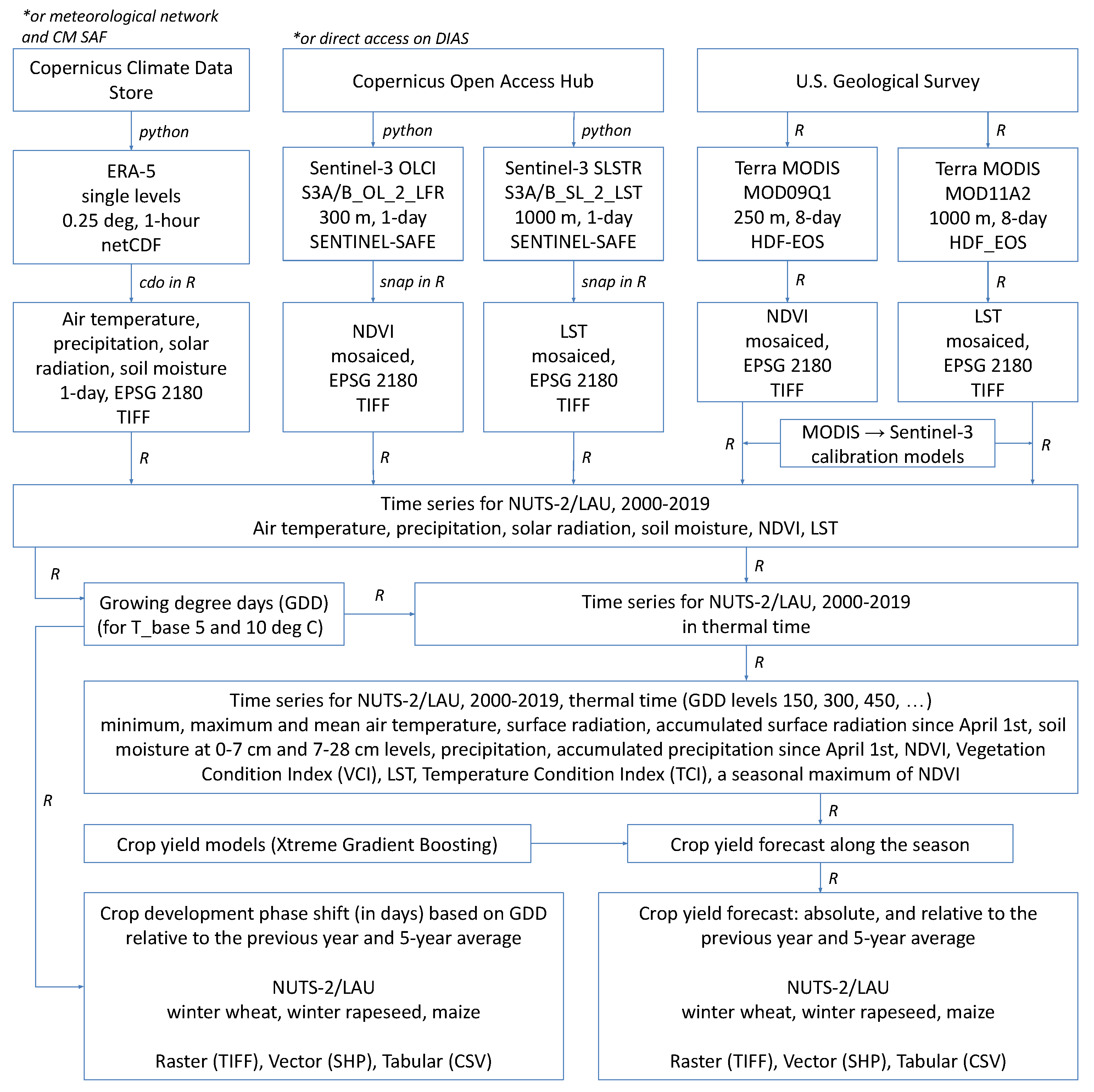
2. Data
2.1. Satellite Data
2.1.1. Sentinel-3 Operational Products
- Land Full Resolution (LFR) product derived from OLCI imagery at a 300-m resolution consisting of Global Vegetation Index (OGVI) and Terrestrial Chlorophyll Index (OTCI) indices accompanied with rectified reflectances at 681 nm (RED) and 865 nm (NIR) channels used in this study to calculate Normalized Difference Vegetation Index (NDVI) using formula:
- Land Surface Temperature (LST) from the SLSTR sensor at a 1-km resolution.
2.1.2. MODIS Products
2.2. Agro-Meteorological Data
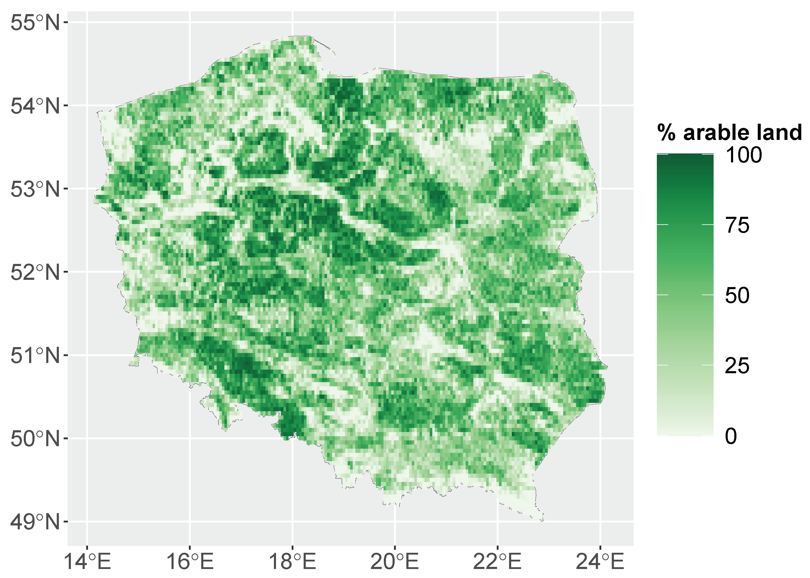
2.3. Crop Mask
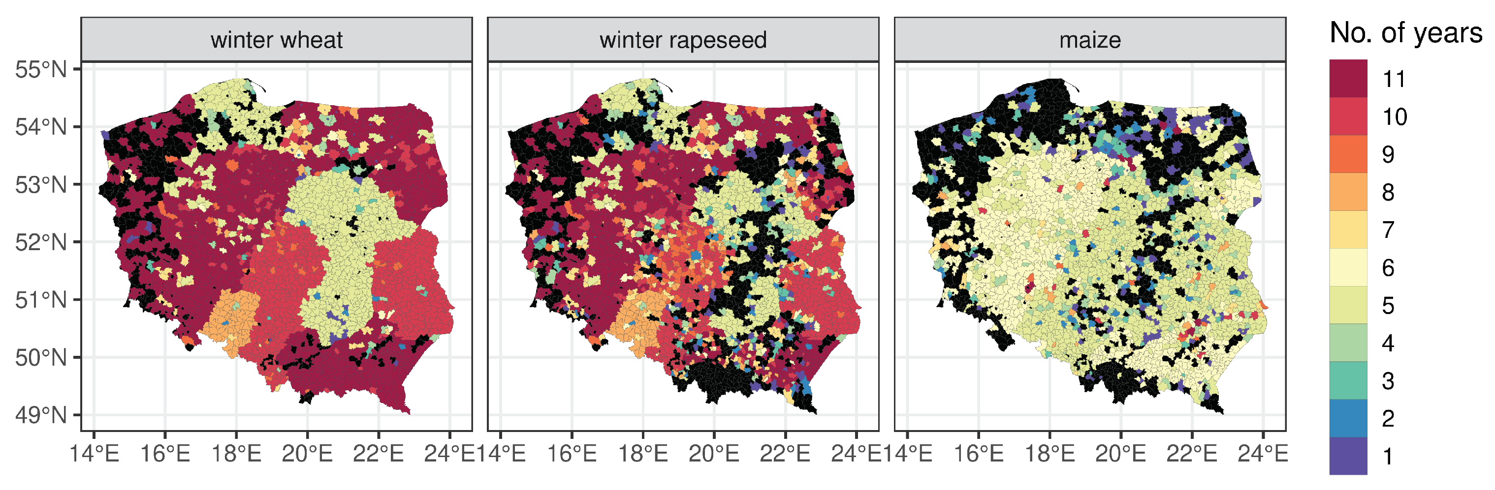
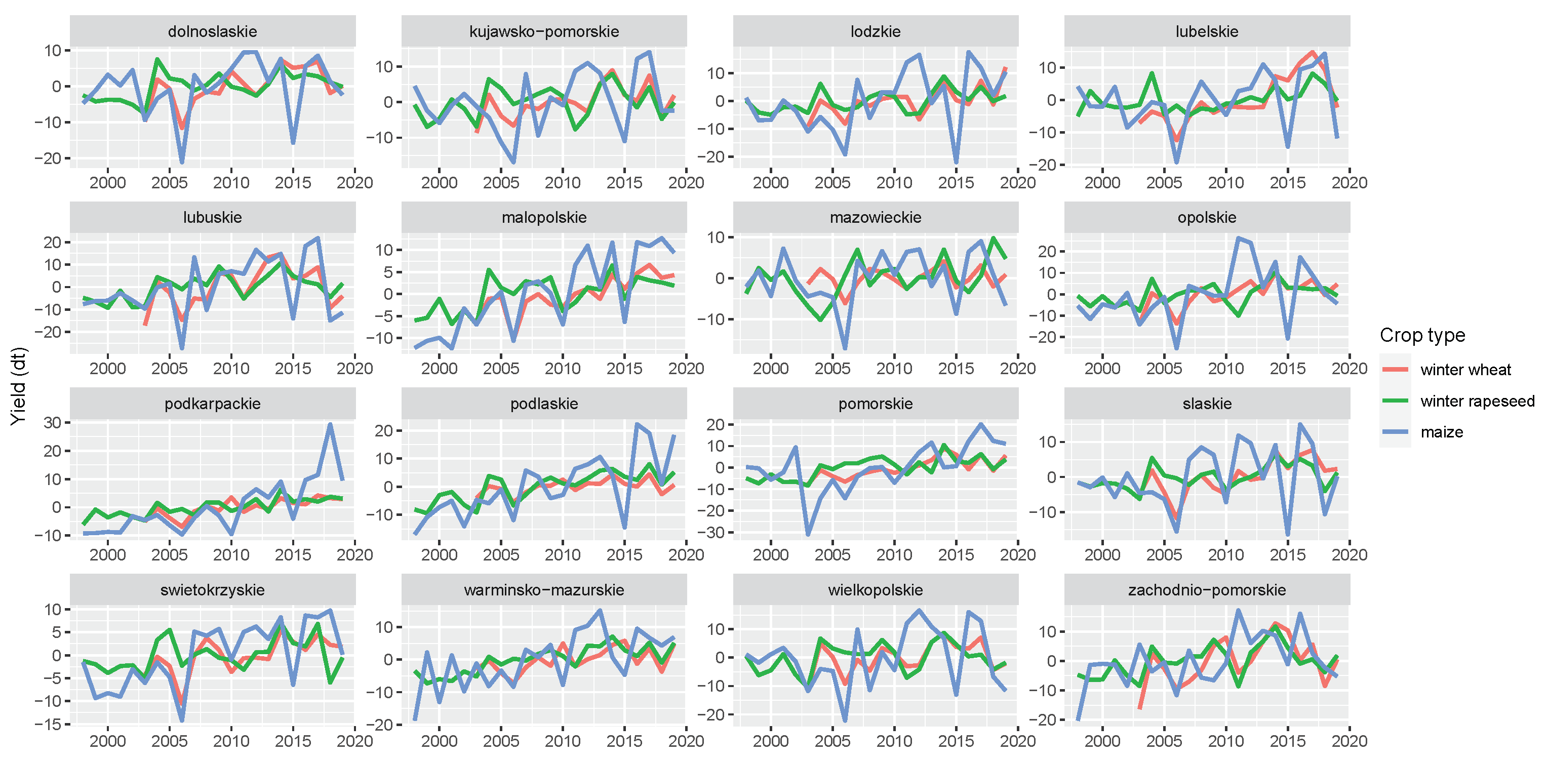
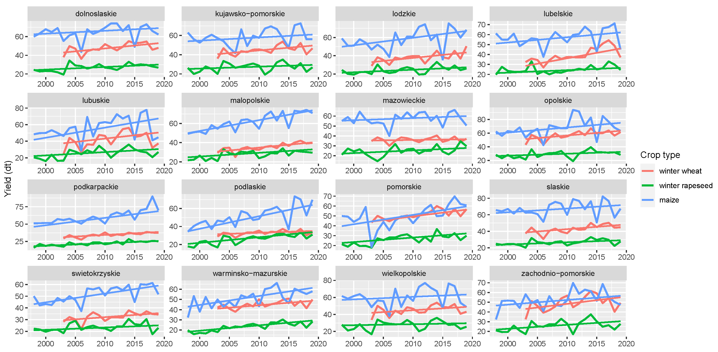
2.4. Crop Yield Statistics
3. Methods
3.1. Spatial Aggregation
3.2. Temporal Smoothing of NDVI Values
3.3. Cross-Calibration of NDVI and LST Products Derived from MODIS and Sentinel-2 Data
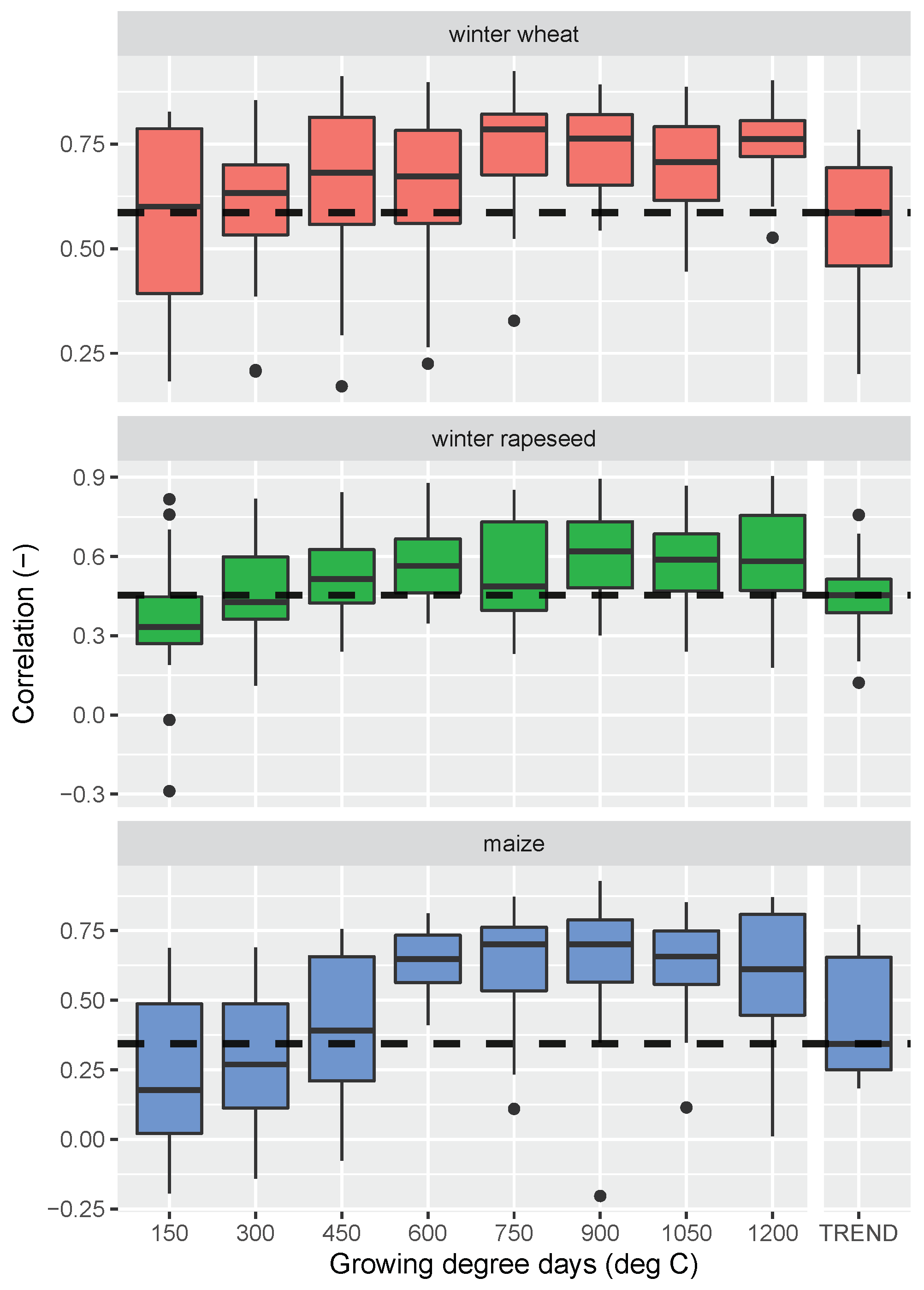
3.4. Resampling of Explanatory Variables from Calendar Time to Thermal Time
3.5. Crop Yield Forecasting
- Minimum, maximum and mean air temperature;
- Surface radiation;
- Accumulated surface radiation since 1 April;
- Soil moisture at 0–7 cm and 7–28 cm levels;
- Precipitation;
- Accumulated precipitation since 1 April;
- ;
- ;
- ;
- ;
- Annual maximum NDVI (which does not correspond to the GDD levels).
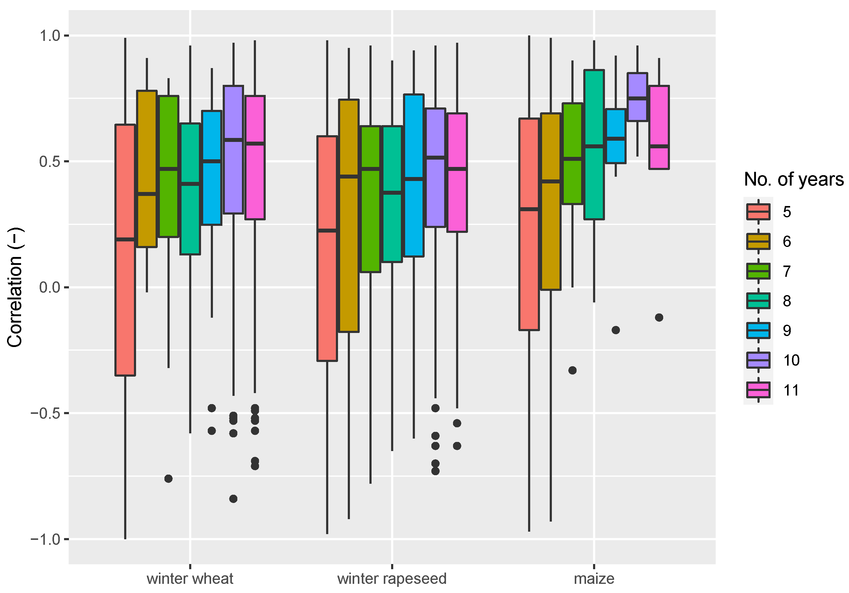
3.6. Validation Approach
4. Results
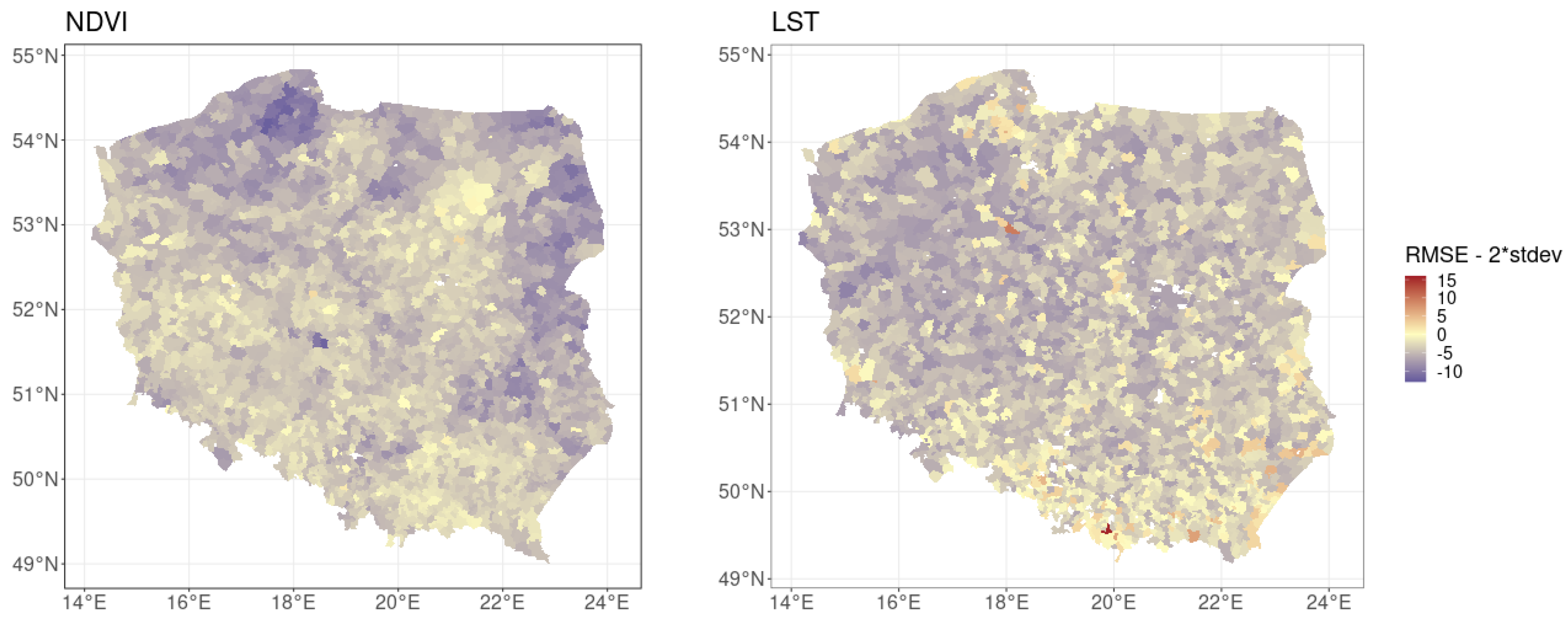
4.1. Accuracy of Cross-Calibration between MODIS and Sentinel-3 Products
4.2. Yield Forecasting Performance
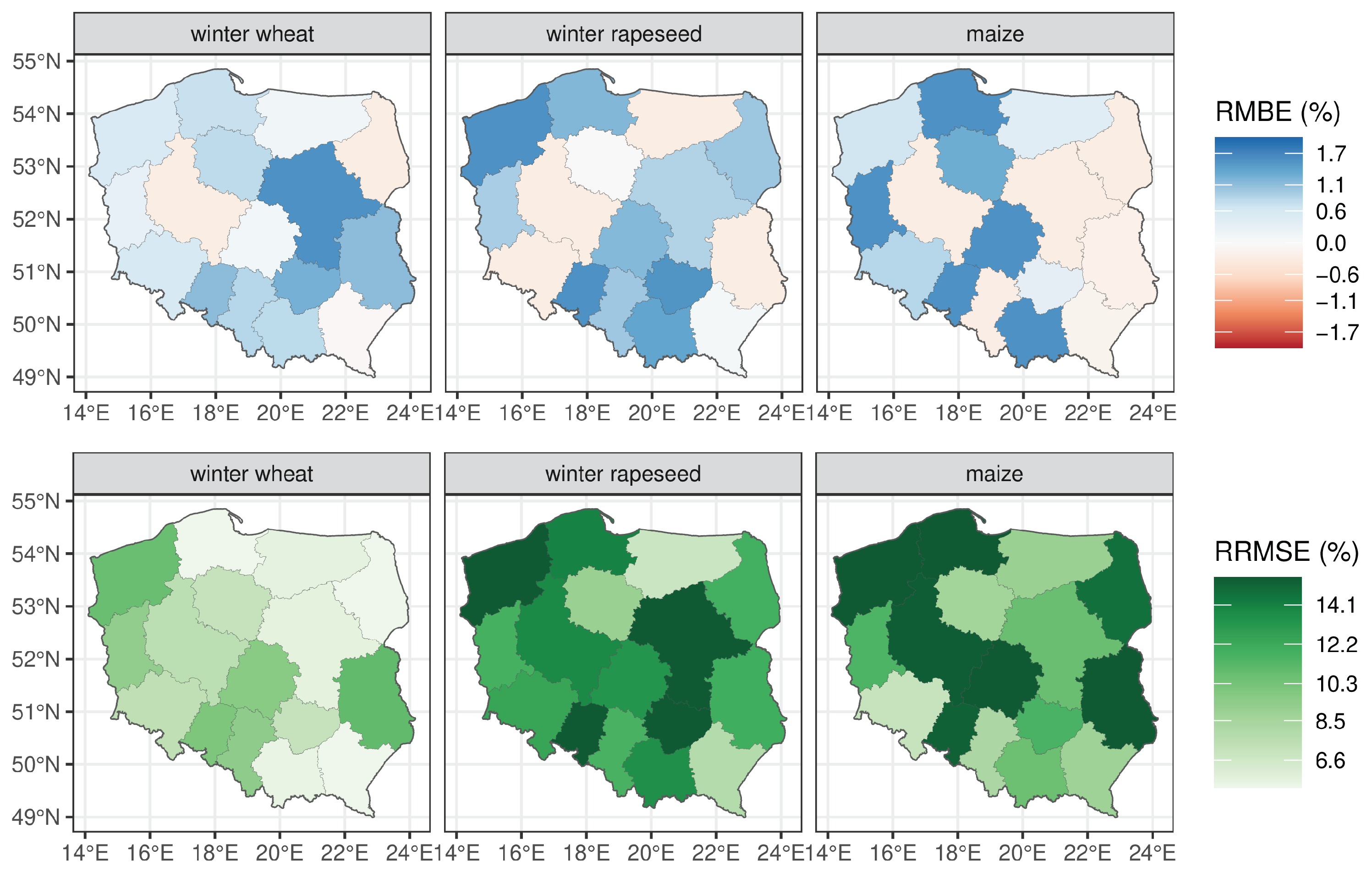
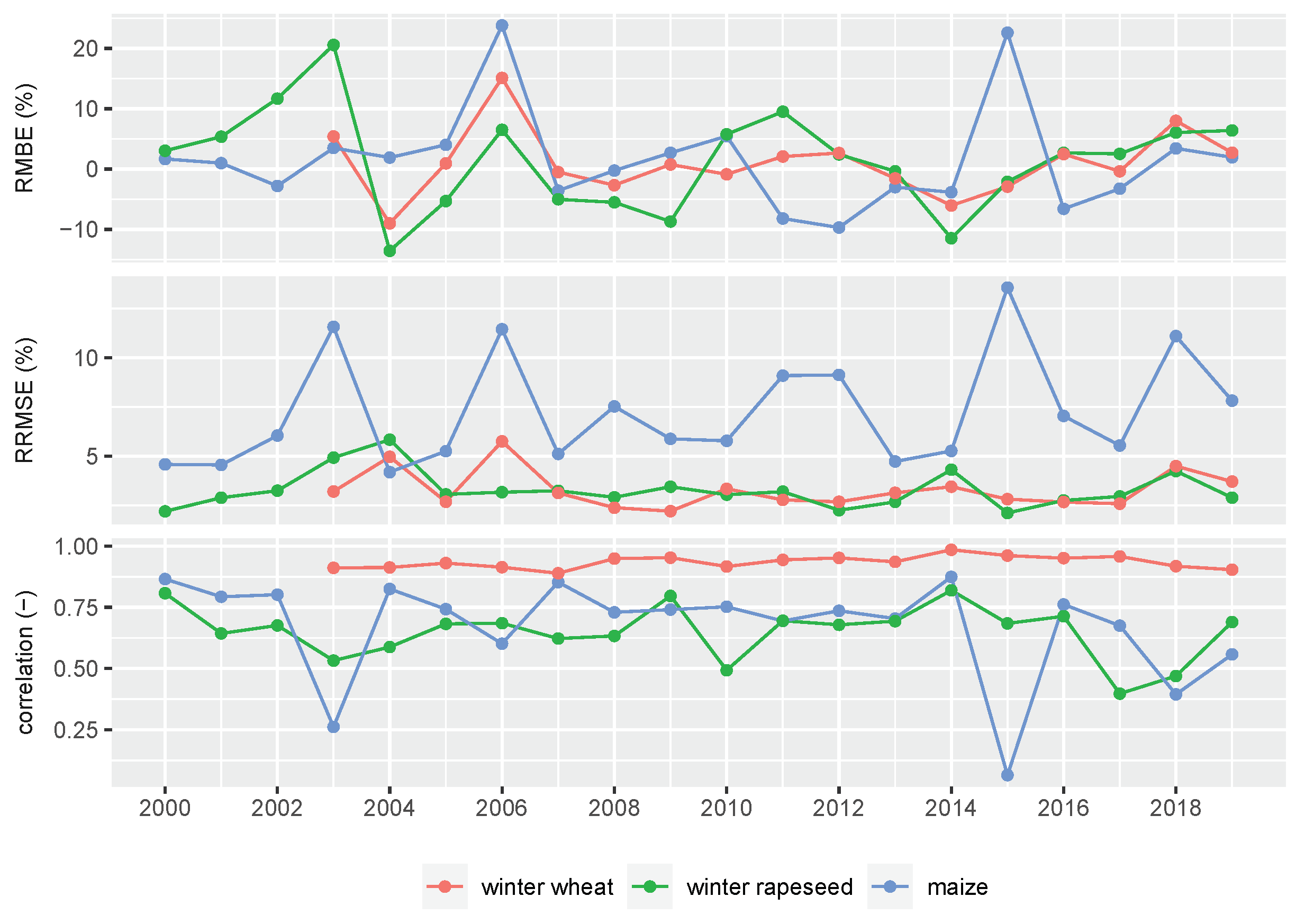
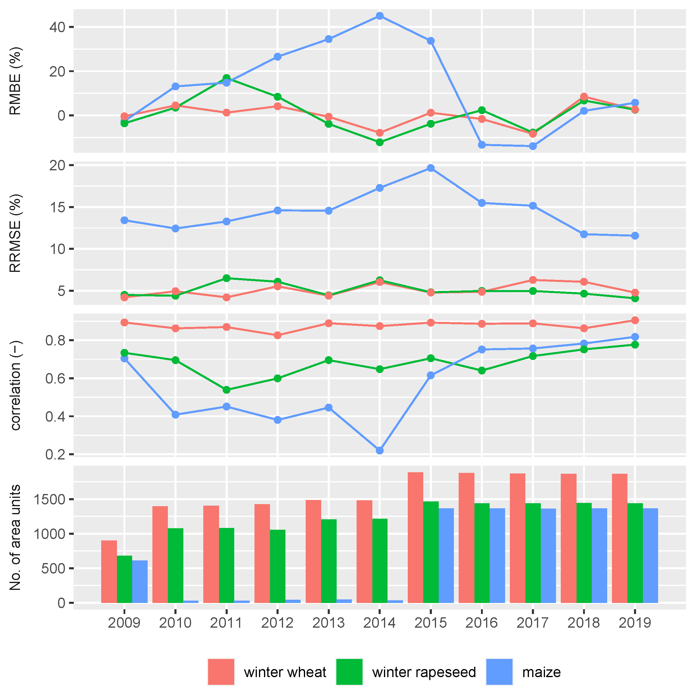
4.2.1. Nuts-2 Level
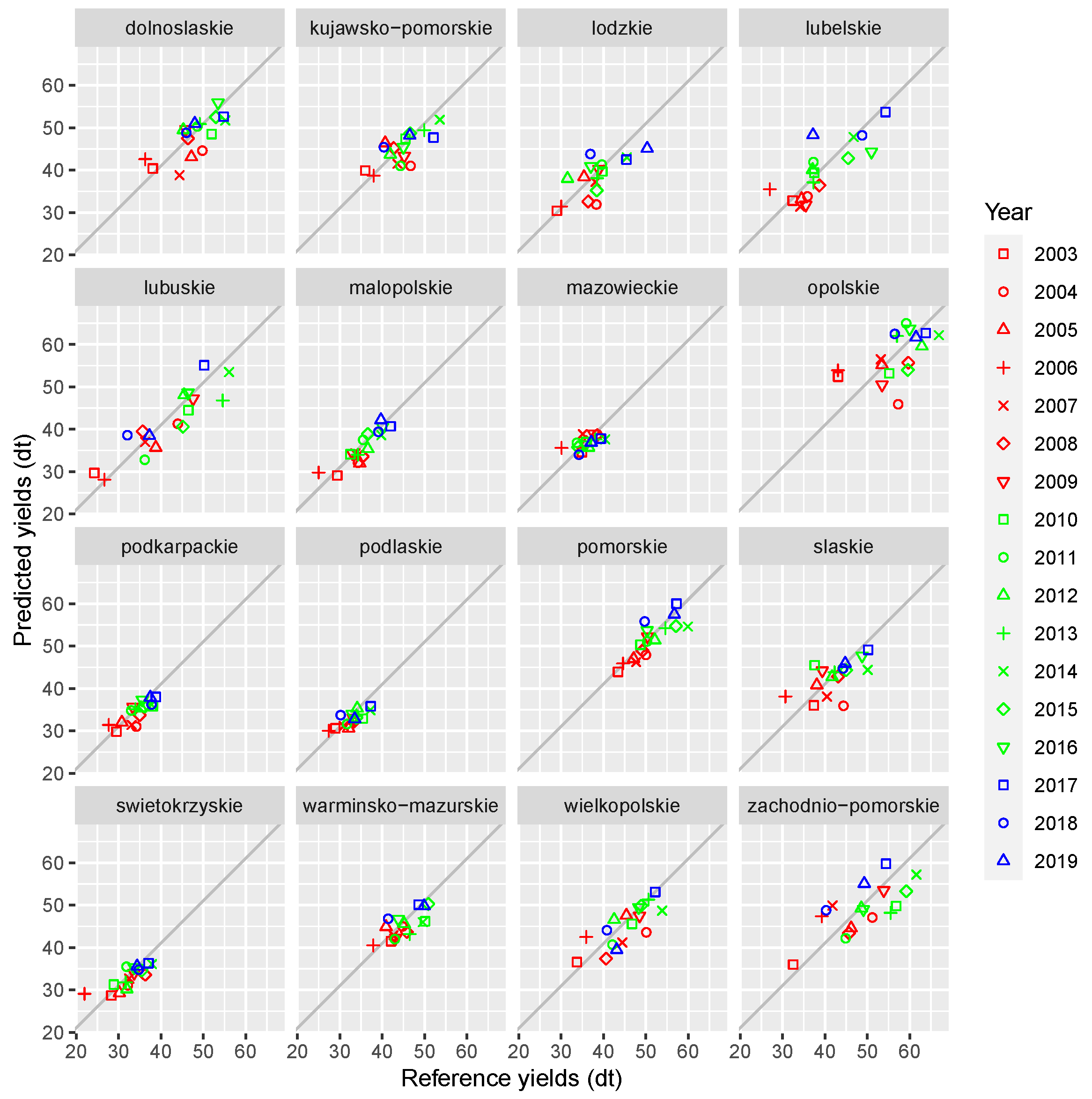
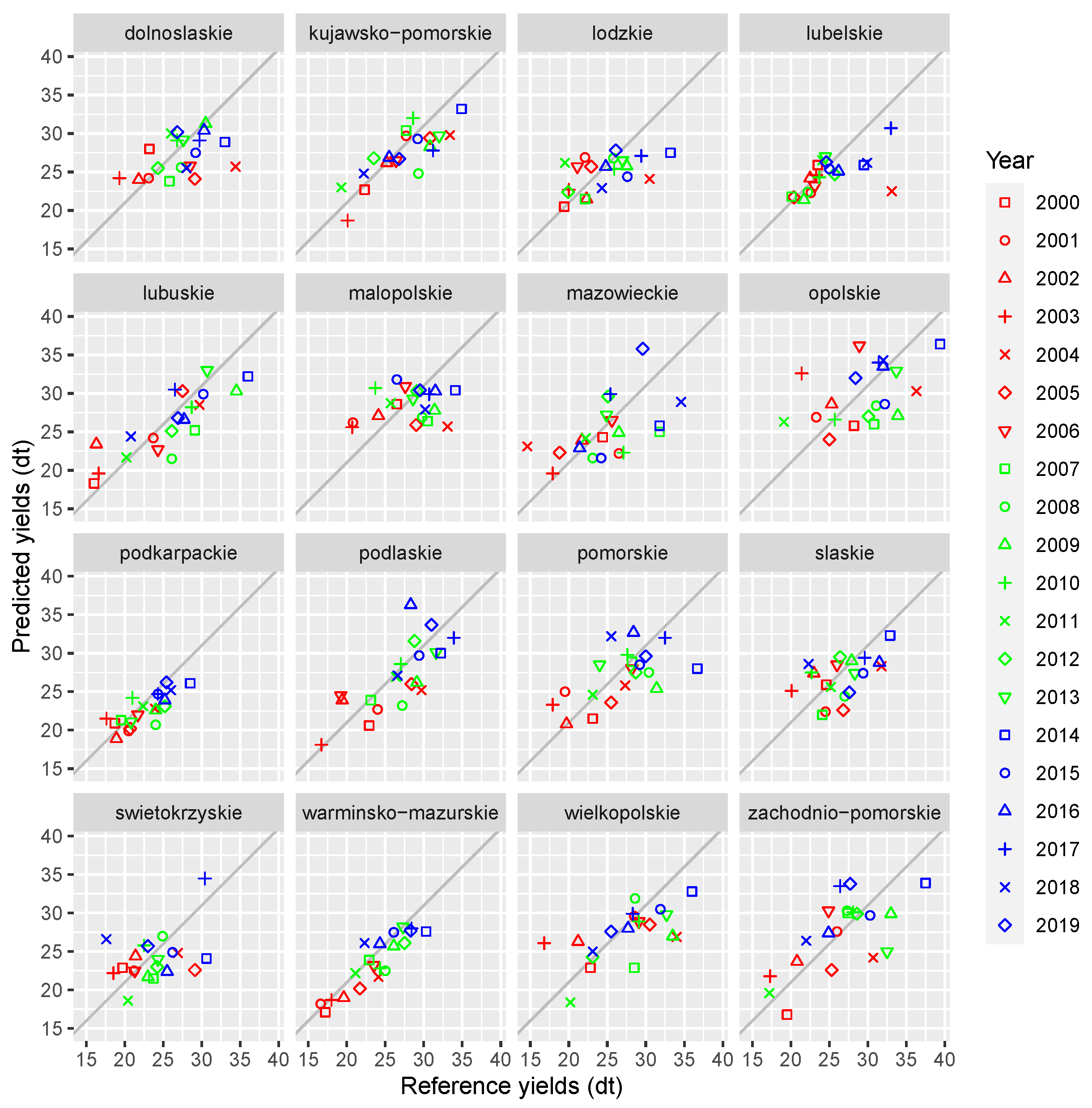
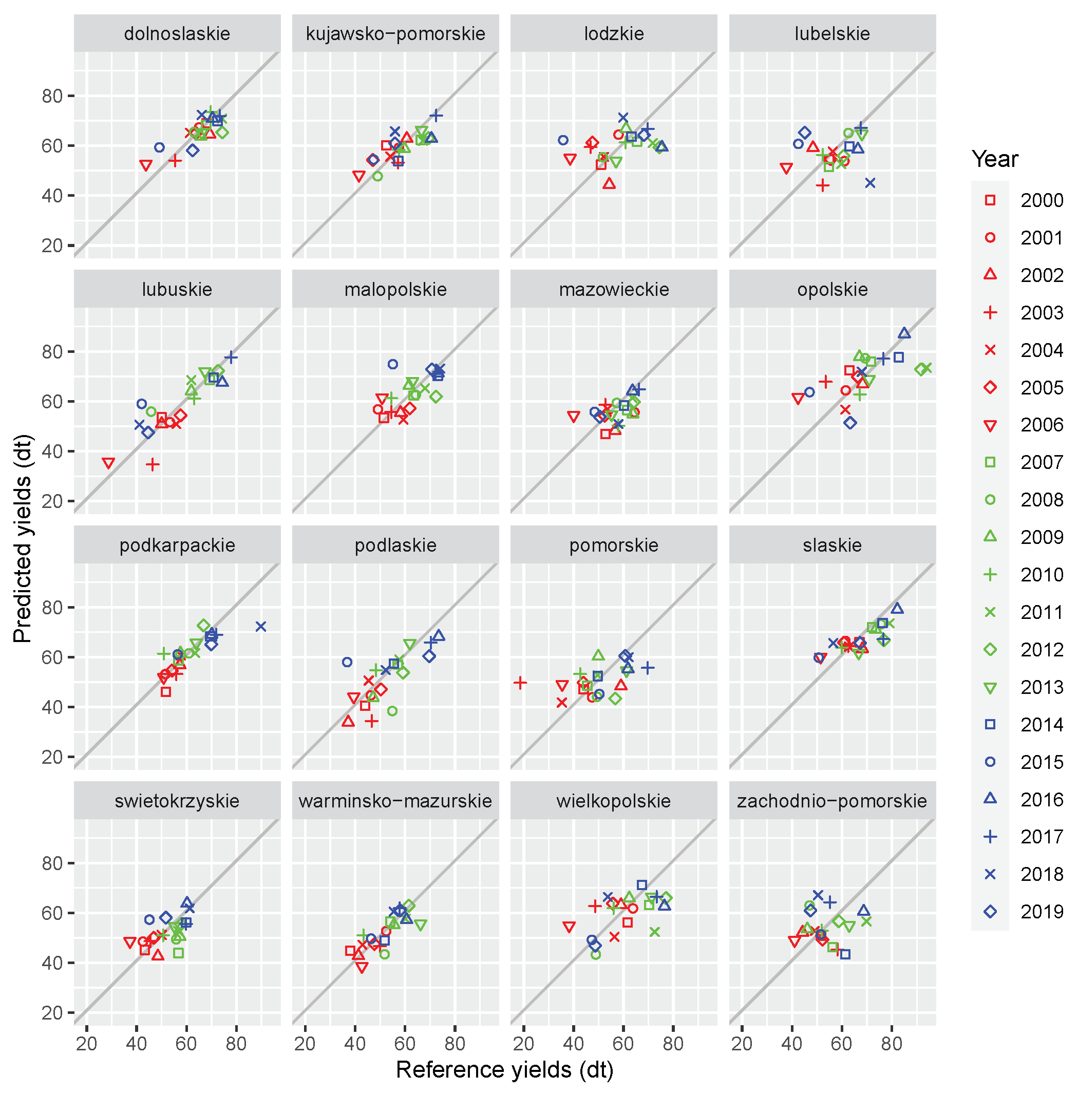
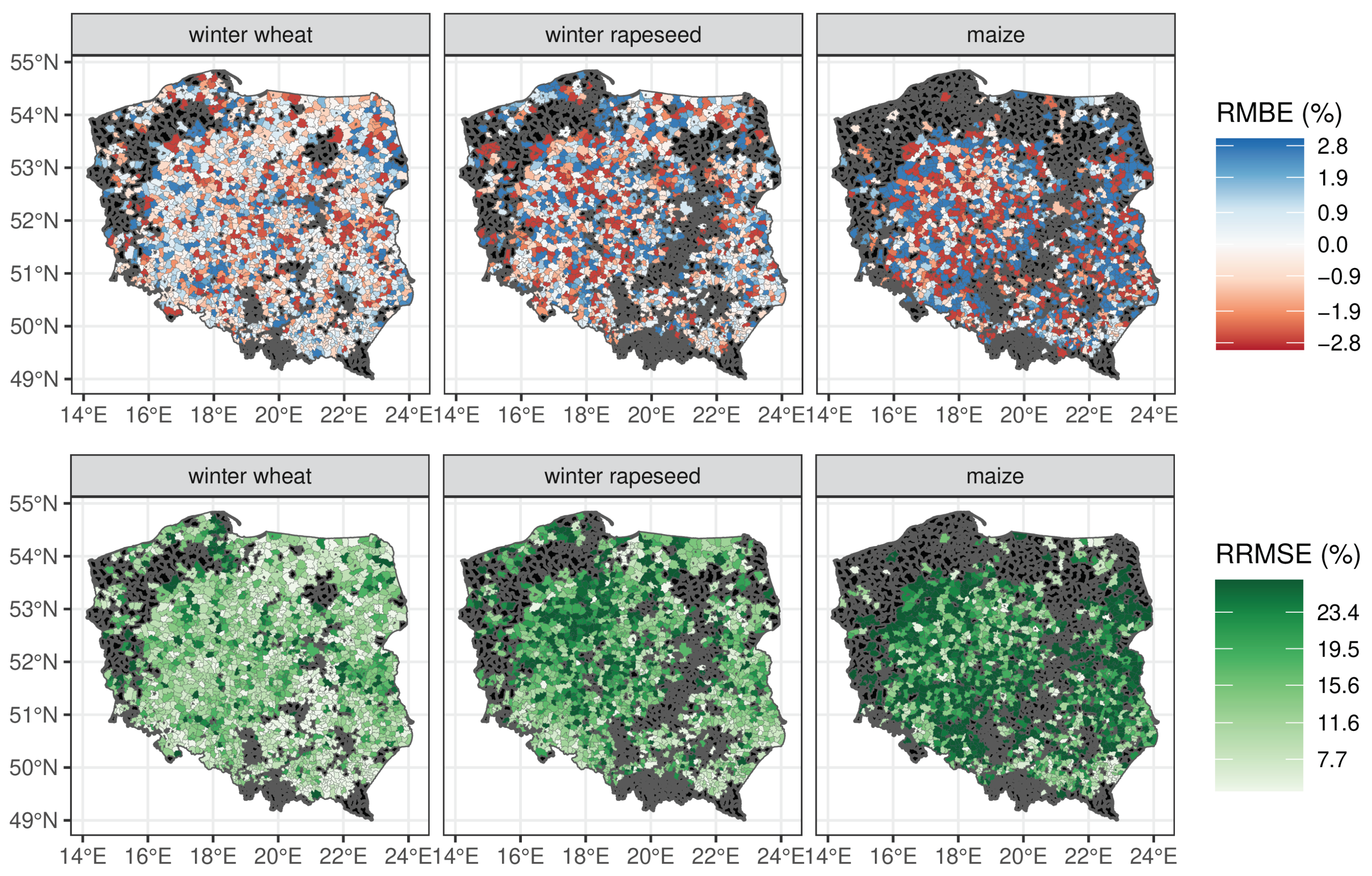
4.2.2. LAU Level
5. Implementation of the Operational System
6. Discussion
6.1. System Performance
6.2. Cross-Calibration of Satellite Indices
6.3. Heterogeneity of Spectral Signatures at the Moderate Spatial Resolution
6.4. Limitation of Agro-Meteorological Indicators
6.5. Applicability of the Crop Yield Forecasting System to Other Areas
6.6. Perspectives
7. Conclusions
Author Contributions
Funding
Institutional Review Board Statement
Data Availability Statement
Conflicts of Interest
References
- Becker-Reshef, I.; Justice, C.; Barker, B.; Humber, M.; Rembold, F.; Bonifacio, R.; Zappacosta, M.; Budde, M.; Magadzire, T.; Shitote, C.; et al. Strengthening agricultural decisions in countries at risk of food insecurity: The GEOGLAM Crop Monitor for Early Warning. Remote Sens. Environ. 2020, 237, 111553. [Google Scholar] [CrossRef]
- Lobell, D.B.; Cassman, K.G.; Field, C.B. Crop yield gaps: Their importance, magnitudes, and causes. Annu. Rev. Environ. Resour. 2009, 34, 179–204. [Google Scholar] [CrossRef] [Green Version]
- Lobell, D.B. The use of satellite data for crop yield gap analysis. Field Crop. Res. 2013, 143, 56–64. [Google Scholar] [CrossRef] [Green Version]
- Mathew, I.; Shimelis, H.; Mutema, M.; Chaplot, V. What crop type for atmospheric carbon sequestration: Results from a global data analysis. Agric. Ecosyst. Environ. 2017, 243, 34–46. [Google Scholar] [CrossRef]
- Turkeltaub, T.; Kurtzman, D.; Russak, E.E.; Dahan, O. Impact of switching crop type on water and solute fluxes in deep vadose zone. Water Resour. Res. 2015, 51, 9828–9842. [Google Scholar] [CrossRef] [Green Version]
- Gilbert, N. One-third of our greenhouse gas emissions come from agriculture. Nature 2012, 31, 10–12. [Google Scholar] [CrossRef]
- Ray, D.K.; Gerber, J.S.; MacDonald, G.K.; West, P.C. Climate variation explains a third of global crop yield variability. Nat. Commun. 2015, 6, 5989. [Google Scholar] [CrossRef] [Green Version]
- Iizumi, T.; Sakai, T. The global dataset of historical yields for major crops 1981–2016. Sci. Data 2020, 7, 97. [Google Scholar] [CrossRef] [Green Version]
- Becker-Reshef, I.; Vermote, E.; Lindeman, M.; Justice, C. A generalized regression-based model for forecasting winter wheat yields in Kansas and Ukraine using MODIS data. Remote Sens. Environ. 2010, 114, 1312–1323. [Google Scholar] [CrossRef]
- Tucker, C.J.; Holben, B.N.; Elgin, J.H.; McMurtrey, J.E. Relationship of spectral data to grain yield variation. Photogramm. Eng. Remote Sens. 1980, 45, 600–608. [Google Scholar]
- Dabrowska-Zielinska, K.; Kogan, F.; Ciolkosz, A.; Gruszczynska, M.; Kowalik, W. Modelling of crop growth conditions and crop yield in Poland using AVHRR-based indices. Int. J. Remote Sens. 2002, 23, 1109–1123. [Google Scholar] [CrossRef]
- Bastiaanssen, W.G.M.; Ali, S. A new crop yield forecasting model based on satellite measurements applied across the Indus Basin, Pakistan. Agric. Ecosyst. Environ. 2003, 94, 321–340. [Google Scholar] [CrossRef]
- Basnyat, P.; McConkey, B.; Lafond, G.P.; Moulin, A.; Pelcat, Y. Optimal time for remote sensing to relate to crop grain yield on the Canadian prairies. Can. J. Plant Sci. 2004, 84, 97–103. [Google Scholar] [CrossRef]
- Kogan, F.; Yang, B.; Wei, G.; Zhiyuan, P.; Xianfeng, J. Modelling corn production in China using AVHRR-based vegetation health indices. Int. J. Remote Sens. 2005, 26, 2325–2336. [Google Scholar] [CrossRef]
- Prasad, A.K.; Chai, L.; Singh, R.P.; Kafatos, M. Crop yield estimation model for Iowa using remote sensing and surface parameters. Int. J. Appl. Earth Obs. Geoinf. 2006, 8, 26–33. [Google Scholar] [CrossRef]
- Moriondo, M.; Maselli, F.; Bindi, M. A simple model of regional wheat yield based on NDVI data. Eur. J. Agron. 2007, 26, 266–274. [Google Scholar] [CrossRef]
- Kowalik, W.; Dabrowska-Zielinska, K.; Meroni, M.; Raczka, T.U.; de Wit, A. Yield estimation using SPOT-VEGETATION products: A case study of wheat in European countries. Int. J. Appl. Earth Obs. Geoinf. 2014, 32, 228–239. [Google Scholar] [CrossRef]
- Johnson, D.M. An assessment of pre- and within-season remotely sensed variables for forecasting corn and soybean yields in the United States. Remote Sens. Environ. 2014, 141, 116–128. [Google Scholar] [CrossRef]
- Shao, Y.; Campbell, J.B.; Taff, G.N.; Zheng, B. An analysis of cropland mask choice and ancillary data for annual corn yield forecasting using MODIS data. Int. J. Appl. Earth Obs. Geoinf. 2015, 38, 78–87. [Google Scholar] [CrossRef]
- Weiss, M.; Jacob, F.; Duveiller, G. Remote sensing for agricultural applications: A meta-review. Remote Sens. Environ. 2020, 236, 111402. [Google Scholar] [CrossRef]
- Kussul, N.; Mykola, L.; Shelestov, A.; Skakun, S. Crop inventory at regional scale in Ukraine: Developing in season and end of season crop maps with multi-temporal optical and SAR satellite imagery. Eur. J. Remote Sens. 2018, 51, 627–636. [Google Scholar] [CrossRef] [Green Version]
- Rao, P.; Zhou, W.; Bhattarai, N.; Srivastava, A.K.; Singh, B.; Poonia, S.; Lobell, D.B.; Jain, M. Using Sentinel-1, Sentinel-2, and Planet Imagery to Map Crop Type of Smallholder Farms. Remote Sens. 2021, 13, 1870. [Google Scholar] [CrossRef]
- Tricht, K.V.; Gobin, A.; Gilliams, S.; Piccard, I. Synergistic Use of Radar Sentinel-1 and Optical Sentinel-2 Imagery for Crop Mapping: A Case Study for Belgium. Remote Sens. 2018, 10, 1642. [Google Scholar] [CrossRef] [Green Version]
- Franch, B.; Vermote, E.; Skakun, S.; Roger, J.; Becker-Reshef, I.; Murphy, E.; Justice, C. Remote sensing based yield monitoring: Application to winter wheat in United States and Ukraine. Int. J. Appl. Earth Obs. Geoinf. 2019, 76, 112–127. [Google Scholar] [CrossRef]
- Lobell, D.B.; Asner, G.P.; Ortiz-Monasterio, J.I.; Benning, T.L. Remote sensing of regional crop production in the Yaqui Valley, Mexico: Estimates and uncertainties. Agric. Ecosyst. Environ. 2003, 94, 205–220. [Google Scholar] [CrossRef] [Green Version]
- Nolasco, M.; Ovando, G.; Sayago, S.; Magario, I.; Bocco, M. Estimating soybean yield using time series of anomalies in vegetation indices from MODIS. Int. J. Remote Sens. 2020, 42, 405–421. [Google Scholar] [CrossRef]
- Doraiswamy, P. Crop condition and yield simulations using Landsat and MODIS. Remote Sens. Environ. 2004, 92, 548–559. [Google Scholar] [CrossRef]
- Vermote, E. MODIS/Terra Surface Reflectance 8-Day L3 Global 250m SIN Grid V061. 2021. Available online: https://lpdaac.usgs.gov/products/mod09q1v061/ (accessed on 20 November 2020).
- Schulzweida, U. CDO User Guide. 2020. Available online: https://code.mpimet.mpg.de/projects/cdo/wiki/Cite (accessed on 20 November 2020).
- Theil, H. A Rank-Invariant Method of Linear and Polynomial Regression Analysis. In Advanced Studies in Theoretical and Applied Econometrics; Springer: Berlin/Heidelberg, Germany, 1992; pp. 345–381. [Google Scholar] [CrossRef]
- Genovese, G.; Vignolles, C.; Nègre, T.; Passera, G. A methodology for a combined use of normalised difference vegetation index and CORINE land cover data for crop yield monitoring and forecasting. A case study on Spain. Agronomie 2001, 21, 91–111. [Google Scholar] [CrossRef] [Green Version]
- R Core Team. R: A Language and Environment for Statistical Computing; R Foundation for Statistical Computing: Vienna, Austria, 2021. [Google Scholar]
- Chen, J.; Jönsson, P.; Tamura, M.; Gu, Z.; Matsushita, B.; Eklundh, L. A simple method for reconstructing a high-quality NDVI time-series data set based on the Savitzky–Golay filter. Remote Sens. Environ. 2004, 91, 332–344. [Google Scholar] [CrossRef]
- Bonhomme, R. Bases and limits to using ‘degree.day’ units. Eur. J. Agron. 2000, 13, 1–10. [Google Scholar] [CrossRef]
- Duveiller, G.; Baret, F.; Defourny, P. Using Thermal Time and Pixel Purity for Enhancing Biophysical Variable Time Series: An Interproduct Comparison. IEEE Trans. Geosci. Remote Sens. 2013, 51, 2119–2127. [Google Scholar] [CrossRef]
- Trudgill, D.L.; Honek, A.; Li, D.; Straalen, N.M. Thermal time—Concepts and utility. Ann. Appl. Biol. 2005, 146, 1–14. [Google Scholar] [CrossRef]
- Kogan, F.N. Global Drought Watch from Space. Bull. Am. Meteorol. Soc. 1997, 78, 621–636. [Google Scholar] [CrossRef]
- Chen, T.; Guestrin, C. XGBoost: A scalable tree boosting system. In Proceedings of the 22nd ACM SIGKDD International Conference on Knowledge Discovery and Data Mining, ACM, San Francisco, CA, USA, 13–17 August 2016. [Google Scholar] [CrossRef] [Green Version]
- Chen, T.; He, T.; Benesty, M.; Khotilovich, V.; Tang, Y.; Cho, H.; Chen, K.; Mitchell, R.; Cano, I.; Zhou, T.; et al. Extreme Gradient Boosting, R Package Version 1.5.0.2. 2021.
- Guyon, I.; Weston, J.; Barnhill, S.; Vapnik, V. Gene Selection for Cancer Classification using Support Vector Machines. Mach. Learn. 2002, 46, 389–422. [Google Scholar] [CrossRef]
- Kuśmierek-Tomaszewska, R.; Żarski, J. Assessment of Meteorological and Agricultural Drought Occurrence in Central Poland in 1961–2020 as an Element of the Climatic Risk to Crop Production. Agriculture 2021, 11, 855. [Google Scholar] [CrossRef]
- Franch, B.; Vermote, E.; Becker-Reshef, I.; Claverie, M.; Huang, J.; Zhang, J.; Justice, C.; Sobrino, J. Improving the timeliness of winter wheat production forecast in the United States of America, Ukraine and China using MODIS data and NCAR Growing Degree Day information. Remote Sens. Environ. 2015, 161, 131–148. [Google Scholar] [CrossRef]
- Paudel, D.; Boogaard, H.; de Wit, A.; van der Velde, M.; Claverie, M.; Nisini, L.; Janssen, S.; Osinga, S.; Athanasiadis, I.N. Machine learning for regional crop yield forecasting in Europe. Field Crop. Res. 2022, 276, 108377. [Google Scholar] [CrossRef]
- Veloso, A.; Mermoz, S.; Bouvet, A.; Toan, T.L.; Planells, M.; Dejoux, J.F.; Ceschia, E. Understanding the temporal behavior of crops using Sentinel-1 and Sentinel-2-like data for agricultural applications. Remote Sens. Environ. 2017, 199, 415–426. [Google Scholar] [CrossRef]
- Skakun, S.; Vermote, E.; Franch, B.; Roger, J.C.; Kussul, N.; Ju, J.; Masek, J. Winter Wheat Yield Assessment from Landsat 8 and Sentinel-2 Data: Incorporating Surface Reflectance, Through Phenological Fitting, into Regression Yield Models. Remote Sens. 2019, 11, 1768. [Google Scholar] [CrossRef] [Green Version]
- Franch, B.; Bautista, A.S.; Fita, D.; Rubio, C.; Tarrazó-Serrano, D.; Sánchez, A.; Skakun, S.; Vermote, E.; Becker-Reshef, I.; Uris, A. Within-Field Rice Yield Estimation Based on Sentinel-2 Satellite Data. Remote Sens. 2021, 13, 4095. [Google Scholar] [CrossRef]
- Tian, F.; Cai, Z.; Jin, H.; Hufkens, K.; Scheifinger, H.; Tagesson, T.; Smets, B.; Hoolst, R.V.; Bonte, K.; Ivits, E.; et al. Calibrating vegetation phenology from Sentinel-2 using eddy covariance, PhenoCam, and PEP725 networks across Europe. Remote Sens. Environ. 2021, 260, 112456. [Google Scholar] [CrossRef]
- Gamon, J.A.; Field, C.B.; Goulden, M.L.; Griffin, K.L.; Hartley, A.E.; Joel, G.; Penuelas, J.; Valentini, R. Relationships Between NDVI, Canopy Structure, and Photosynthesis in Three Californian Vegetation Types. Ecol. Appl. 1995, 5, 28–41. [Google Scholar] [CrossRef] [Green Version]
- d’Andrimont, R.; Verhegghen, A.; Lemoine, G.; Kempeneers, P.; Meroni, M.; van der Velde, M. From parcel to continental scale—A first European crop type map based on Sentinel-1 and LUCAS Copernicus in-situ observations. Remote Sens. Environ. 2021, 266, 112708. [Google Scholar] [CrossRef]
- Woźniak, E.; Rybicki, M.; Kofman, W.; Aleksandrowicz, S.; Wojtkowski, C.; Lewiński, S.; Bojanowski, J.; Musiał, J.; Milewski, T.; Slesiński, P.; et al. Multi-temporal phenological indices derived from time series Sentinel-1 images to country-wide crop classification. Int. J. Appl. Earth Obs. Geoinf. 2022, 107, 102683. [Google Scholar] [CrossRef]
- Song, L.; Guanter, L.; Guan, K.; You, L.; Huete, A.; Ju, W.; Zhang, Y. Satellite sun-induced chlorophyll fluorescence detects early response of winter wheat to heat stress in the Indian Indo-Gangetic Plains. Glob. Chang. Biol. 2018, 24, 4023–4037. [Google Scholar] [CrossRef] [Green Version]


| Name | Source | Temporal Resolution | Spatial Resolution |
|---|---|---|---|
| Satellite indices | |||
| NDVI (-) | MODIS | 8 day | 250 m |
| NDVI (-) | Sentinel-3 | 1 day | 300 m |
| LST (K) | MODIS | 8 day | 1000 m |
| LST (K) | Sentinel-3 | 1 day | 1000 m |
| Agro-meteorological parameters | |||
| Air temperature (K) | ERA-5 | 1 h | 0.25 deg |
| Precipitation (m) | ERA-5 | 1 h | 0.25 deg |
| Surface radiation () | ERA-5 | 1 h | 0.25 deg |
| Soil moisture 0–7 cm () | ERA-5 | 1 h | 0.25 deg |
| Soil moisture 7–28 cm () | ERA-5 | 1 h | 0.25 deg |
| Crop mask | |||
| Fraction of arable land | CLC * 2018 | static | Polygons ** |
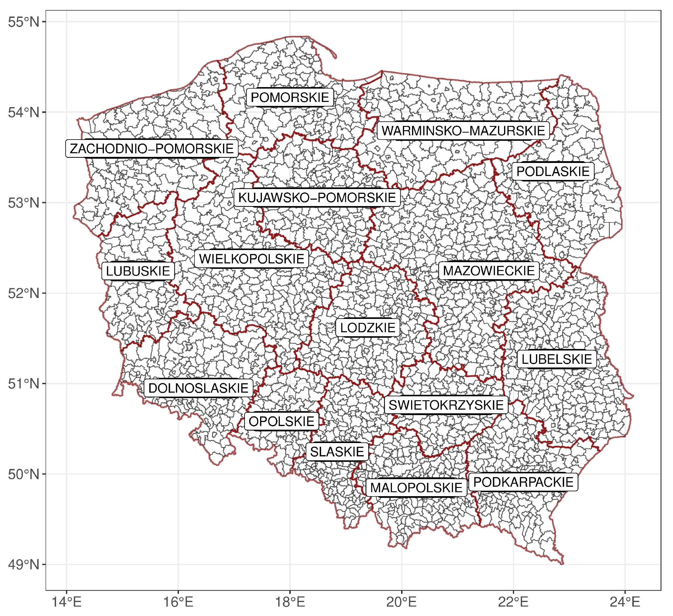
| Administrative units | |||
| NUTS-2/LAU | GUGiK *** | static | Polygons |
| Response Variable | Status | Predictors | MBE | RMSE | EF |
|---|---|---|---|---|---|
| prior to calibration | – | 3.40 | 5.16 | 0.73 | |
| calibrated by RF | , DOY, GDD | 0.07 | 2.95 | 0.91 | |
| prior to calibration | – | −7.16 | 7.83 | −0.65 | |
| calibrated by kNN | , DOY, GDD | 0.00 | 2.51 | 0.84 |
| Crop Type | MBE (dt) | RMBE (%) | RMSE (dt) | RRMSE (%) | (–) | Correlation (r) (–) |
|---|---|---|---|---|---|---|
| Winter wheat | 0.25 | 0.60 | 3.43 | 8.15 | 0.84 | 0.92 |
| Winter rapeseed | 0.19 | 0.71 | 3.39 | 13.03 | 0.47 | 0.69 |
| Maize | 0.37 | 0.63 | 7.76 | 13.32 | 0.51 | 0.71 |
| Crop Type | MBE (dt) | RMBE (%) | RMSE (dt) | RRMSE (%) | (–) | Correlation (r) (–) |
|---|---|---|---|---|---|---|
| Winter wheat | −0.01 | −0.03 | 5.20 | 13.77 | 0.75 | 0.87 |
| Winter rapeseed | −0.02 | −0.07 | 5.09 | 18.80 | 0.45 | 0.67 |
| Maize | 0.07 | 0.12 | 14.89 | 27.36 | 0.48 | 0.69 |
Publisher’s Note: MDPI stays neutral with regard to jurisdictional claims in published maps and institutional affiliations. |
© 2022 by the authors. Licensee MDPI, Basel, Switzerland. This article is an open access article distributed under the terms and conditions of the Creative Commons Attribution (CC BY) license (https://creativecommons.org/licenses/by/4.0/).
Share and Cite
Bojanowski, J.S.; Sikora, S.; Musiał, J.P.; Woźniak, E.; Dąbrowska-Zielińska, K.; Slesiński, P.; Milewski, T.; Łączyński, A. Integration of Sentinel-3 and MODIS Vegetation Indices with ERA-5 Agro-Meteorological Indicators for Operational Crop Yield Forecasting. Remote Sens. 2022, 14, 1238. https://doi.org/10.3390/rs14051238
Bojanowski JS, Sikora S, Musiał JP, Woźniak E, Dąbrowska-Zielińska K, Slesiński P, Milewski T, Łączyński A. Integration of Sentinel-3 and MODIS Vegetation Indices with ERA-5 Agro-Meteorological Indicators for Operational Crop Yield Forecasting. Remote Sensing. 2022; 14(5):1238. https://doi.org/10.3390/rs14051238
Chicago/Turabian StyleBojanowski, Jędrzej S., Sylwia Sikora, Jan P. Musiał, Edyta Woźniak, Katarzyna Dąbrowska-Zielińska, Przemysław Slesiński, Tomasz Milewski, and Artur Łączyński. 2022. "Integration of Sentinel-3 and MODIS Vegetation Indices with ERA-5 Agro-Meteorological Indicators for Operational Crop Yield Forecasting" Remote Sensing 14, no. 5: 1238. https://doi.org/10.3390/rs14051238