Airborne HySpex Hyperspectral Versus Multitemporal Sentinel-2 Images for Mountain Plant Communities Mapping

Abstract

Climate change and anthropopression significantly impact plant communities by leading to the spread of expansive and alien invasive plants, thus reducing their biodiversity. Due to significant elevation gradients, high-mountain plant communities in a small area allow for the monitoring of the most important environmental changes. Additionally, being a tourist attraction, they are exposed to direct human influence (e.g., trampling). Airborne hyperspectral remote sensing is one of the best data sources for vegetation mapping, but flight campaign costs limit the repeatability of surveys. A possible alternative approach is to use satellite data from the Copernicus Earth observation program. In our study, we compared multitemporal Sentinel-2 data with HySpex airborne hyperspectral images to map the plant communities on Tatra Mountains based on open-source R programing implementation of Random Forest and Support Vector Machine classifiers. As high-mountain ecosystems are adapted to topographic conditions, the input of Digital Elevation Model (DEM) derivatives on the classification accuracy was analyzed and the effect of the number of training pixels was tested to procure practical information for field campaign planning. For 13 classes (from rock scree communities and alpine grasslands to montane conifer and deciduous forests), we achieved results in the range of 76–90% F1-score depending on the data set. Topographic features: digital terrain model (DTM), normalized digital surface model (nDSM), and aspect and slope maps improved the accuracy of HySpex spectral images, transforming their minimum noise fraction (MNF) bands and Sentinel-2 data sets by 5–15% of the F1-score. Maps obtained on the basis of HySpex imagery (2 m; 430 bands) had a high similarity to maps obtained on the basis of multitemporal Sentinel-2 data (10 m; 132 bands; 11 acquisition dates), which was less than one percentage point for classifications based on 500–1000 pixels; for sets consisting of 50–100 pixels, Random Forest (RF) offered better accuracy.

1. Introduction

Due to the large variety of environmental conditions in the vertical and horizontal gradients, mountain vegetation has developed specific habitat adaptations. High-mountain plant communities are an important indicator of climate change because they include a wide spectrum of specialized plant species (e.g., endemics) recognized as indicator species [1]. The adaptations are a consequence of highly differentiated vegetation belts, e.g., temperature, sunlight, exposure to high-energy UV radiation, strong, drying winds, water vapor, soil nutrients, and water content. These factors influence the survival strategies of individual species, visible in the plant physiology and morphology [2,3]. When the winters are relatively warm, plants have a chance to survive in harsher conditions, beginning to occupy higher-located habitats, which under normal circumstances would not be available to them, and during colder winters or when the snow cover decreases, plants are exposed to frost, which initiates fungal and insect-related diseases, causing plant dieback [4,5,6]. Such highly adapted habitats should be monitored to understand trends in ecosystem transformations, especially thermal, water, and soil properties [7,8], but it is difficult to monitor mountain areas because of a short growing season, a huge mosaic formed by abiotic and biotic components, and frequent and dense cloud covers hindering the acquisition of good-quality remote sensing images [9,10,11]. Vegetation mapping studies often involve wetlands [12,13], grassland communities [14,15,16], and dune vegetation [17,18] or forests [19,20,21]. Currently, imaging spectroscopy is the most popular remote sensing method for vegetation mapping [22,23]. These data allow the analysis of the physiological state of plants, e.g., the content of photosynthetically active pigments [24,25], water, and cellulose [26], which helps accurately classify plant communities as well as dominant species [27,28]. Often, to improve the classification quality, data obtained from spectral sensors and laser scanning (ALS) need to be fused to analyze the vertical structure of vegetation [29], slope, and aspect, enabling precise identification, e.g., whether the plants are xerothermic or moisture loving [30]. Vegetation indices also help, though they often do not increase accuracy, achieving low scores in variable importance analysis [31,32] because they are based on the same spectral bands [33]. Plant community mapping studies use varying levels of remote sensing, including ground-based data acquired by hyperspectral spectrometers and drones to provide high-resolution imagery, which allows the use of spatial patterns and classification by deep learning methods [34]. These are mostly local case studies, which narrow down the study area significantly [35,36]. Alternatively, data acquired from the airborne level through hyperspectral imaging can be used. This is an effective method, but cost and aircraft availability prevent continuous and repeatable monitoring. In addition, hyperspectral sensors made by various manufacturers have different technical parameters, characteristics, and construction, making them different, and thus their results are not fully repeatable. One of the solutions may be satellite long-term remote sensing missions [37], e.g., Landsat, but the revisit time, cloud covers, and lower resolution hinder the identification and detailed examination of plant communities [38]. A solution may be images acquired by Sentinel-2 satellites, which thanks to frequent revisits, good spatial resolution, and channels designed for vegetation studies (e.g., red edge) provide a high potential for monitoring mountain vegetation. The mission is becoming increasingly important for vegetation studies. Further 2C and 2D satellites are being designed with the same Multispectral Instrument (MSI), enabling multitemporal analyses and repeatable monitoring [39,40]. Sentinel-2 is being increasingly used in vegetation studies, for example, in biodiversity research [41], to identify community health [42], and for identification [43]. Freely available data, support from ESA, and continuous development and improvement make it one of the best satellites for environmental research today.

Various libraries in open programing languages provide relatively common access to leading algorithms for the classification of hyperspectral and satellite images. Kwan et al. [44] proposed an interesting comparison of vegetation and non-vegetation mapping (15 classes of land cover) based on advanced classifiers [45]. For this purpose, reference data [46] and hyperspectral images (144 bands) were used. For vegetation classes, the authors used 190-pixel-based training sets and reference patches oscillated between 505 and 1056 pixels. The best algorithms identified were Joint Sparse Representation (JSR; overall accuracy 87%), Convolutional Neural Network (CNN; overall accuracy 86%), and Support Vector Machine (SVM; overall accuracy 86%) [44]. Adaptive Subspace Detection (ASD), Matched Subspace Detection (MSD), Reed-Xiaoli Detection (RXD), Kernel MSD (KMSD), Kernel ASD (KASD), Kernel RXD (KRXD), and Sparse Representation (SR) offered comparatively inferior results [44]. Similar observations were noted by Li and Stein [47], who achieved the best results for the Bayesian classifier via Graph Convolutional Networks (GCNs), with an overall accuracy of 85–87%, followed by SVM, with an accuracy of 76–80%, and RF, with an accuracy of 67–68%; RF offered 93% accuracy for green areas and GF2 satellite images [47]. Zagajewski [48] used DAIS 7915 airborne hyperspectral images (79 spectral bands), classified by fuzzy ARTMAP, allowing the identification of 41 plant communities of the Tatra National Park, depending on the data set (40 of the most informative or 20 MNF bands); the overall accuracy oscillated between 84% and 89%. For plant communities, the highest producer accuracy achieved was 93% and user accuracy was 84%, while the average accuracy of all classifications was 86% and 75%, respectively. Moreover, the tests confirmed that the optimal pattern for the neural network training would involve at least 400 pixels of each class and 40 spectral bands. The classifications carried out on the MNF data offered accuracies lower by several percentage points, but the data processing time was shorter by 2–3 times. Importantly, the analysis carried out using DTM derivatives helped achieve results that were enhanced by about 10 percentage points, but for xerothermic communities or areas with long snow deposition, the obtained accuracy improved by up to 30 percentage points [48]. Adding the DEM layer to the Sentinel-2 data set improved the classification accuracy of forest species by 2–3% [49]. Studies based on feed-forward multilayer perceptron (MLP) and airborne APEX hyperspectral images (288 spectral bands with a 3 m spatial resolution) helped identify woody species with a median overall accuracy (OA) of 87%, with spruce identified with 93% accuracy (producer accuracy (PA)), beech with 88% accuracy, birch with 83% accuracy, and pine (which is an introduced species and creates heterogeneous patterns with different species) with 75% accuracy [10]. Bigger reference polygons were used for the classification of Sentinel-2 and Landsat 8 images. The best results were achieved for the SVM RBF classifier (86.5% OA; the analyzed species had results lower by a few percentage points) [11]. In subalpine and alpine zones, 22 vegetation communities were identified based on the SVM and the same APEX data with an OA of 84% [27], and based on the Sentinel-2 images, only eight types of plants could be mapped (larger and homogenous patches), scoring 80% median overall accuracy (OA) for multitemporal images and 70–72% OA for a single-date scene [50]. However, when multitemporal Sentinel-2 data were used to map tree species classification (RF classifier) for a single image depending on the period, 87% OA was achieved for April and October. The combination of two images (spring and autumn) improved the OA to 90%. Adding three images (one spring and two autumn images) resulted in a slight increase in the OA values to 92%; for four images (two spring and two autumn images), the OA was 92%; the highest values were achieved for five images: 92% OA. Using all images did not improve the accuracy of classification of forest species (92% OA) [49]. Therefore, in multitemporal analyses, it is important to correctly select images that differentiate the phases of the vegetation period and thus the spectral features that differentiate the studied communities or species.

The above literature review has confirmed the importance of monitoring the boundaries and condition of plant communities and that occurrence is determined by thermal, water, and trophic properties (in the first step, changes lead to disturbances in thin soil layers [51], which have limited possibilities to neutralize changes). Understanding and monitoring processes taking place in mountain areas is also regulated by law. For example, the European Union undertook habitat monitoring initiatives through Habitats Directive in programs such as the European Union Nature Information System (EUNIS) and habitat classification (or Natura 2000) [52]. A solution presents methods based on satellite images. Despite the images having lower spectral, radiometric, and spatial resolution, satellites often provide freely available data and allow the multitemporal acquisition of images, enabling the monitoring of vegetation changes, which depend on their unique species traits. Sentinel-2 images, whose pixel size is comparable with tree crown sizes, allow for classification results comparable with airborne data [49]. Small, often endemic species remain a problem. Some of them, together with other objects, form heterogeneous patches, making their identification difficult. However, the dynamics of changes in dominant communities help assess the degree of changes, but satellite images are a data source that is objective and repeatable over time and allows for a retrospective assessment of large areas or areas located in different parts of continents. Our previous land cover analyses indicate a greater potential of Sentinel-2 images over Landsat 8 images [11,53]. Following this idea, in this article, we wanted to compare airborne HySpex hyperspectral and Sentinel-2 satellite images to classify the dominant mountain vegetation communities of the Western Tatra Mountains. Though HySpex images should have a much better information content, we used multitemporal Sentinel-2 data, which present different stages of vegetation, allowing the differentiation of unique spectral characteristics of species constituting the communities. Moreover, it should be possible to analyze the species diversity of subalpine and alpine ecosystems, which should complete the whole process of growth, reproduction, and seeding within 2–3 months of the growing season, because at the end of August or the beginning of September, local frosts in the highest parts of mountains stop vegetation. From a practical point of view, a key element is comparing the impact of training and verification set sizes on obtained accuracies. Estimating the size of reference-verified patterns for reliable results is an important task. This task is difficult due to terrain denivelations, difficult access to many parts of protected areas, high variability of weather conditions, as well as limited access to Global Navigation Satellite Systems (GNSS) or mobile telephony signals, making it difficult to correctly locate selected polygons due to high rock walls or dense forests in valleys.

To sum up, the innovative element of the study is assessing the usefulness of multitemporal Sentinel-2 data compared to that of mono-temporal airborne HySpex images for monitoring dominant communities, including initial phases of cryptogamic plant communities through scree communities and shrubs and ending with deciduous and coniferous forests, which are partly attacked by bark beetles. An important issue is assessing hyperspectral data compression algorithms, because 16-bit HySpex images with a spatial resolution of 2 m recorded in 430 spectral bands significantly burden classification processes; a similar problem appears using multitemporal Sentinel-2 images. This is why it is so important to choose the right data set and methods that will enable highly accurate plant community classification and ensure continuous monitoring of these areas, especially when these are protected areas and difficult to access for field research.

2. Materials and Methods

2.1. Study Area

The Tatra Transboundary Biosphere Reserve, one of the most floristically valuable alpine areas, covers areas of the Polish Tatrzański Park Narodowy (TPN) and the Slovak Tatranský Národný Park (TANAP). The area is a subject of numerous vegetation studies [54], based on a fixed network of surveying polygons [55] on which phytosociological mapping is undertaken using the Braun–Blanquet method [56]. The study area was the western part of Tatra Mountains (Western Tatras) located in the Polish Tatra National Park, extending over an area approximately 17 km in length and 7–10 km in width, covering approximately 115 km² (Figure 1). Tatra Mountains are one of the most valuable areas in Europe, listed in the UNESCO Man and Biosphere Reserve (1992) and Natura 2000, characterized by alpine conditions, high biodiversity, and endemic species. Climate conditions are characterized by mean yearly temperature variations from +6 °C in the lowest parts to 0 °C in the highest parts [57]. The long duration of snow cover shortens the vegetation period (from 90 days on the highest part to 180 days on the lowest part), and strong foehn winds (speed 60–80 m/s) often damage forest stands and windfalls. Mean annual precipitation varies from 1140 mm in the lowest part to 1809 mm in the highest part [58]. The main ridge is the boundary of the European watershed (Baltic and Black Sea), and hydrography is characterized by a dense river network. The soil is mainly composed of lithosols on a limestone or granite base, which determines the plant communities. High altitudes (from 770 to 2499 m a.s.l.) and steep slopes make access difficult.

The flora of the park is rich, representing many rare and endemic species. The vegetation of Tatra Mountains is characterized by altitudinal zonation (Figure 2). In the case of forests, the trees were mass harvested for metallurgy needs even in the 19th century. Over time, spruce trees have been manually planted, often inconsistent with the habitat, focusing on the wood growth rate. As a result, now, some large patches of trees are dying due to bark beetle gradation [59,60]. However, intense natural succession is also in process, where deciduous species (beech, maple, mountain ash, etc.) grow under the spruce canopy. The alpine meadows are also subject to numerous transformations, e.g., due to pasture increasing nitrogen compounds in the soil, and intense tourist traffic in summer causes turf damages, leading to soil and trail erosion by trampling. This has opened up space for expansive and invasive species [4,61,62]. The dwarf pine, which grows intensively, is a danger for alpine grasslands. In recent years, park employees have observed reduced snow covers, resulting in frosting of the mountain pine tops and causing diseases in selected clumps.

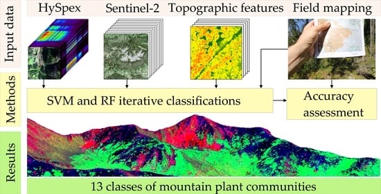
2.2. Research Schema

Multitemporal satellite images, hyperspectral airborne data, as well as LIDAR data derivatives (digital terrain model, normalized digital surface model, and slope and aspect maps) were used to make the model more informative and support the process of identifying communities growing in different belts. The R language Random Forest and Support Vector Machines with radial kernel (RBF) were implemented as machine learning algorithms due to the high-quality results achieved [11,53]. The basis for the selection of training and verification polygons was the official vegetation map of the Polish Tatra National Park, based on which a field campaign was conducted by the authors to identify large and homogenous polygons. The patterns are located in all belts in the whole Polish research area. An iterative classification method was used to limit the randomness of choosing training and verification patterns. All classifications were carried out 100 times, selecting the randomized patterns each time. The final stage was the selection of the set offering the highest accuracy (Figure 3).

2.3. Airborne and Satellite Input Data

Hyperspectral imagery for the Tatra National Park was acquired by HySpex airborne imaging spectrometers (HySpex, Norsk Elektro Optikk AS, Oslo, Norway) located on a Cessna 402B aircraft owned and operated by the MGGP Aero company. Data were acquired in September 2019 and processed atmospherically and geometrically by MGGP Aero (

Table 1. Hyperspectral sensor specification. The average sensor overflight was 2700 m a.s.l. and the final spectral resolution was 2.0 m [28]. Explanations: HySpex VNIR 1800: visible and near-infrared in the range of 400–1000 nm (VNIR); HySpex SWIR-384: short-wave infrared–930–2500 nm (SWIR).

Sensor	HySpex VNIR-1800	HySpex SWIR-384
Spectral range	416–995 nm	954–2510 nm
Spatial pixels	1800	384
Number of spectral bands	163	288
Spatial resolution	1.0 m	2.0 m
Field of view (FOV) across the track	17–34°	16–32°
Instantaneous field of view (IFOV)	0.01–0.04°	0.04–0.08°
Full width at half maximum (FWHM)	3.26 nm	5.45 nm

) based on the ATCOR and the PARGE software [63]. The authors acquired the field reference spectra for atmospheric corrections based on the ASD FieldSpec 4 measurements of homogenous large patterns, e.g., parking places, water bodies, and open ground on cross trails. The field-acquired data were resampled to the HySpex spectral resolution and then compared with responsible pixels after atmospheric correction. The calculated differences oscillated around a root-mean-square error (RMSE) of 0.08.

Based on HySpex 430 hyperspectral bands, minimum noise fraction transformation was performed in ENVI 5.1 software. Then, based on the analysis of eigenvalues, the 30 most informative channels from the MNF data set were selected for further investigation.

Laser scanning data with a density of 8 points/m² were acquired in September 2019 with the Riegl VQ780i sensor with a 50° field of view (FOV) and a spectral range of 1064 nm. Light detection and ranging (LIDAR) data were processed in LAStools software to generate a digital terrain model (DTM) and a digital surface model (DSM) with a 0.5 m resolution. On the basis of the DTM and the DSM, topographic-derived products, such as nDSM, slope, and aspect products, were developed in the raster package [64]. Topographic features (TFs) such as DTM, nDSM, and slope and aspect maps were resampled by the nearest neighbor method to a 2 m pixel size (hyperspectral data) and 10 m (satellite data) to match the image grid of the respective data sets.

The study area covers one granule of Sentinel-2 (34 UDV) available from two orbits (36, 79), allowing image acquisition every 2–3 days. Sentinel-2 images (projection: UTM 34N; EPSG: 32634; processing level-2A) were retrieved automatically using the sen2r package [65] via the Copernicus Open Access Hub. The average cloud cover for the 34 UDV granules from 2015 to 2020 was 59.4%. Due to the short growing season, the long-lasting snow cover, and the significant cloud cover associated with mountainous areas, the available cloud-free period for 2019–2021 was between August and October, when imagery was acquired. The selected scenes have a low cloud cover (less than 1.1%) and are without cloud shadows (

Table 2. Used Sentinel-2 satellite images (granule: 34 UDV). Explanations: 34 UDV–granule identifier; 2A, 2B–series of the Sentinel-2 satellites.

Date	Sentinel-2 Satellite	Track	Cloud Coverage (%)
15 September 2019	2A	79	0.33%
22 September 2019	2A	36	0.06%
17 October 2019	2B	36	0.27%
25 October 2019	2A	79	0.01%
22 August 2020	2B	36	0.24%
4 September 2020	2B	79	1.10%
9 September 2020	2A	79	0.03%
14 September 2020	2B	79	0.72%
21 September 2020	2B	36	1.11%
9 September 2021	2B	79	0.05%
9 October 2021	2B	79	0.04%

). Images were verified for possible distortion. ESA SNAP 7.0.4 and Sentinel-2 Toolbox (S2TBX) software were used to process the images; pixels of 20 and 60 m bands were resampled to the pixel size of 10 m using the nearest neighbor method. Then, the multitemporal scenes were stacked into a single file. Atmospheric corrections are of high quality for mountainous areas in a level-2A product and do not exceed a root-mean-square error (RMSE) of 4–7% [53].

2.4. Reference Data, Classification, and Accuracy Assessment

Reference data were collected during the September 2021 field campaign, during which, based on the official map of the park’s vegetation, the authors identified homogeneous polygons of the studied plant communities with a size 2–3 times larger than the 20 m pixel of the Sentinel-2 image. Then, 13 classes representing dominant plant communities as well as the surface water were field verified. The data were drawn on a high-resolution (0.12 m) CIR orthophoto map draped on the normalized digital surface model (0.5 m), helping identify the most accurate polygons for classification (

Table 3. Classes selected for mountain vegetation mapping and their general characteristics.

Acronym	Class	Description
RS	Rocks and scree communities	Vegetation growing on a loose bedrock or bare rock (initial phases of cryptogamic plant communities, epilithic lichens, and scree communities)
LA	Luzuletum alpino-pilosae	Alpine grasslands
OD	Oreochloo distichae-Juncetum trifidi	Alpine grasslands
FV	Festuco versicoloris Agrostietum	Alpine grasslands
CA	Calamagrostietum	Alpine grasslands
DF	Deschampsia flexuosa community	Alpine grasslands
ON	Other non-forest vegetation	Vegetation of mountain pastures and communities in transition
LO	Low shrubs	Vaccinium myrtillus, Empetrum nigrum and Calluna vulgaris
PM	Pinetum mugo carpaticum	Subalpine dwarf pine shrubs
MS	Montane spruce forests	Coniferous forests composed of Picea abies and an admixture of Abies alba
SN	Snags	Damaged Norway spruce (Picea abies)
DE	Deciduous forest	Fagus sylvatica, Acer pseudoplatanus
WA	Water	Stream and mountain lake waters

and

Table 4. Size of the set used for classification.

Class	Total Polygons	Total Pixels
		HySpex/MNF	Sentinel-2
Rocks and scree communities	18	579	36
Luzuletum alpino-pilosae	19	844	44
Oreochloo distichae-Juncetum trifidi	59	4465	161
Festuco versicoloris-Agrostietum	4	235	11
Calamagrostietum	13	1004	34
Deschampsia flexuosa community	15	233	37
Other non-forest vegetation	16	10,285	373
Low shrubs	58	4529	192
Pinetum mugo carpaticum	52	15,627	561
Montane spruce forests	66	33,005	1200
Snags	38	7750	263
Deciduous forest	25	9757	339
Water	6	5587	206
Total	389	93,900	3457

). As reference polygons, compact and homogeneous surfaces were selected (Figure 4). Almost 400 field polygons were prepared (Table 4).

Then, using the R language 4.0.3 [66], pixel values were extracted from the data using the raster and rgdal [67] packages. Hyperparameter tuning by the grid search 10-fold cross-validation method was performed on the individual data sets (HySpex, MNF, Sentinel-2) to find the optimal values of Random Forest [68] and SVM radial kernel classifiers [69,70]. Reference data were split by stratified random sampling in a 50:50 ratio into a test set and a training set (Table 4). During splitting, it was ensured that pixels from a single polygon were included in the training or test set to ensure their independence and non-spatial correlation [71]. An iterative accuracy assessment [72] procedure was applied, during which the classification procedure was repeated 100 times, assessing the overall accuracy (OA), the kappa coefficient [73], producer and user accuracy (PA and UA) [74], and the F1-score (F1) for all classes each time based on randomized selected verification pixels from the validation set [75,76]. It helped visualize all results using box graphs presenting the median with a 95% confidence interval and first and third quartiles (Q1, Q3), between which is the interquartile range (IQR). The minimum and maximum values represent, respectively, Q1 − 1.5 × IQR and Q3 + 1.5 × IQR. The trained classifier from the iteration that achieved the highest mean F1-score accuracy for all classes was used to prepare vegetation distribution maps and error matrices.

For the final analysis, accuracy comparisons were mainly made based on the F1-score, which is a combination of producer and user accuracy. The F1-score provides higher objectivity than the overall accuracy, which can hide the performance of individual classes by under- or overestimating the results, especially when the validation data set is unbalanced [77,78]. To assess the accuracy, the kappa measure was dropped because this coefficient has a high correlation with the overall accuracy and thus the redundancy of information is doubled [79].

3. Results

Reviewing the results achieved from all classification scenarios, (a) RF and SVM classifiers, (b) analyzed data (HySpex, MNF, and Sentinel-2), and (c) the number of used pixels for classification training (50, 100, 200, 300, 500, 700, and 1000), it can be seen that RF produced the best results and was the most stable classifier for all data sets (Figure 5); in each case, the lowest F1-scores for sets consisting of a minimum of 200 pixels exceeded 0.6, and for HySpex sets consisting of a minimum of 500 pixels, the F1-score values were higher than 0.7. The average F1-score values fluctuated around 0.9; the IQR values for individual sets were also similar (except for the classification sets consisting of 50–100 training pixels, which in each classification produced by far the lowest values). In the case of the SVM classifier, similar results were obtained only for the HySpex data set and slightly worse for the Sentinel-2 data, but the data after MNF compression provided the worst results as the lowest values fluctuated around 0.46. Repeating the classification process 100 times showed a relatively large discrepancy in the obtained results for sets consisting of 50 and 100 training pixels, which in practice means that there is a need to acquire more field-verified polygons, and if this is impossible, more attention should be paid to the obtained maps, e.g., by repeated field verification of the final results (Figure 5). In the case of a smaller number of training polygons for classification, better results were obtained for sets based on the MNF data and the Random Forest classifier, while when the set contained more than 300 pixels in the training patterns, the differences between the data sets and classifiers provided comparable results (

Table 5. Effect of topographic features (TF) on the F1-score mean value for 700 pixels.

		Spectral	Spectral + DTM	Spectral + nDSM	Spectral + Slope	Spectral + Aspect	Spectral + TF
RF	HySpex	75.3	85.7	79.5	78.1	76.2	89.6
	MNF	75.6	83.0	77.2	77.8	77.9	88.8
	S-2	83.5	87.4	85.3	84.7	83.6	88.9
SVM	HySpex	78.5	86.2	80.6	81.4	79.0	88.6
	MNF	69.7	78.2	72.6	72.2	70.4	88.8
	S-2	86.0	87.1	86.8	86.6	86.4	88.5

).

Because high-mountain plants have developed species-based adaptations to the climatic conditions in individual belts, the influence of the derivatives of the digital terrain model is clearly visible, enabling the differentiation of analyzed communities. For identical sets, differing only in additional attributes obtained from DTM derivatives, the achieved results are higher by even a dozen or so percentage points (Appendix A,

Table A1. Input of training set size (number of pixels used for classification) on the achieved results (F1-score mean value).

		50	100	200	300	500	700	1000
HySpex + TF	RF	79.6	83.6	86.4	87.6	88.9	89.6	89.9
	SVM	80.0	83.8	86.0	87.0	88.1	88.6	89.3
HySpex	RF	66.1	69.4	72.1	73.1	74.4	75.3	75.9
	SVM	69.1	72.8	75.4	76.7	77.7	78.5	79.3
30 MNF bands + TF	RF	83.5	85.7	87.4	87.8	88.7	88.8	89.0
	SVM	74.1	77.2	79.2	80.2	81.0	81.0	81.9
30 MNFbands	RF	66.2	69.5	72.0	73.2	74.7	75.6	76.4
	SVM	58.4	62.5	65.7	67.2	68.8	69.7	70.5
Sentinel-2 + TF	RF	86.9	87.9	88.6	88.7	88.8	88.9	88.9
	SVM	86.6	87.6	88.1	88.3	88.3	88.5	88.4
Sentinel-2	RF	81.8	82.8	83.5	83.4	83.5	83.5	83.5
	SVM	83.1	84.8	85.5	85.8	86.1	86.0	86.1

). Regardless of the classification set, an increase in the accuracy is high in sets of up to 300 training pixels, and in the range of 700–1000 pixels, the increase in differences is less than 1 percentage point. Therefore, for further analysis, the results obtained on the basis of classification sets based on 700 training pixels were selected (Table 5); topographic features helped improve the results to 89%, regardless of the analyzed data sets and classifiers; the DTM, which presents a vertical attribute of the classified area, increased the accuracy by about 4–10%, helping achieve approximately 86% accuracy for hyperspectral data and 87% for Sentinel-2 (for both RF and SVM classifiers).

High-mountain grasslands and low shrubs are located in the subalpine and alpine belts. Hence, the use of the DTM significantly improves the classification results of HySpex images (8.4–28.5%). The same level of improvement is observed in the case of MNF bands, which are derivatives of the HySpex images. Luzuletum alpino-pilosae prefers humid habitats, which are more common on slopes with less sun exposure. Oreochloa disticha and Juncus trifidus are resistant to frost and wind that can dry out the habitat, also during snowless and cold winters, and during growing seasons, the plants use night dew, accumulated between dense growing leaves in clumps. The same can be observed in the case of forests and shrubs, which cover strictly defined belts. The topographic features are less useful in the case of the Sentinel-2 images because spectral data offer higher accuracies (Table 5), but an improvement by a few percentage points is still a support of the final maps (

Table 6. Impact of topographic features (DTM, nDSM, slope, and aspect) on the improvement of the results in relation to the achieved classification accuracy based only on spectral data. Values represent percentage points of the F1-score mean value for 700 pixels.

Class	HySpex	Sentinel-2	MNF
Rocks and scree communities	+0.9 (Slope)	+2.1 (DTM)	+1.2 (nDSM)
Luzuletum alpino-pilosae	+8.4 (Aspect)	+0.6 (Slope)	+19.3 (Aspect)
Oreochloo distichae-Juncetum trifidi	+16.9 (Aspect)	+4.9 (DTM)	+14.6 (DTM)
Festuco versicoloris-Agrostietum	+13.3 (DTM)	+6.8 (Slope)	+2.4 (Slope)
Calamagrostietum	+28.5 (DTM)	+3.9 (nDSM)	+28.6 (DTM)
Deschampsia flexuosa community	+33.2 (DTM)	+6.5 (DTM)	+26.9 (DTM)
Other non-forest vegetation	+6.1 (nDSM)	+6.8 (DTM)	+4.3 (Slope)
Low shrubs	+15.8 (DTM)	+6.3 (DTM)	+10.4 (DTM)
Pinetum mugo carpaticum	+9.7 (nDSM)	+9.7 (nDSM)	+6.9 (nDSM)
Montane spruce forests	+8.3 (DTM)	+5.3 (nDSM)	+5.7 (nDSM)
Snags	+2.4 (DTM)	+0.4 (nDSM)	+0.1 (Slope)
Deciduous forest	+8.9 (DTM)	+3.0 (DTM)	+6.6 (DTM)
Water	+0.4 (nDSM)	+1.0 (nDSM)	+7.4 (Slope)

). The highest interquartile range (IQR) is found in non-forest vegetation communities (Figure 6). Festuco versicoloris Agrostietum is one of the most divergent classes, especially for the MNF and Sentinel-2 data, while Deschampsia flexuosa community and Calamagrostietum are also quite divergent, but the results are similar between the data sets. For the snags class, there is variation between the data sets. Across all data sets, one of the best classified communities is Pinetum mugo carpaticum and the montane spruce forest. Deciduous forests are also well classified. In the case of communities built of woody species, a smaller discrepancy is apparent.

The influence of acquiring satellite images on different dates and combinations of these images was checked by comparing the mean F1-score for all classes (Figure 7). The highest accuracy values were obtained by combining dates from 3 years (F1-score 92% SVM; 88% RF). Most results obtained from single imaging dates are below average (F1-score 76%). The lowest values were obtained for August (F1-score 68% RF). Surprisingly, a single imaging date, such as 9 October 2021, achieved better results (F1-score 83% RF) than the combination of a whole year. Each year was characterized by a different number of acquisition dates (2019: four dates; 2020: five dates; 2021: two dates). Based on the best classifier, a map of the plant communities of the study area was produced (Figure 8) and an error matrix was prepared (

Table 7. Confusion matrix of the best Random Forest iteration based on the HySpex image with topographic-derived features (OA = 96.4%). UA—user accuracy (%); PA—producer accuracy (%); F1-score (%); Codes: CA—Calamagrostietum; DE—deciduous forests; DF—Deschampsia flexuosa community; LO—low shrubs; FV—Festuco versicoloris Agrostietum; LA—Luzuletum alpino-pilosae; OD—Oreochloo distichae-Juncetum trifidi; ON—other non-forest vegetation; PM—Pinetum mugo carpaticum; MS—montane spruce forests; RS—rocks and scree communities; SN—snags; WA—water.

	CA	DE	DF	LO	FV	LA	OD	ON	PM	MS	RS	SN	WA	Σ	UA	F1
CA	217	0	0	2	0	0	29	0	0	2	10	0	0	260	83.5	87.7
DE	0	6059	0	0	0	0	0	0	1	566	0	16	0	6642	91.2	91.9
DF	0	0	99	4	0	0	0	0	0	0	0	0	0	103	96.1	91.2
LO	16	0	3	1713	0	0	56	0	9	0	0	2	0	1799	95.2	96.5
FV	0	0	0	0	39	0	0	0	0	0	0	0	0	39	100	100
LA	0	0	1	2	0	505	58	0	0	0	0	0	0	566	89.2	88.0
OD	2	0	10	31	0	77	2178	0	0	0	0	1	0	2299	94.7	94.0
ON	0	9	1	0	0	0	4	6034	0	1	0	0	0	6049	99.8	99.9
PM	0	1	0	1	0	0	6	0	6942	32	0	0	0	6982	99.4	99.6
MS	0	410	0	0	0	0	0	0	12	19,287	0	196	0	19,905	96.9	96.6
RS	0	0	0	0	0	0	5	0	0	0	470	10	0	485	96.9	97.1
SN	0	65	0	0	0	0	0	0	0	128	3	3005	0	3201	93.9	93.5
WA	0	0	0	0	0	0	0	0	0	0	0	0	1232	1232	100	100
Σ	235	6544	114	1753	39	582	2336	6034	6964	20,016	483	3230	1232
PA	92.3	92.6	86.8	97.7	100	86.8	93.2	100	99.7	96.4	97.3	93.0	100

).

The maps of the classification results of HySpex and MNF data are similar (Figure 9). In the case of Sentinel-2, due to the pixel size, the image is more strongly generalized. In addition, because of the pixel size, single trees or some single plant species are detected on HySpex but are impossible to detect on Sentinel-2 images. Therefore, in cases where the vegetation was mosaic, there are significant differences. In the case of dense and homogeneous communities, the dissimilarities are lower. The terrain topography influencing pixel size and geometries, the method of data acquisition, different HySpex and Sentinel-2 pixel grids, and the path of acquisition (HySpex east–west; Sentinel-2 north–south) may have also had an effect on the differences. Stronger differences were seen in areas where there were steeper slopes. Shading was also different for Sentinel-2 versus that for HySpex. With Sentinel-2, the task is more difficult because the area is located on the southern, not-lit slopes, which reduces the amount of signal reaching the sensor [80].

4. Discussion

Traditional methods, based on the Braun–Blanquette estimation of vegetation cover, are valuable but also time, cost, and labor intensive while being spatially restricted to designated plots or monitoring areas, which create transects or circular surfaces on which changes are observed. However, this only applies to relatively small spaces and in the case of international research areas causes some difficulties. Field surveys of mountain vegetation are additionally limited by many factors, e.g., terrain accessibility (significant denivelations or steep slopes) and a short growing season. Moreover, traditional methods are burdened by the subjectivity of identifying individual patches, as one person is not able to map large areas in an identical pattern or to monitor changes taking place over many years on large, international areas. The present study and the state-of-the-art technology confirmed that remote sensing methods allow mapping of the dominant communities with high accuracy and, importantly, the results obtained for free Sentinel-2 images showed a high convergence with airborne, hyperspectral commercial solutions. It is obvious that airborne methods deliver important data, e.g., hyperspectral, ALS, and photogrammetric images, which should be used because they allow for the exact verification of the satellite-acquired data and monitoring changes taking place. Therefore, it seems a good compromise to constantly monitor large areas using free available satellite data, e.g., Sentinel-2, to capture the dynamics of changes taking place while making a detailed field and airborne inventory, constituting a key source of reference data for satellite-based analyses, every few years [5].

For many years, plant communities have been successfully classified on the basis of airborne hyperspectral images [81,82], which is understandable as imaging spectroscopy offers high spectral, radiometric, and spatial resolutions, which allow the identification of specific morphological and anatomical features of individual species but require a proper data acquisition period. The experience of our team indicates that the best results are achieved in late summer and early autumn [10,16,28,48], because during this period, discoloration and morphological elements are typical for these species, e.g., plants have dry ears, which, despite small sizes densely cover their habitats, reflecting a specific set of electromagnetic waves. This helps to identify various combinations, e.g., 13 forms of Oreochloo distichae-Juncetum trifidi subnivale swards [48]. Analyzing the influence of individual dates and years of image acquisition, it is difficult to see general rules in the case of classification results due to environmental conditions, e.g., weather, amount of accessible water, and frosts that occur during such a short growing season as in the mountains. Each of the analyzed years was characterized by a different number of images acquired. This is presumably caused by the unique features of the mountain vegetation, whose growing season (periods of flowering and decoloring) significantly affects the ability to distinguish individual communities. This was confirmed by Sabat et al. [28], who while classifying invasive plants noticed a large variability depending on the species.

Airborne hyperspectral data containing hundreds of narrow spectral bands needs data reduction techniques [83,84] to speed up the computing time with the minimum loss in accuracy. In our case, the application of 30 MNF bands instead of 430 original spectral bands allowed us to achieve comparable results for many scenarios, e.g., even better results for sets based on 50–100 training pixels, and in the case of the Random Forest and 700 training pixels, MNF outcomes were better by 0.3 percentage points (HySpex: 75.3%; MNF: 75.6%). In the case of the SVM classifier, MNF-based results were the worst (HySpex: 78.5%; and 69.7% for MNF). Similar observations were made by Kopeć et al. [85], who used HySpex images as well. In this case, the MNF-based classifications identified invasive and expansive species. Identification of such bridgeheads and rare plant communities in hard-to-reach mountain areas required human resources and time optimization to obtain the appropriate number of training and validation patterns. Our research confirmed that a small number of training pixels offer classification accuracy (F1-score; without topographic features) of 66–69% for HySpex data and of 82–83% for Sentinel-2 data (50 training pixels); an increase in the number of training pixels to 300 resulted in an increase in classification accuracy to 73–77% (HySpex) and 83–86% (Sentinel-2), achieving maximum accuracy values of 75–79% for 700 pixels on the HySpex images, while that for Sentinel-2 remained 83–86%. Similar observations were made by Sabat-Tomala et al. [28], who using HySpex data identified three invasive plant species with an accuracy of 81–83% (50 pixels) and 86–91% (300 pixels). However, in the classification of land cover forms according to Corine on the Sentinel-2 data for three regions (Warsaw, Braila, and Catalonia), 100-pixel patterns helped obtain accuracy of 73–75%; for 300 pixels, the accuracy increased to 77–78%; and for 500 pixels, the accuracy was 78–81% [53].

MNF methods are widely used in environmental studies based on a wide range of hyperspectral sensors (e.g., APEX, HyMap, HySpex, and AVIRIS). Differences in construction and the technology used make it difficult to objectively compare their results [26]. Furthermore, hyperspectral data are characterized by infrequent acquisition times and high acquisition and processing costs and are time consuming. Therefore, an alternative may be the use of open satellite data, such as Sentinel-2, which demonstrates a high potential for monitoring global biodiversity [86,87]. Sentinel-2 imagery is especially useful for mapping floristic associations, achieving higher results than the alternative Landsat 8 [88], being also better at discriminating vegetation types due to a 3 times higher spatial resolution and a larger number of spectral channels, particularly in the red-edge spectrum range, for better vegetation discrimination [89]. All these factors make it possible to map vegetation habitats in a replicable and large-scale approach. As shown by Agrillo [90], mapping EUNIS habitats using big data techniques on Sentinel-2 images provides overall accuracies in the 68–92% range.

In the study of mountain vegetation, topographic data and their derivatives are important. Mountain vegetation is characterized by altitudinal zonation, occurring at specific heights, and depends on the slope (steep slopes are a barrier to forest stands) and exposure (photophilous vegetation on sunny slopes and the duration of snow cover). The normalized digital surface model data are also beneficial, helping identify the height of the vegetation and distinguish between forest and non-forest vegetation [91]. Depending on data availability, especially in the case of satellite imagery, studies often use the lower-resolution SRTM (Shuttle Radar Topography Mission). In the case of hyperspectral images, it is common to include LIDAR data acquired simultaneously with a raid, allowing for higher spatial resolution maps, used frequently to study various aspects of plant communities [91]. Analysis of the influence of topographic features in a study by Hościło and Lewandowska [92], using topographic data (DEM, slope aspect) to classify eight woody species in mountain environments, showed an 8% increase in the mean F1 for Sentinel-2 data. In our study, the impact of topographic data was weaker, with a 2% increase for Sentinel-2, probably due to the use of a denser multitemporal composition (11 dates in our study vs. 4 dates). Liu et al. [93] increased the overall accuracy by 2% by attaching DEM to Sentinel-2, and Grabska et al. [49] also used DEM for Sentinel-2 data for forest stand species mapping, where the OA increase was in the order of 2–3% (

Table 8. Comparison of the obtained results with those reported in the literature. Explanations: TF—topographic features; MNF—minimum noise fraction; APEX—airborne PRISM experiment (hyperspectral scanner); AVIRIS—Airborne Visible InfraRed Imaging Spectrometer (hyperspectral scanner); AISA EAGLE II—airborne hyperspectral scanner; GF-1, GF-2—Gaofen satellite scanners; ZY-3—Ziyuan-3 (‘Resource-3’) satellite scanner; S-1 (VV)—Sentinel-1 in single polarization (vertical); S-2—Sentinel-2; L8—Landsat 8 OLI; DEM—digital elevation model; RF—random forest; SVM—support vector machine; ANN—artificial neural network.

Author	Data Used	No. of Classes	Object of Classification	Classifier	OA(%)
Our results	HySpex HySpex + TF MNF MNF_HySpex + TF Sentinel-2 Sentinel-2 + TF	13	Mountain forest and non-forest plant communities	RF SVM RF SVM RF SVM RF SVM RF SVM RF SVM	83.4 87.9 96.4 94.5 85.1 79.5 95.7 90.4 87.9 92.3 98.5 95.3
[96]	AVIRIS multitemporal	16	Forest alliances	SVM	75.9
[27]	MNF_APEX	23	Mountain non-forest plant communities	SVM	74.3 74.4
[97]	AISA EAGLE II	19	Herbaceous vegetation	RF SVM	79 82
[88]	Sentinel-2 Landsat 8	12	Forest alliances	SVM	83.7 78.6
[50]	Multitemporal Sentinel-2	9	Mountain non-forest plant communities	SVM	74.2
[98]	Landsat 8	6	Vegetation types	RF	83.4
[99]	Multitemporal Sentinel-2	24	Vegetationclassification	RF SVM	71 78
[2]	Multitemporal GF-2, ZY-3, GF-1	11	Mountain forest and non-forest vegetation	RF	92.2
[93]	S-1 (VV) + S-2 + L8 + DEM	9	Forest types	RF	82.8
[100]	Multitemporal Sentinel-2	17	Mountain vegetation communities	RF	87
[11]	Sentinel-2 Landsat 8 OLI	4	Mountain forest	SVM RF ANN SVM RF ANN	87 83 84 83 85 77
[101]	APEX Sentinel-2	7	Mountain vegetation communities	SVM	84.3 77.7
[102]	WV-2 Landsat 8 OLI	8	Mountain vegetation communities	MLC SVM	68.4 78.31
[49]	Sentinel-2	9	Forest types	RF	92.38

). For APEX imagery, the effect was stronger, where one acquisition date was available and resulted in a 10% increase. A comparable increase (by 8% in overall accuracy) was obtained by Shi et al. [94], who combined hyperspectral data with LIDAR by classifying seven forest vegetation types. Waśniewski et al. [95] made similar observations and achieved a similar level of improvement in the final results. Based on Sentinel-2 images and the Random Forest, they analyzed five classes of tropical forest types in Gabon: lowland forest, semi-evergreen moist forest, freshwater swamp forest, mangroves, and disturbed natural forest. DEM with spectral bands allowed them to achieve overall accuracy oscillating between 83.4% and 97.4%, but NDVI did not improve results.

Comparing the obtained results with the results available in the literature, attention can be paid to the type of plant associations, the number of classes distinguished, the applied machine learning algorithms, and the satellite or airborne imagery used (Table 8). The obtained overall accuracy (90–98%) is quite comparable to that obtained by other authors; an example is the analyses by Zhang et al. [2] of nine classes of mountain belts based on RF and multitemporal high-resolution multispectral satellites Gaofen-1, Gaofen-2, and Ziyuan 3-01. The results were as follows: deciduous (oak and birch) forest 75–93% (PA); conifer forest types (fir, pine, and larch) 89–95% (PA); and subalpine shrubs and meadows 75% (PA). Based on Landsat 8 images and RF classifier, Sharma et al. [98] mapped six classes, with the mean values of F1-score reaching 82% (deciduous forest: 89%; conifers: 84%; shrubs: 85%). Dubeau et al. [103] used Random Forest, multitemporal Sentinel-2, and PALSAR images and SRTM (DTM and derivatives: slope, aspect, gradient, and curvatures), vegetation, and water indices to identify 12 wetland classes with 90–99% OA. Mishra et al. [100] used RF to identify 17 classes belonging to western Himalayan foothills (including 11 forest vegetation communities) based on multitemporal Sentinel-2 (January, April, and May) and the digital elevation model (based on SRTM) with an accuracy of 70–87%. Adding DEM increased the overall accuracy of eight forest types by about 15 percentage points in the case of Liu et al. [93], who used multitemporal Sentinel-2 and Random Forest classification.

Some studies using hyperspectral data covered only the visible spectrum (VIS) and the near-infrared range (NIR), excluding the short-wave infrared (SWIR) range, providing lower results. The studies achieved 69–73% OA (in a spectrum range of 450−950 nm) for six wetland plant communities [104] and 71% OA (in a spectrum range of 400–1000 nm) for 19 classes of herbaceous vegetation [97]. The higher results we obtained (OA > 83%) may have been because we used the whole range of the spectrum (416–2510 nm) instead of only a part of it. Based on AVIRIS and Sentinel-2 data, Prakash et al. [105] used the PCA compression method and the SVM classifier to identify grassland plant communities, scoring an OA of 88% for the AVIRIS-NG and of 80% for Sentinel-2 data. Bradter’s team [106], using an AISA Fenix hyperspectral sensor with a full spectral range (400–2500 nm), achieved comparable results (84–87% OA). The full range enables the algorithms to better distinguish individual vegetation types in the classification, especially using the SWIR range, which is associated with the water content in plants [107]. The same range of accuracies was achieved by Zagajewski [48], who used the fuzzy logic classifier (fuzzy ARTMAP) and the full spectrum range (400–2500 nm) based on the most informative 40 of 79 spectral bands.

5. Conclusions

A motivation and goal of the study was to compare hyperspectral images and multitemporal satellite data to map forest and non-forest high-mountain plant communities in diverse and hard-to-access mountain areas, which are a great indicator of global changes.

Because various plant communities have different percentage shares in the coverage of the park area, training and verification polygons were balanced (50, 100, 200, 300, 500, 700, and 1000 pixels) to obtain comparable results between all analyzed classes. Obviously, big training sets (700–1000 pixels) offered the best results (89–90% of the F1-score).

Field verification of many polygons representing each type of plant community located on different slopes and in different aspects and belts is time consuming and difficult. An optimal set of pixels is in the range of 300–700 pixels because the observed accuracies increase from 50 to about 500 pixels in a training set, starting at about 3-percentage-point difference between the smallest sets and less than 1 percentage point for the biggest one.

In the case of a smaller number of training polygons for classifications, better results were obtained for sets based on the MNF data and the Random Forest classifier, while when the set contained more than 300 pixels in the training patterns, the differences between the data sets and classifiers were balanced, offering comparable results.

One of the most important methods for identifying topographic features turned out to be the DTM; the slopes, aspects, and altitude helped improve the classification results by up to 30 percentage points; this was mainly related to HySpex hyperspectral data rather than to MNF data, which is based on HySpex data. The improvement was by about 10 percentage points in the case of Sentinel-2 data, which, due to the pixel size, represent more generalized patterns. The influence of DEM derivatives applies to communities adapted to specific environmental conditions, e.g., xerothermic, moisture preferring grasslands, or mountain pine shrubs occurring in the subalpine belt or forests covering lower zones. Slopes and aspect were important for alpine grasslands and nDSM for forests and mountain pine (increase by 5 percentage points of the F1-score).

Currently, there is a dieback of spruce and a secondary succession of primary beech forests, creating large diversity in terms of tree size, tree compactness, and a heterogeneity with other species, characterized by differentiated classification results measured by iterations; it is clearly visible in the IQR value. This phenomenon is not observed in the case of subalpine and alpine grasslands, which cover the majority of natural habitats, and post-grazed meadows are slowly changing their structure, returning to natural ecosystems.

The results obtained for the multitemporal Sentinel-2 data may seem surprising because they are comparable with those by airborne HySpex. However, taking into account the fact that they represent 11 scenes of different stages of vegetation development, i.e., strategies of individual communities, means that the studied objects are well characterized spectrally.

References

1. Malanson, G.P.; Resler, L.M.; Butler, D.R.; Fagre, D.B. Mountain plant communities: Uncertain sentinels? Prog. Phys. Geogr. Earth Environ. 2019, 43, 521–543. [Google Scholar] [CrossRef]
2. Zhang, J.; Yao, Y.; Suo, N. Automatic classification of fine-scale mountain vegetation based on mountain altitudinal belt. PLoS ONE 2020, 15, e0238165. [Google Scholar] [CrossRef] [PubMed]
3. Canedoli, C.; Ferrè, C.; Abu El Khair, D.; Comolli, R.; Liga, C.; Mazzucchelli, F.; Proietto, A.; Rota, N.; Colombo, G.; Bassano, B.; et al. Evaluation of ecosystem services in a protected mountain area: Soil organic carbon stock and biodiversity in alpine forests and grasslands. Ecosyst. Serv. 2020, 44, 101135. [Google Scholar] [CrossRef]
4. Kycko, M.; Zagajewski, B.; Lavender, S.; Romanowska, E.; Zwijacz-Kozica, M. The impact of tourist traffic on the condition and cell structures of alpine swards. Remote Sens. 2018, 10, 220. [Google Scholar] [CrossRef] [Green Version]
5. Migas-Mazur, R.; Kycko, M.; Zwijacz-Kozica, T.; Zagajewski, B. Assessment of sentinel-2 images, support vector machines and change detection algorithms for bark beetle outbreaks mapping in the tatra mountains. Remote Sens. 2021, 13, 3314. [Google Scholar] [CrossRef]
6. Allan, E.; Weisser, W.; Weigelt, A.; Roscher, C.; Fischer, M.; Hillebrand, H. More diverse plant communities have higher functioning over time due to turnover in complementary dominant species. Proc. Natl. Acad. Sci. USA 2011, 108, 17034–17039. [Google Scholar] [CrossRef] [Green Version]
7. Burdon, J.J.; Zhan, J. Climate change and disease in plant communities. PLoS Biol. 2020, 18, e3000949. [Google Scholar] [CrossRef]
8. Cierniewski, J.; Kazmierowski, C.; Krolewicz, S.; Piekarczyk, J.; Wrobel, M.; Zagajewski, B. Effects of different illumination and observation techniques of cultivated soils on their hyperspectral bidirectional measurements under field and laboratory conditions. IEEE J. Sel. Top. Appl. Earth Obs. Remote Sens. 2014, 7, 2525–2530. [Google Scholar] [CrossRef]
9. Kycko, M.; Zagajewski, B.; Lavender, S.; Dabija, A. In situ hyperspectral remote sensing for monitoring of alpine trampled and recultivated species. Remote Sens. 2019, 11, 1296. [Google Scholar] [CrossRef] [Green Version]
10. Raczko, E.; Zagajewski, B. Tree species classification of the UNESCO man and the biosphere karkonoski national park (Poland) using artificial neural networks and APEX hyperspectral images. Remote Sens. 2018, 10, 1111. [Google Scholar] [CrossRef] [Green Version]
11. Zagajewski, B.; Kluczek, M.; Raczko, E.; Njegovec, A.; Dabija, A.; Kycko, M. Comparison of random forest, support vector machines, and neural networks for post-disaster forest species mapping of the Krkonoše/Karkonosze transboundary biosphere reserve. Remote Sens. 2021, 13, 2581. [Google Scholar] [CrossRef]
12. Tian, Y.Q.; Yu, Q.; Zimmerman, M.J.; Flint, S.; Waldron, M.C. Differentiating aquatic plant communities in a eutrophic river using hyperspectral and multispectral remote sensing. Freshw. Biol. 2010, 55, 1658–1673. [Google Scholar] [CrossRef]
13. Bhatnagar, S.; Gill, L.; Regan, S.; Naughton, O.; Johnston, P.; Waldren, S.; Ghosh, B. Mapping vegetation communities inside wetlands using sentinel-2 imagery in Ireland. Int. J. Appl. Earth Obs. Geoinf. 2020, 88, 102083. [Google Scholar] [CrossRef]
14. Rapinel, S.; Rossignol, N.; Hubert-Moy, L.; Bouzillé, J.-B.; Bonis, A. Mapping grassland plant communities using a fuzzy approach to address floristic and spectral uncertainty. Appl. Veg. Sci. 2018, 21, 678–693. [Google Scholar] [CrossRef]
15. Zagajewski, B.; Tømmervik, H.; Bjerke, J.; Raczko, E.; Bochenek, Z.; Kłos, A.; Jarocińska, A.; Lavender, S.; Ziółkowski, D. Intraspecific differences in spectral reflectance curves as indicators of reduced vitality in high-arctic plants. Remote Sens. 2017, 9, 1289. [Google Scholar] [CrossRef] [Green Version]
16. Marcinkowska-Ochtyra, A.; Zagajewski, B.; Raczko, E.; Ochtyra, A.; Jarocińska, A. Classification of high-mountain vegetation communities within a diverse giant mountains ecosystem using airborne apex hyperspectral imagery. Remote Sens. 2018, 10, 570. [Google Scholar] [CrossRef] [Green Version]
17. De Giglio, M.; Greggio, N.; Goffo, F.; Merloni, N.; Dubbini, M.; Barbarella, M. Comparison of pixel- and object-based classification methods of unmanned aerial vehicle data applied to coastal dune vegetation communities: Casal borsetti case study. Remote Sens. 2019, 11, 1416. [Google Scholar] [CrossRef] [Green Version]
18. Laporte-Fauret, Q.; Lubac, B.; Castelle, B.; Michalet, R.; Marieu, V.; Bombrun, L.; Launeau, P.; Giraud, M.; Normandin, C.; Rosebery, D. Classification of atlantic coastal sand dune vegetation using in situ, UAV, and airborne hyperspectral data. Remote Sens. 2020, 12, 2222. [Google Scholar] [CrossRef]
19. Kollert, A.; Bremer, M.; Löw, M.; Rutzinger, M. Exploring the potential of land surface phenology and seasonal cloud free composites of one year of Sentinel-2 imagery for tree species mapping in a mountainous region. Int. J. Appl. Earth Obs. Geoinf. 2021, 94, 102208. [Google Scholar] [CrossRef]
20. Harrison, S. Plant community diversity will decline more than increase under climatic warming. Philos. Trans. R. Soc. B Biol. Sci. 2020, 375, 20190106. [Google Scholar] [CrossRef] [Green Version]
21. Raczko, E.; Zagajewski, B. Comparison of support vector machine, random forest and neural network classifiers for tree species classification on airborne hyperspectral APEX images. Eur. J. Remote Sens. 2017, 50, 144–154. [Google Scholar] [CrossRef] [Green Version]
22. Brodrick, P.G.; Davies, A.B.; Asner, G.P. Uncovering ecological patterns with convolutional neural networks. Trends Ecol. Evol. 2019, 34, 734–745. [Google Scholar] [CrossRef] [PubMed]
23. Hennessy, A.; Clarke, K.; Lewis, M. Hyperspectral classification of plants: A review of waveband selection generalisability. Remote Sens. 2020, 12, 113. [Google Scholar] [CrossRef] [Green Version]
24. Kycko, M.; Zagajewski, B.; Zwijacz-Kozica, M.; Cierniewski, J.; Romanowska, E.; Orłowska, K.; Ochtyra, A.; Jarocińska, A. Assessment of hyperspectral remote sensing for analyzing the impact of human trampling on alpine swards. Mt. Res. Dev. 2017, 37, 66–74. [Google Scholar] [CrossRef] [Green Version]
25. Zagajewski, B.; Kycko, M.; Tømmervik, H.; Bochenek, Z.; Wojtuń, B.; Bjerke, J.W.; Kłos, A. Feasibility of hyperspectral vegetation indices for the detection of chlorophyll concentration in three high Arctic plants: Salix polaris, Bistorta vivipara, and Dryas octopetala. Acta Soc. Bot. Pol. 2018, 87, 3604. [Google Scholar] [CrossRef]
26. Jia, J.; Wang, Y.; Chen, J.; Guo, R.; Shu, R.; Wang, J. Status and application of advanced airborne hyperspectral imaging technology: A review. Infrared Phys. Technol. 2020, 104, 103115. [Google Scholar] [CrossRef]
27. Marcinkowska-Ochtyra, A.; Zagajewski, B.; Ochtyra, A.; Jarocińska, A.; Wojtuń, B.; Rogass, C.; Mielke, C.; Lavender, S. Subalpine and alpine vegetation classification based on hyperspectral APEX and simulated EnMAP images. Int. J. Remote Sens. 2017, 38, 1839–1864. [Google Scholar] [CrossRef] [Green Version]
28. Sabat-Tomala, A.; Raczko, E.; Zagajewski, B. Comparison of support vector machine and random forest algorithms for invasive and expansive species classification using airborne hyperspectral data. Remote Sens. 2020, 12, 516. [Google Scholar] [CrossRef] [Green Version]
29. Mäyrä, J.; Keski-Saari, S.; Kivinen, S.; Tanhuanpää, T.; Hurskainen, P.; Kullberg, P.; Poikolainen, L.; Viinikka, A.; Tuominen, S.; Kumpula, T.; et al. Tree species classification from airborne hyperspectral and LiDAR data using 3D convolutional neural networks. Remote Sens. Environ. 2021, 256, 112322. [Google Scholar] [CrossRef]
30. Yao, Y.; Suonan, D.; Zhang, J. Compilation of 1:50,000 vegetation type map with remote sensing images based on mountain altitudinal belts of Taibai Mountain in the North-South transitional zone of China. J. Geogr. Sci. 2020, 30, 267–280. [Google Scholar] [CrossRef]
31. Mellor, A.; Haywood, A.; Stone, C.; Jones, S. The Performance of random forests in an operational setting for large area sclerophyll forest classification. Remote Sens. 2013, 5, 2838–2856. [Google Scholar] [CrossRef] [Green Version]
32. Fei, H.; Fan, Z.; Wang, C.; Zhang, N.; Wang, T.; Chen, R.; Bai, T. Cotton classification method at the county scale based onmulti-features and random forest feature selection algorithm and classifier. Remote Sens. 2022, 14, 829. [Google Scholar] [CrossRef]
33. Ochtyra, A. Forest disturbances in polish Tatra mountains for 1985–2016 in relation to topography, stand features, and protection zone. Forests 2020, 11, 579. [Google Scholar] [CrossRef]
34. Kattenborn, T.; Eichel, J.; Wiser, S.; Burrows, L.; Fassnacht, F.E.; Schmidtlein, S. Convolutional Neural Networks accurately predict cover fractions of plant species and communities in Unmanned Aerial Vehicle imagery. Remote Sens. Ecol. 2020, 6, 472–486. [Google Scholar] [CrossRef] [Green Version]
35. Hamylton, S.M.; Morris, R.H.; Carvalho, R.C.; Roder, N.; Barlow, P.; Mills, K.; Wang, L. Evaluating techniques for mapping island vegetation from unmanned aerial vehicle (UAV) images: Pixel classification, visual interpretation and machine learning approaches. Int. J. Appl. Earth Obs. Geoinf. 2020, 89, 102085. [Google Scholar] [CrossRef]
36. Kattenborn, T.; Eichel, J.; Fassnacht, F.E. Convolutional Neural Networks enable efficient, accurate and fine-grained segmentation of plant species and communities from high-resolution UAV imagery. Sci. Rep. 2019, 9, 17656. [Google Scholar] [CrossRef]
37. Xiao, H.; Su, F.; Fu, D.; Lyne, V.; Liu, G.; Pan, T.; Teng, J. Optimal and robust vegetation mapping in complex environments using multiple satellite imagery: Application to mangroves in Southeast Asia. Int. J. Appl. Earth Obs. Geoinf. 2021, 99, 102320. [Google Scholar] [CrossRef]
38. Sothe, C.; Almeida, C.M.D.; Liesenberg, V.; Schimalski, M.B. Evaluating Sentinel-2 and Landsat-8 Data to Map Sucessional Forest Stages in a Subtropical Forest in Southern Brazil. Remote Sens. 2017, 9, 838. [Google Scholar] [CrossRef] [Green Version]
39. Toulemont, A.; Fernandez, V.; Mavrocordatos, C.; Mandorlo, G.; Laberinti, P. Sentinel-2C instrument new features and first instrument performance characterization. In Proceedings of the Sensors, Systems, and Next-Generation Satellites XXIII, Strasbourg, France, 9–12 September 2019; Neeck, S.P., Kimura, T., Martimort, P., Eds.; SPIE: Bellingham, DC, USA, 2019; p. 25. [Google Scholar] [CrossRef]
40. Toulemont, A.; Olivier, M.; Clerc, S.; Bellouard, R.; Reina, F.; Gascon, F.; Luce, J.-F.; Mavrocordatos, C.; Boccia, V. Copernicus Sentinel-2C/D Multi Spectral Instrument full field of view spectral characterization. In Proceedings of the Sensors, Systems, and Next-Generation Satellites XXV, Online, 13–18 September 2021; Neeck, S.P., Kimura, T., Babu, S.R., Hélière, A., Eds.; SPIE: Bellingham, DC, USA, 2021; p. 26. [Google Scholar] [CrossRef]
41. Chrysafis, I.; Korakis, G.; Kyriazopoulos, A.P.; Mallinis, G. Predicting Tree Species Diversity Using Geodiversity and Sentinel-2 Multi-Seasonal Spectral Information. Sustainability 2020, 12, 9250. [Google Scholar] [CrossRef]
42. Shukla, G.; Garg, R.D.; Kumar Garg, P.; Srivastava, H.S.; Kumar, P.; Mohanty, B. Exploring the capabilities of sentinel-2 data in vegetation health/stress mapping. In Proceedings of the IGARSS 2019—2019 IEEE International Geoscience and Remote Sensing Symposium, Yokohama, Japan, 28 July–2 August 2019; pp. 6652–6655. [Google Scholar] [CrossRef]
43. Tarantino, C.; Forte, L.; Blonda, P.; Vicario, S.; Tomaselli, V.; Beierkuhnlein, C.; Adamo, M. Intra-annual sentinel-2 time-series supporting grassland habitat discrimination. Remote Sens. 2021, 13, 277. [Google Scholar] [CrossRef]
44. Kwan, C.; Gribben, D.; Ayhan, B.; Li, J.; Bernabe, S.; Plaza, A. An accurate vegetation and non-vegetation differentiation approach based on land cover classification. Remote Sens. 2020, 12, 3880. [Google Scholar] [CrossRef]
45. Kwon, H.; Nasrabadi, N.M. Kernel matched subspace detectors for hyperspectral target detection. IEEE Trans. Pattern Anal. Mach. Intell. 2006, 28, 178–194. [Google Scholar] [CrossRef]
46. Khodadadzadeh, M.; Li, J.; Prasad, S.; Plaza, A. Fusion of hyperspectral and LiDAR remote sensing data using multiple feature learning. IEEE J. Sel. Top. Appl. Earth Obs. Remote Sens. 2015, 8, 2971–2983. [Google Scholar] [CrossRef]
47. Li, M.; Stein, A. Mapping land use from high resolution satellite images by exploiting the spatial arrangement of land cover objects. Remote Sens. 2020, 12, 4158. [Google Scholar] [CrossRef]
48. Zagajewski, B. Assessment of neural networks and imaging spectroscopy for vegetation classification of the high Tatras. Teledetekcja Sr. 2010, 43, 113. [Google Scholar]
49. Grabska, E.; Hostert, P.; Pflugmacher, D.; Ostapowicz, K. Forest stand species mapping using the sentinel-2 time series. Remote Sens. 2019, 11, 1197. [Google Scholar] [CrossRef] [Green Version]
50. Wakulińska, M.; Marcinkowska-Ochtyra, A. Multi-temporal sentinel-2 data in classification of mountain vegetation. Remote Sens. 2020, 12, 2696. [Google Scholar] [CrossRef]
51. Cierniewski, J.; Ceglarek, J.; Karnieli, A.; Królewicz, S.; Kaźmierowski, C.; Zagajewski, B. Predicting the diurnal blue-sky albedo of soils using their laboratory reflectance spectra and roughness indices. J. Quant. Spectrosc. Radiat. Transf. 2017, 200, 25–31. [Google Scholar] [CrossRef]
52. Chytrý, M.; Tichý, L.; Hennekens, S.M.; Knollová, I.; Janssen, J.A.M.; Rodwell, J.S.; Peterka, T.; Marcenò, C.; Landucci, F.; Danihelka, J.; et al. EUNIS Habitat Classification: Expert system, characteristic species combinations and distribution maps of European habitats. Appl. Veg. Sci. 2020, 23, 648–675. [Google Scholar] [CrossRef]
53. Dabija, A.; Kluczek, M.; Zagajewski, B.; Raczko, E.; Kycko, M.; Al-Sulttani, A.H.; Tardà, A.; Pineda, L.; Corbera, J. Comparison of support vector machines and random forests for corine land cover mapping. Remote Sens. 2021, 13, 777. [Google Scholar] [CrossRef]
54. Zięba, A.; Wróbel, S.; Kauzal, P.; Delimat, A.; Ociepa, A.M.; Kozak, M.; Kozłowska-Kozak, K.; Czortek, P.; Baran, J.; Bryniarski, G.; et al. Przyczynki do flory Tatrzańskiego Parku Narodowego. Fragm. Florist. Geobot. Pol. 2020, 379–394. [Google Scholar] [CrossRef]
55. Bodziarczyk, J.; Szwagrzyk, J.; Zwijacz-Kozica, T.; Zięba, A.; Szewczyk, J.; Gazda, A. The structure of forest stands in the Tatra National Park: The results of 2016–2017 inventory. For. Res. Pap. 2019, 80, 13–21. [Google Scholar] [CrossRef] [Green Version]
56. Czortek, P.; Kapfer, J.; Delimat, A.; Eycott, A.E.; Grytnes, J.-A.; Orczewska, A.; Ratyńska, H.; Zięba, A.; Jaroszewicz, B. Plant species composition shifts in the Tatra Mts as a response to environmental change: A resurvey study after 90 years. Folia Geobot. 2018, 53, 333–348. [Google Scholar] [CrossRef]
57. Łupikasza, E.; Szypuła, B. Vertical climatic belts in the Tatra Mountains in the light of current climate change. Theor. Appl. Climatol. 2019, 136, 249–264. [Google Scholar] [CrossRef]
58. Górnik, M.; Holko, L.; Pociask-Karteczka, J.; Bičárová, S. Variability of precipitation and runoff in the entire high Tatra Mountains in the period 1961–2010. Pr. Geogr. 2017, 151, 53–74. [Google Scholar] [CrossRef] [Green Version]
59. Mezei, P.; Jakuš, R.; Pennerstorfer, J.; Havašová, M.; Škvarenina, J.; Ferenčík, J.; Slivinský, J.; Bičárová, S.; Bilčík, D.; Blaženec, M.; et al. Storms, temperature maxima and the Eurasian spruce bark beetle Ips typographus—An infernal trio in Norway spruce forests of the Central European High Tatra Mountains. Agric. For. Meteorol. 2017, 242, 85–95. [Google Scholar] [CrossRef]
60. Sproull, G.J.; Bukowski, M.; Mcnutt, N.; Zwijacz-Kozica, T.; Szwagrzyk, J. Landscape-level spruce mortality patterns and topographic forecasters of bark beetle outbreaks in managed and unmanaged forests of the Tatra mountains. Pol. J. Ecol. 2017, 65, 24–37. [Google Scholar] [CrossRef]
61. Delimat, A.; Kiełtyk, P. Impact of troublesome expansive weed Rumex alpinus on species diversity of mountain pastures in Tatra National Park, Poland. Biologia 2019, 74, 15–24. [Google Scholar] [CrossRef] [Green Version]
62. Kiełtyk, P.; Delimat, A. Impact of the alien plant Impatiens glandulifera on species diversity of invaded vegetation in the northern foothills of the Tatra Mountains, Central Europe. Plant Ecol. 2019, 220, 1–12. [Google Scholar] [CrossRef] [Green Version]
63. Richter, R.; Schläpfer, D. Atmospheric/Topographic Correction for Satellite Imagery; ATCOR-2/3 User Guide, Version 9.0.2 (DLR-IB565-01/15); DLR—German Aerospace Center: Wessling, Germany; ReSe Applications: Wil, Switzerland, 2016; p. 263. [Google Scholar]
64. Hijmans, R.J. Raster: Geographic Data Analysis and Modeling. R Package Version 3.3-13. 2020. Available online: https://rdrr.io/cran/raster/ (accessed on 10 December 2021).
65. Ranghetti, L.; Boschetti, M.; Nutini, F.; Busetto, L. “sen2r”: An R toolbox for automatically downloading and preprocessing Sentinel-2 satellite data. Comput. Geosci. 2020, 139, 104473. [Google Scholar] [CrossRef]
66. R Core Team. R: A Language and Environment for Statistical Computing; R Foundation for Statistical Computing: Vienna, Austria, 2020; Available online: https://www.R-project.org/ (accessed on 23 April 2021).
67. Bivand, R.; Keitt, T.; Rowlingson, B. Rgdal: Bindings for the ‘Geospatial’ Data Abstraction Library; R Package Version 1.5-12. 2020. Available online: https://rdrr.io/cran/rgdal/ (accessed on 25 April 2020).
68. Breiman, L. Random forests. Mach. Learn. 2001, 45, 5–32. [Google Scholar] [CrossRef] [Green Version]
69. Vapnik, V.N. The Nature of Statistical Learning Theory; Springer: New York, NY, USA, 1995; p. 314. ISBN 978-1-4757-3264-1. [Google Scholar] [CrossRef]
70. Vapnik, V.N. An overview of statistical learning theory. IEEE Trans. Neural Netw. 1999, 10, 988–999. [Google Scholar] [CrossRef] [PubMed] [Green Version]
71. Stehman, S.V.; Foody, G.M. Key issues in rigorous accuracy assessment of land cover products. Remote Sens. Environ. 2019, 231, 111199. [Google Scholar] [CrossRef]
72. Sabat-Tomala, A.; Raczko, E.; Zagajewski, B. Mapping invasive plant species with hyperspectral data based on iterative accuracy assessment techniques. Remote Sens. 2022, 14, 64. [Google Scholar] [CrossRef]
73. Cohen, J. A coefficient of agreement for nominal scales. Educ. Psychol. Meas. 1960, 20, 37–46. [Google Scholar] [CrossRef]
74. Lillesand, T.; Kiefer, R.W.; Chipman, J. Remote Sensing and Image Interpretation, 7th ed.; John Wiley and Sons: Hoboken, NJ, USA, 2015; p. 736. [Google Scholar]
75. Van Rijsbergen, C.J. Information Retrieval, 2nd ed.; Butterworth-Heinemann: Newton, MA, USA, 1979; p. 208. [Google Scholar]
76. Sasaki, Y. The truth of the F-measure. Teach. Tutor. Mater. 2007, 1, 1–5. [Google Scholar]
77. Shao, G.; Tang, L.; Liao, J. Overselling overall map accuracy misinforms about research reliability. Landsc. Ecol. 2019, 34, 2487–2492. [Google Scholar] [CrossRef] [Green Version]
78. Stehman, S.V.; Wickham, J. A guide for evaluating and reporting map data quality: Affirming Shao et al. “Overselling overall map accuracy misinforms about research reliability”. Landsc. Ecol. 2020, 35, 1263–1267. [Google Scholar] [CrossRef]
79. Foody, G.M. Explaining the unsuitability of the kappa coefficient in the assessment and comparison of the accuracy of thematic maps obtained by image classification. Remote Sens. Environ. 2020, 239, 111630. [Google Scholar] [CrossRef]
80. Brell, M.; Segl, K.; Guanter, L.; Bookhagen, B. Hyperspectral and lidar intensity data fusion: A framework for the rigorous correction of illumination, anisotropic effects, and cross calibration. IEEE Trans. Geosci. Remote Sens. 2017, 55, 2799–2810. [Google Scholar] [CrossRef] [Green Version]
81. Lucas, R.; Bunting, P.; Paterson, M.; Chisholm, L. Classification of Australian forest communities using aerial photography, CASI and HyMap data. Remote Sens. Environ. 2008, 112, 2088–2103. [Google Scholar] [CrossRef]
82. McPartland, M.Y.; Falkowski, M.J.; Reinhardt, J.R.; Kane, E.S.; Kolka, R.; Turetsky, M.R.; Douglas, T.A.; Anderson, J.; Edwards, J.D.; Palik, B.; et al. Characterizing boreal peatland plant composition and species diversity with hyperspectral remote sensing. Remote Sens. 2019, 11, 1685. [Google Scholar] [CrossRef] [Green Version]
83. Deepa, P.; Thilagavathi, K. Data reduction techniques of hyperspectral images: A comparative study. In Proceedings of the 2015 3rd International Conference on Signal Processing, Communication and Networking (ICSCN), Chennai, India, 26–28 March 2015; pp. 1–6. [Google Scholar] [CrossRef]
84. Hasanlou, M.; Samadzadegan, F. Comparative study of intrinsic dimensionality estimation and dimension reduction techniques on hyperspectral images using K-NN classifier. IEEE Geosci. Remote Sens. Lett. 2012, 9, 1046–1050. [Google Scholar] [CrossRef]
85. Kopeć, D.; Sabat-Tomala, A.; Michalska-Hejduk, D.; Jarocińska, A.; Niedzielko, J. Application of airborne hyperspectral data for mapping of invasive alien Spiraea tomentosa L.: A serious threat to peat bog plant communities. Wetl. Ecol. Manag. 2020, 28, 357–373. [Google Scholar] [CrossRef] [Green Version]
86. Kampouri, M.; Kolokoussis, P.; Argialas, D.; Karathanassi, V. Mapping of forest tree distribution and estimation of forest biodiversity using Sentinel-2 imagery in the University Research Forest Taxiarchis in Chalkidiki, Greece. Geocarto Int. 2019, 34, 1273–1285. [Google Scholar] [CrossRef]
87. Ma, X.; Mahecha, M.D.; Migliavacca, M.; van der Plas, F.; Benavides, R.; Ratcliffe, S.; Kattge, J.; Richter, R.; Musavi, T.; Baeten, L.; et al. Inferring plant functional diversity from space: The potential of Sentinel-2. Remote Sens. Environ. 2019, 233, 111368. [Google Scholar] [CrossRef]
88. Clark, M.L. Comparison of multi-seasonal Landsat 8, Sentinel-2 and hyperspectral images for mapping forest alliances in Northern California. ISPRS J. Photogramm. Remote Sens. 2020, 159, 26–40. [Google Scholar] [CrossRef]
89. Xiao, C.; Li, P.; Feng, Z.; Liu, Y.; Zhang, X. Sentinel-2 red-edge spectral indices (RESI) suitability for mapping rubber boom in Luang Namtha Province, northern Lao PDR. Int. J. Appl. Earth Obs. Geoinf. 2020, 93, 102176. [Google Scholar] [CrossRef]
90. Agrillo, E.; Filipponi, F.; Pezzarossa, A.; Casella, L.; Smiraglia, D.; Orasi, A.; Attorre, F.; Taramelli, A. Earth observation and biodiversity big data for forest habitat types classification and mapping. Remote Sens. 2021, 13, 1231. [Google Scholar] [CrossRef]
91. Hakkenberg, C.R.; Peet, R.K.; Urban, D.L.; Song, C. Modeling plant composition as community continua in a forest landscape with LiDAR and hyperspectral remote sensing. Ecol. Appl. 2018, 28, 177–190. [Google Scholar] [CrossRef]
92. Hościło, A.; Lewandowska, A. Mapping Forest Type and Tree Species on a Regional Scale Using Multi-Temporal Sentinel-2 Data. Remote Sens. 2019, 11, 929. [Google Scholar] [CrossRef] [Green Version]
93. Liu, Y.; Gong, W.; Hu, X.; Gong, J. Forest Type Identification with Random Forest Using Sentinel-1A, Sentinel-2A, Multi-Temporal Landsat-8 and DEM Data. Remote Sens. 2018, 10, 946. [Google Scholar] [CrossRef] [Green Version]
94. Shi, Y.; Skidmore, A.K.; Wang, T.; Holzwarth, S.; Heiden, U.; Pinnel, N.; Zhu, X.; Heurich, M. Tree species classification using plant functional traits from LiDAR and hyperspectral data. Int. J. Appl. Earth Obs. Geoinf. 2018, 73, 207–219. [Google Scholar] [CrossRef]
95. Waśniewski, A.; Hościło, A.; Zagajewski, B.; Moukétou-Tarazewicz, D. Assessment of Sentinel-2 Satellite Images and Random Forest Classifier for Rainforest Mapping in Gabon. Forests 2020, 11, 941. [Google Scholar] [CrossRef]
96. Clark, M.L.; Buck-Diaz, J.; Evens, J. Mapping of forest alliances with simulated multi-seasonal hyperspectral satellite imagery. Remote Sens. Environ. 2018, 210, 490–507. [Google Scholar] [CrossRef]
97. Burai, P.; Deák, B.; Valkó, O.; Tomor, T. Classification of Herbaceous Vegetation Using Airborne Hyperspectral Imagery. Remote Sens. 2015, 7, 2046–2066. [Google Scholar] [CrossRef] [Green Version]
98. Sharma, R.C. Genus-Physiognomy-Ecosystem (GPE) System for Satellite-Based Classification of Plant Communities. Ecologies 2021, 2, 203–213. [Google Scholar] [CrossRef]
99. Macintyre, P.; van Niekerk, A.; Mucina, L. Efficacy of multi-season Sentinel-2 imagery for compositional vegetation classification. Int. J. Appl. Earth Obs. Geoinf. 2020, 85, 101980. [Google Scholar] [CrossRef]
100. Mishra, A.P.; Rai, I.D.; Pangtey, D.; Padalia, H. Vegetation Characterization at Community Level Using Sentinel-2 Satellite Data and Random Forest Classifier in Western Himalayan Foothills, Uttarakhand. J. Indian Soc. Remote Sens. 2021, 49, 759–771. [Google Scholar] [CrossRef]
101. Kupková, L.; Červená, L.; Suchá, R.; Jakešová, L.; Zagajewski, B.; Březina, S.; Albrechtová, J. Classification of tundra vegetation in the Krkonoše Mts. National park using APEX, AISA dual and sentinel-2A data. Eur. J. Remote Sens. 2017, 50, 29–46. [Google Scholar] [CrossRef]
102. Suchá, R.; Jakešová, L.; Kupková, L.; Červená, L. Classification of vegetation above the tree line in the Krkonoše Mts. National Park using remote sensing multispectral data. AUC Geogr. 2016, 51, 113–129. [Google Scholar] [CrossRef] [Green Version]
103. Dubeau, P.; King, D.J.; Unbushe, D.G.; Rebelo, L.-M. Mapping the Dabus Wetlands, Ethiopia, Using Random Forest Classification of Landsat, PALSAR and Topographic Data. Remote Sens. 2017, 9, 1056. [Google Scholar] [CrossRef] [Green Version]
104. Du, B.; Mao, D.; Wang, Z.; Qiu, Z.; Yan, H.; Feng, K.; Zhang, Z. Mapping Wetland Plant Communities Using Unmanned Aerial Vehicle Hyperspectral Imagery by Comparing Object/Pixel-Based Classifications Combining Multiple Machine-Learning Algorithms. IEEE J. Sel. Top. Appl. Earth Obs. Remote Sens. 2021, 14, 8249–8258. [Google Scholar] [CrossRef]
105. Prakash Hati, J.; Samanta, S.; Rani Chaube, N.; Misra, A.; Giri, S.; Pramanick, N.; Gupta, K.; Datta Majumdar, S.; Chanda, A.; Mukhopadhyay, A.; et al. Mangrove classification using airborne hyperspectral AVIRIS-NG and comparing with other spaceborne hyperspectral and multispectral data. Egypt. J. Remote Sens. Space Sci. 2021, 24, 273–281. [Google Scholar] [CrossRef]
106. Bradter, U.; O’Connell, J.; Kunin, W.E.; Boffey, C.W.H.; Ellis, R.J.; Benton, T.G. Classifying grass-dominated habitats from remotely sensed data: The influence of spectral resolution, acquisition time and the vegetation classification system on accuracy and thematic resolution. Sci. Total Environ. 2020, 711, 134584. [Google Scholar] [CrossRef]
107. Holzman, M.E.; Rivas, R.E.; Bayala, M.I. Relationship between TIR and NIR-SWIR as Indicator of Vegetation Water Availability. Remote Sens. 2021, 13, 3371. [Google Scholar] [CrossRef]
Figure 1. Research area of the Western Tatras. Source: RGB orthophoto (acquired in September 2019), courtesy of the Tatra National Park.
Remotesensing 14 01209 g001
Figure 2. Tatra National Park forest and non-forest communities; (a) spruce forest, (b) a subalpine mosaic. Photos: (a) B. Zagajewski, (b) M. Kluczek.
Remotesensing 14 01209 g002
Figure 3. Research schema.
Remotesensing 14 01209 g003
Figure 4. Field-verified polygons were located in accessible areas (near hiking trails) in all belts. Explanation: a.s.l.— above sea level.
Remotesensing 14 01209 g004
Figure 5. F1-scores of Random Forest and Support Vector Machine algorithms achieved from used classification sets (details are presented in Appendix A, Table A1). Explanation: TF—topographic feature, MNF—minimum noise fraction, S-2—Sentinel-2.
Remotesensing 14 01209 g005
Figure 6. The best classification results (F1-score) achieved from classification sets and the Random Forest classifier.
Remotesensing 14 01209 g006
Figure 7. The best classification results achieved from different combinations of Sentinel-2 acquisition dates.
Remotesensing 14 01209 g007
Figure 8. Spatially classified occurrence of plant communities (Random Forest; HySpex with topographic features).
Remotesensing 14 01209 g008
Figure 9. Comparison of the obtained classification results based on airborne HySpex hyperspectral images, 30 MNF bands, and multitemporal Sentinel-2 data, with topographic features (WGS-84 coordinates of centroids provided). Explaination: RGB orthophoto—true-color reference images, which were used for field validation.
Remotesensing 14 01209 g009