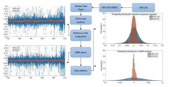
Figure 1.
Orbit determination process.
Figure 1.
Orbit determination process.
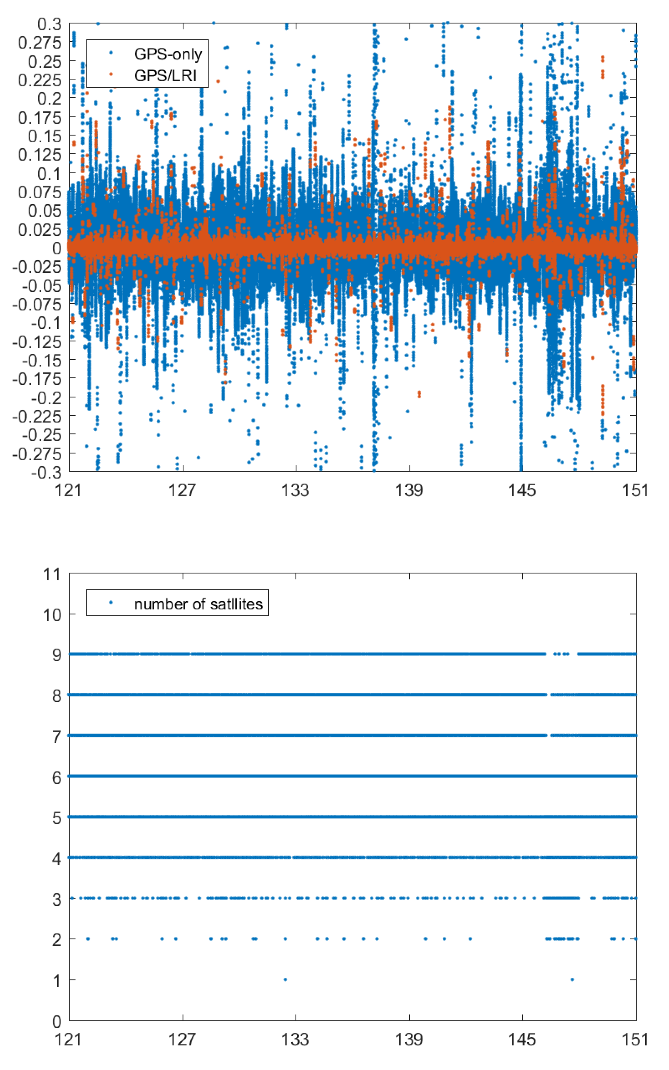
Figure 2.
Reference orbit check for GRACE-FO in the X, Y, Z, 3D (X, Y, Z are components of the baseline vector, unit: m, (a–d)) directions (days 121–151), number of satellites for each epoch (e) and GDOP (f,g).
Figure 2.
Reference orbit check for GRACE-FO in the X, Y, Z, 3D (X, Y, Z are components of the baseline vector, unit: m, (a–d)) directions (days 121–151), number of satellites for each epoch (e) and GDOP (f,g).
Figure 3.
Reference orbit check for GRACE-FO in the X, Y, Z, 3D (X, Y, Z are components of the baseline vector, unit: m, (a–d)) directions (days 151–182), number of satellites for each epoch (e) and GDOP (f,g).
Figure 3.
Reference orbit check for GRACE-FO in the X, Y, Z, 3D (X, Y, Z are components of the baseline vector, unit: m, (a–d)) directions (days 151–182), number of satellites for each epoch (e) and GDOP (f,g).
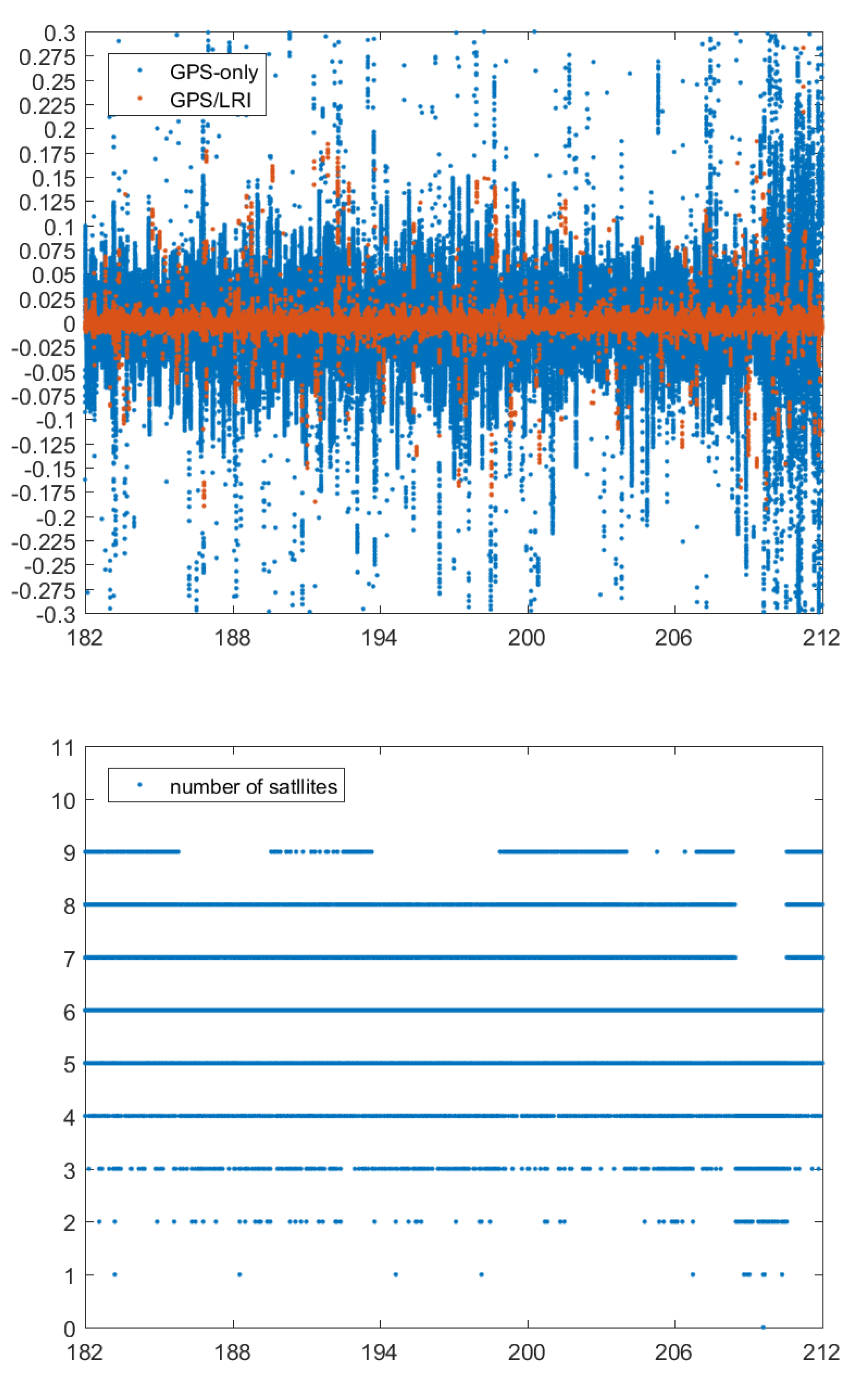
Figure 4.
Reference orbit check for GRACE-FO in the X, Y, Z, 3D (X, Y, Z are components of the baseline vector, unit: m, (a–d)) directions (days 182–212), number of satellites for each epoch (e) and GDOP (f,g).
Figure 4.
Reference orbit check for GRACE-FO in the X, Y, Z, 3D (X, Y, Z are components of the baseline vector, unit: m, (a–d)) directions (days 182–212), number of satellites for each epoch (e) and GDOP (f,g).
Figure 5.
Reference orbit check for GRACE-FO in the X, Y, Z, 3D (X, Y, Z are components of the baseline vector, unit: m, (a–d)) directions (days 212–242), number of satellites for each epoch (e) and GDOP (f,g).
Figure 5.
Reference orbit check for GRACE-FO in the X, Y, Z, 3D (X, Y, Z are components of the baseline vector, unit: m, (a–d)) directions (days 212–242), number of satellites for each epoch (e) and GDOP (f,g).
Figure 6.
Days 121–242 orbit comparison residuals (in the X, Y and Z directions, unit: m) probability distribution for the GPS/LRI and GPS relative orbit.
Figure 6.
Days 121–242 orbit comparison residuals (in the X, Y and Z directions, unit: m) probability distribution for the GPS/LRI and GPS relative orbit.
Figure 7.
Reference orbit check for GRACE-FO-A in the R, S, W, 3D directions (days 121–151, (a–d)).
Figure 7.
Reference orbit check for GRACE-FO-A in the R, S, W, 3D directions (days 121–151, (a–d)).
Figure 8.
Reference orbit check for GRACE-FO-A in the R, S, W, 3D directions (days 151–182, (a–d)).
Figure 8.
Reference orbit check for GRACE-FO-A in the R, S, W, 3D directions (days 151–182, (a–d)).
Figure 9.
Reference orbit check for GRACE-FO-A in the R, S, W, 3D directions (days 182–212, (a–d)).
Figure 9.
Reference orbit check for GRACE-FO-A in the R, S, W, 3D directions (days 182–212, (a–d)).
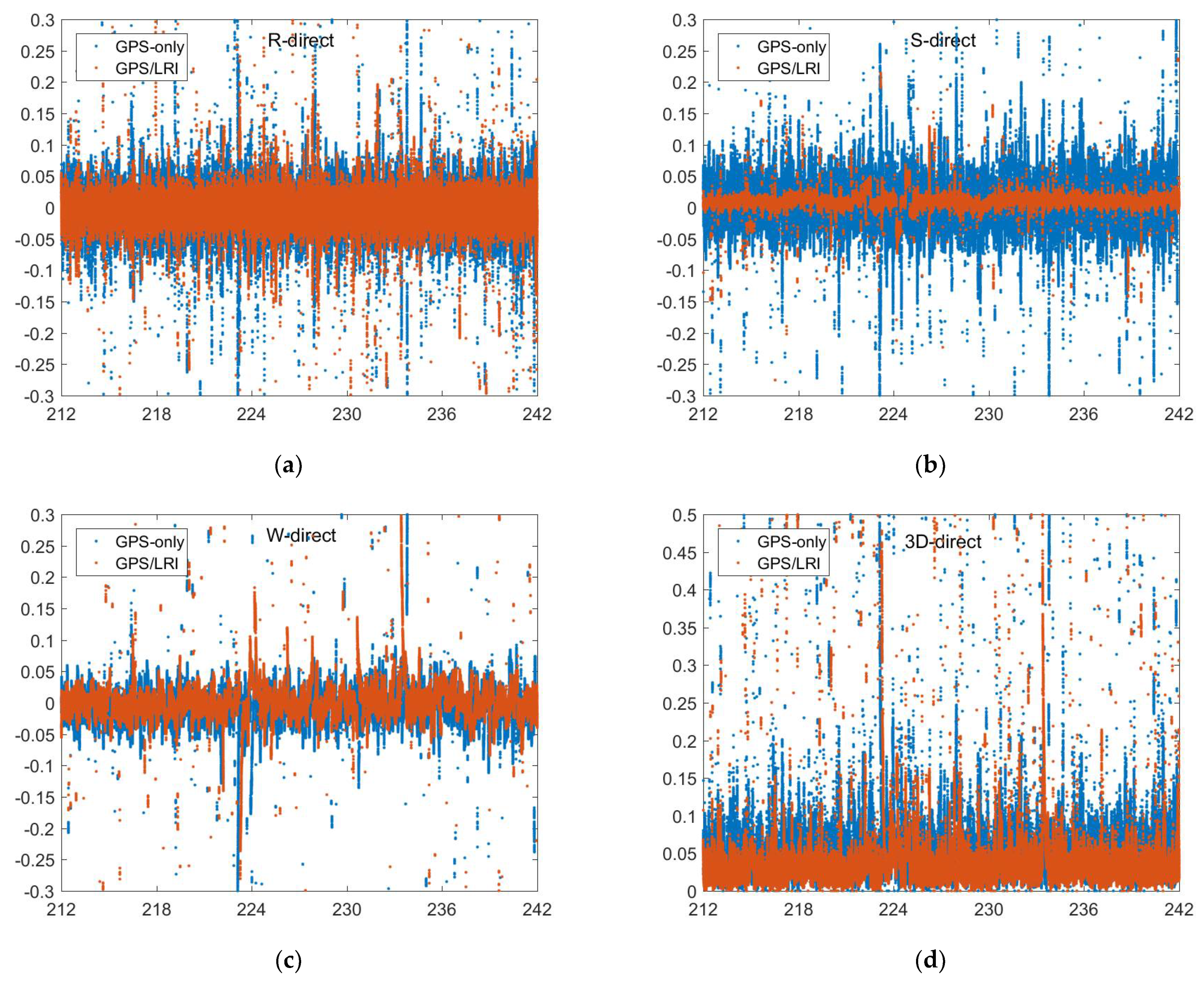
Figure 10.
Reference orbit check for GRACE-FO-A in the R, S, W, 3D directions (days 212–242, (a–d)).
Figure 10.
Reference orbit check for GRACE-FO-A in the R, S, W, 3D directions (days 212–242, (a–d)).
Figure 11.
Days 121–242 orbit comparison residuals (in the R, S and W directions, unit: m) probability distribution for the GPS/LRI and GPS relative orbit.
Figure 11.
Days 121–242 orbit comparison residuals (in the R, S and W directions, unit: m) probability distribution for the GPS/LRI and GPS relative orbit.
Figure 12.
D (X, Y, Z are components of the baseline vector, unit: m, (a–d)) directions (days 121–242).
Figure 12.
D (X, Y, Z are components of the baseline vector, unit: m, (a–d)) directions (days 121–242).
Figure 13.
Eccentricity and eccentricity variation of GRACE-FO satellites (hourly variation).
Figure 13.
Eccentricity and eccentricity variation of GRACE-FO satellites (hourly variation).
Figure 14.
Reference orbit check for Orbital Maneuver in the X, Y, Z, 3D (X, Y, Z are components of the baseline vector, unit: m, (a–d)) directions (days 121–242).
Figure 14.
Reference orbit check for Orbital Maneuver in the X, Y, Z, 3D (X, Y, Z are components of the baseline vector, unit: m, (a–d)) directions (days 121–242).
Figure 15.
Day 121–151 KBR residuals (unit: m) for the GPS/LRI and GPS-only relative orbit and number of satellites.
Figure 15.
Day 121–151 KBR residuals (unit: m) for the GPS/LRI and GPS-only relative orbit and number of satellites.
Figure 16.
Day 151–182 KBR residuals (unit: m) for the GPS/LRI and GPS-only relative orbit and number of satellites.
Figure 16.
Day 151–182 KBR residuals (unit: m) for the GPS/LRI and GPS-only relative orbit and number of satellites.
Figure 17.
Day 182–212 KBR residuals (unit: m) for the GPS/LRI and GPS-only relative orbit and number of satellites.
Figure 17.
Day 182–212 KBR residuals (unit: m) for the GPS/LRI and GPS-only relative orbit and number of satellites.
Figure 18.
Day 213–242 KBR residuals (unit: m) for the GPS/LRI and GPS-only relative orbit and number of satellites.
Figure 18.
Day 213–242 KBR residuals (unit: m) for the GPS/LRI and GPS-only relative orbit and number of satellites.
Figure 19.
Day 121–242 KBR residuals (unit: m) probability distribution for the GPS/LRI and GPS-only relative orbit.
Figure 19.
Day 121–242 KBR residuals (unit: m) probability distribution for the GPS/LRI and GPS-only relative orbit.
Figure 20.
Days 121–242 KBR residuals (unit: m) for the GPS/LRI (a) and GPS-only (b) relative orbit in the Sunlight and Solar eclipse).
Figure 20.
Days 121–242 KBR residuals (unit: m) for the GPS/LRI (a) and GPS-only (b) relative orbit in the Sunlight and Solar eclipse).
Table 1.
RMS of LRI bias (unit: m) and percentage of LRI outliers (unit: %).
Table 1.
RMS of LRI bias (unit: m) and percentage of LRI outliers (unit: %).
| DAY | RMS of LRI Bias | Percentage of LRI Outliers |
|---|
| 121−151 | 0.0492 | 1.21 |
| 151−182 | 0.0480 | 0.73 |
| 182−212 | 0.0535 | 0.98 |
| 212−242 | 0.0544 | 1.85 |
| Average | 0.0513 | 1.19 |
Table 2.
PCO of GRACE-FO satellites (unit: mm).
Table 2.
PCO of GRACE-FO satellites (unit: mm).
| Scheme | Frequency | | PCO | |
|---|
| North | East | Up |
|---|
| GRACE-FO-A | L1 | 1.49 | 0.60 | −7.01 |
| L2 | 0.96 | 0.86 | 22.29 |
| GRACE-FO-B | L1 | 1.49 | 0.60 | −7.01 |
| L2 | 0.96 | 0.86 | 22.29 |
Table 3.
Sensor Offset of GRACE-FO satellites (unit: mm).
Table 3.
Sensor Offset of GRACE-FO satellites (unit: mm).
| Satellite | | Sensor Offset | |
|---|
| North | East | Up |
|---|
| GRACE-FO-A | −261.8 | −0.8 | −531.6 |
| GRACE-FO-B | −260.0 | 0.5 | −530.6 |
Table 4.
Data description.
Table 4.
Data description.
| Data Type | Source | Detail |
|---|
| GPS measurements | GFZ | Sampling rate 1 s; observed values of P1, P2, L1 and L2 |
| LRI measurements | GFZ | Sampling rate 2 s; including observation time and intersatellite distance |
GPS precise ephemeris
GPS precise clock | CODE | Final precise ephemeris; Sampling rate 900 s;
Final precise clock error products;
Sampling rate 30 s |
| Earth rotation parameters | CODE | 121-day values |
| Post-processed science orbit | GFZ | Reduced dynamic orbit |
| K-Band Ranging measurements | GFZ | Sampling rate 5 s |
| Broadcast ephemeris | IGS | BRDC station |
Table 5.
Statistics of reference orbit check (days 121–242) in Earth-fixed coordinate (unit: m).
Table 5.
Statistics of reference orbit check (days 121–242) in Earth-fixed coordinate (unit: m).
| Type | GPS-Only | GPS/LRI |
|---|
| X | Y | Z | 3D | X | Y | Z | 3D |
|---|
| MEAN | 0 | 0.0019 | 0.0017 | − | 0 | 0 | 0.0009 | − |
| MEDIAN | 0 | 0.0025 | 0.0013 | − | 0 | 0.0008 | 0.0012 | − |
| RMS | 0.0378 | 0.0371 | 0.0371 | 0.0676 | 0.0254 | 0.0286 | 0.0219 | 0.0501 |
Table 6.
Statistics of reference orbit check (days 121–242) in RSW (unit: m).
Table 6.
Statistics of reference orbit check (days 121–242) in RSW (unit: m).
| Type | GPS-Only | GPS/LRI |
|---|
| R | S | W | 3D | R | S | W | 3D |
|---|
| MEAN | −0.0010 | 0 | −0.0005 | − | −0.0013 | 0 | 0 | − |
| MEDIAN | −0.0009 | 0 | 0 | − | −0.0008 | 0 | 0 | − |
| RMS | 0.0390 | 0.0406 | 0.0330 | 0.0678 | 0.0290 | 0.0089 | 0.0305 | 0.0500 |
Table 7.
Statistics of X, Y, Z and 3D residual (unit: m, days 121–242) in Sunlight and Solar eclipse.
Table 7.
Statistics of X, Y, Z and 3D residual (unit: m, days 121–242) in Sunlight and Solar eclipse.
| Type | GPS/LRI in Sunlight | GPS/LRI in Solar Eclipse |
|---|
| X | Y | Z | 3D | X | Y | Z | 3D |
|---|
| MEAN | 0 | 0.0007 | −0.0009 | − | 0 | −0.0007 | −0.0009 | − |
| MEDIAN | 0 | 0.0008 | −0.0011 | − | 0 | 0 | −0.0014 | − |
| RMS | 0.0255 | 0.0282 | 0.0216 | 0.0437 | 0.0260 | 0.0302 | 0.0228 | 0.0459 |
Table 8.
Statistics of X, Y, Z and 3D residual (unit: m, days 121–242) in Sunlight and Solar eclipse.
Table 8.
Statistics of X, Y, Z and 3D residual (unit: m, days 121–242) in Sunlight and Solar eclipse.
| Type | GPS-Only in Sunlight | GPS-Only in Solar Eclipse |
|---|
| X | Y | Z | 3D | X | Y | Z | 3D |
|---|
| MEAN | 0.0012 | 0.0018 | 0.0014 | − | 0.0007 | 0.0021 | 0.0023 | − |
| MEDIAN | 0.0007 | 0.0025 | 0.0011 | − | 0 | 0.0022 | 0.0017 | − |
| RMS | 0.0382 | 0.0375 | 0.0374 | 0.0652 | 0.0368 | 0.0362 | 0.0363 | 0.0631 |
Table 9.
Days of Orbital Maneuver.
Table 9.
Days of Orbital Maneuver.
| Circle | Days |
|---|
| red | 135−136 |
| yellow | 149−150 |
| green | 155−156 |
| purple | 163−164 |
| blue | 175−176 |
| black | 230−231 |
Table 10.
Statistics of X, Y, Z and 3D residual (unit: m, days 121–242) in Orbital Maneuver.
Table 10.
Statistics of X, Y, Z and 3D residual (unit: m, days 121–242) in Orbital Maneuver.
| Type | GPS-Only | GPS/LRI |
|---|
| X | Y | Z | 3D | X | Y | Z | 3D |
|---|
| MEAN | −0.0018 | 0 | 0 | − | −0.0010 | 0 | 0 | − |
| MEDIAN | −0.0023 | 0 | 0 | − | −0.0011 | 0 | 0 | − |
| RMS | 0.0367 | 0.0339 | 0.0381 | 0.0604 | 0.0291 | 0.0258 | 0.0228 | 0.0466 |
Table 11.
Statistics of KBR check (unit: m).
Table 11.
Statistics of KBR check (unit: m).
| Day | GPS-Only | GPS\LRI |
|---|
| RMS | MEAN | MEDIAN | RMS | MEAN | MEDIAN |
|---|
| 121–151 | 0.0415 | 0 | 0 | 0.0112 | 0 | −0.0007 |
| 151–182 | 0.0407 | 0 | 0 | 0.0093 | 0 | −0.0006 |
| 182–212 | 0.0458 | 0 | 0 | 0.0086 | 0 | −0.0007 |
| 212–242 | 0.0433 | 0 | 0 | 0.0135 | 0 | −0.0007 |
| Average | 0.0428 | 0 | 0 | 0.0107 | 0 | −0.0007 |
Table 12.
Statistics of KBR residual (unit: m, days 121–242) in Sunlight and Solar eclipse.
Table 12.
Statistics of KBR residual (unit: m, days 121–242) in Sunlight and Solar eclipse.
| Type | GPS/LRI | GPS-Only |
|---|
| Sunlight | Solar Eclipse | Sunlight | Solar Eclipse |
|---|
| MEAN | 0 | 0 | −0.0007 | −0.0006 |
| MEDIAN | 0 | 0.0007 | 0 | 0 |
| RMS | 0.0093 | 0.0097 | 0.0424 | 0.0422 |


 ,
, 


