
Kinematics of Active Landslides in Achaia (Peloponnese, Greece) through InSAR Time Series Analysis and Relation to Rainfall Patterns

 ,
,  , and
, and
Abstract
:1. Introduction
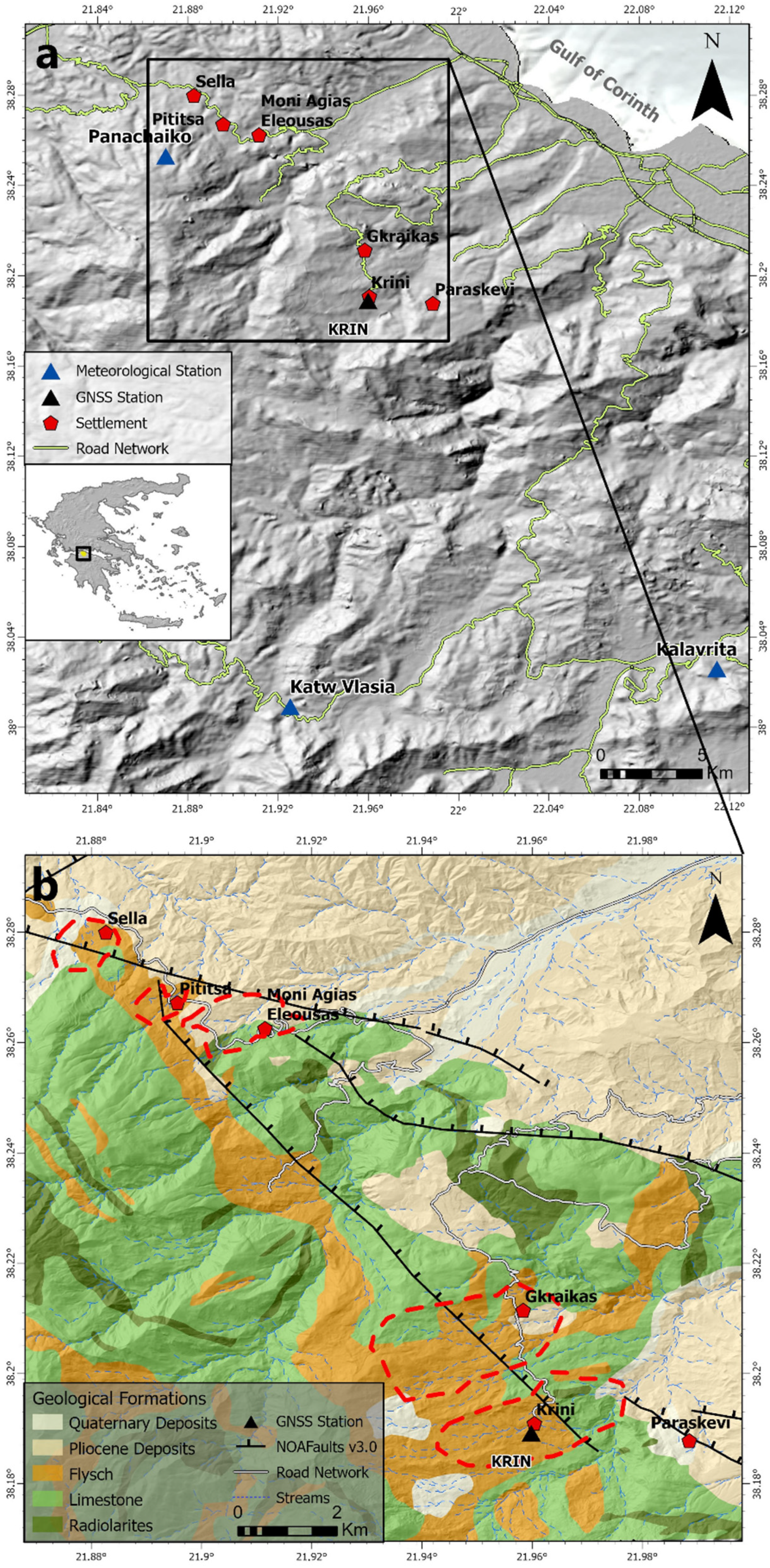
2. Study Area

3. Data, Methods and Results
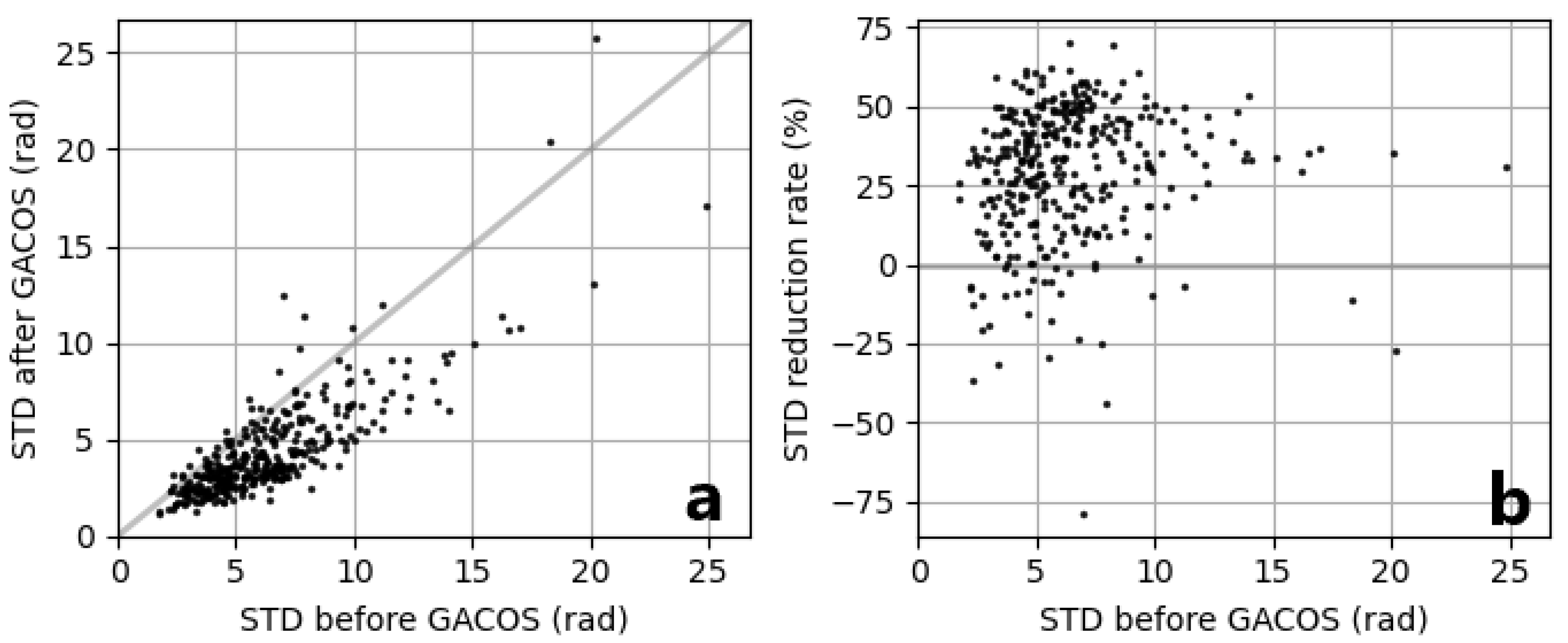
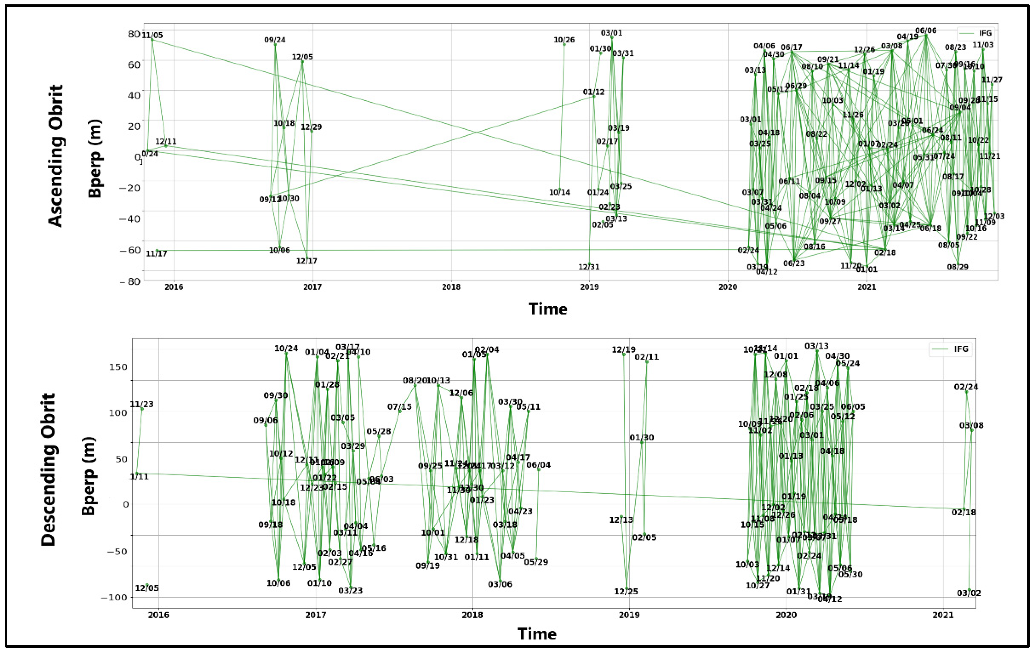
3.1. SAR Data Processing
3.2. Rainfall Data
3.3. Validation of InSAR Time Series with GNSS Data
4. Discussion
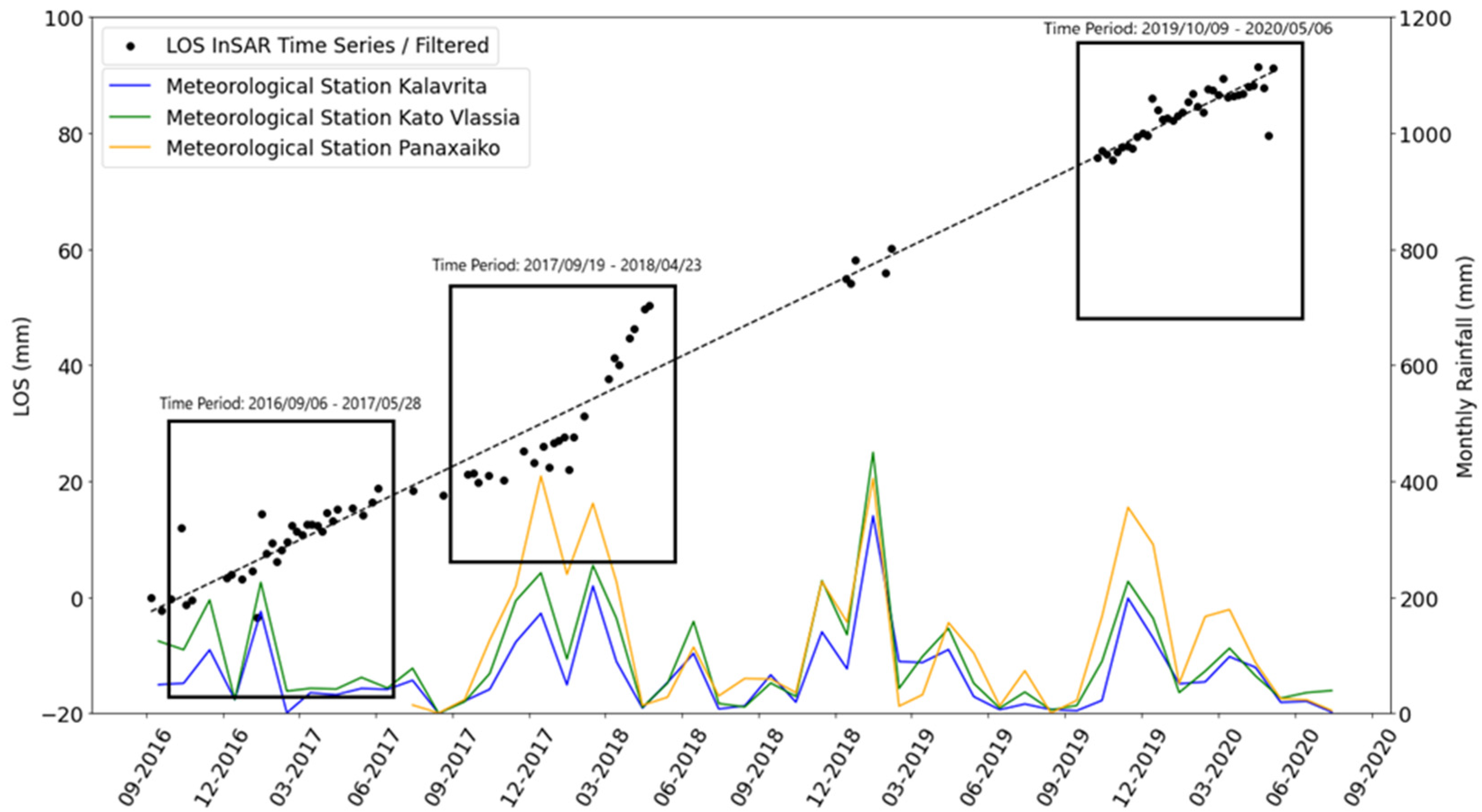
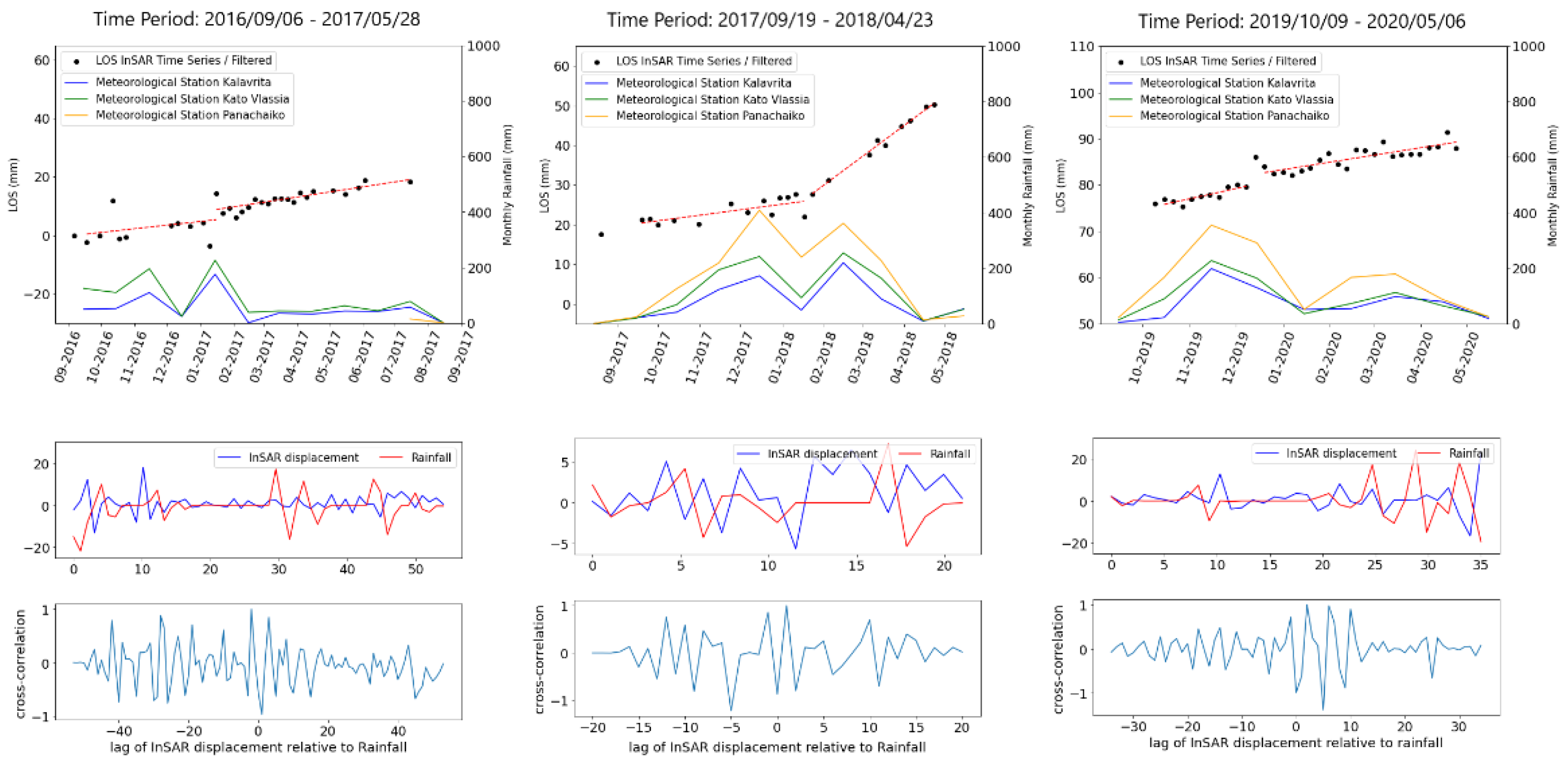
4.1. Landslide Motion and Rainfall Pattern
4.2. Kinematic Characteristics of the Landslides
5. Conclusions
- i.
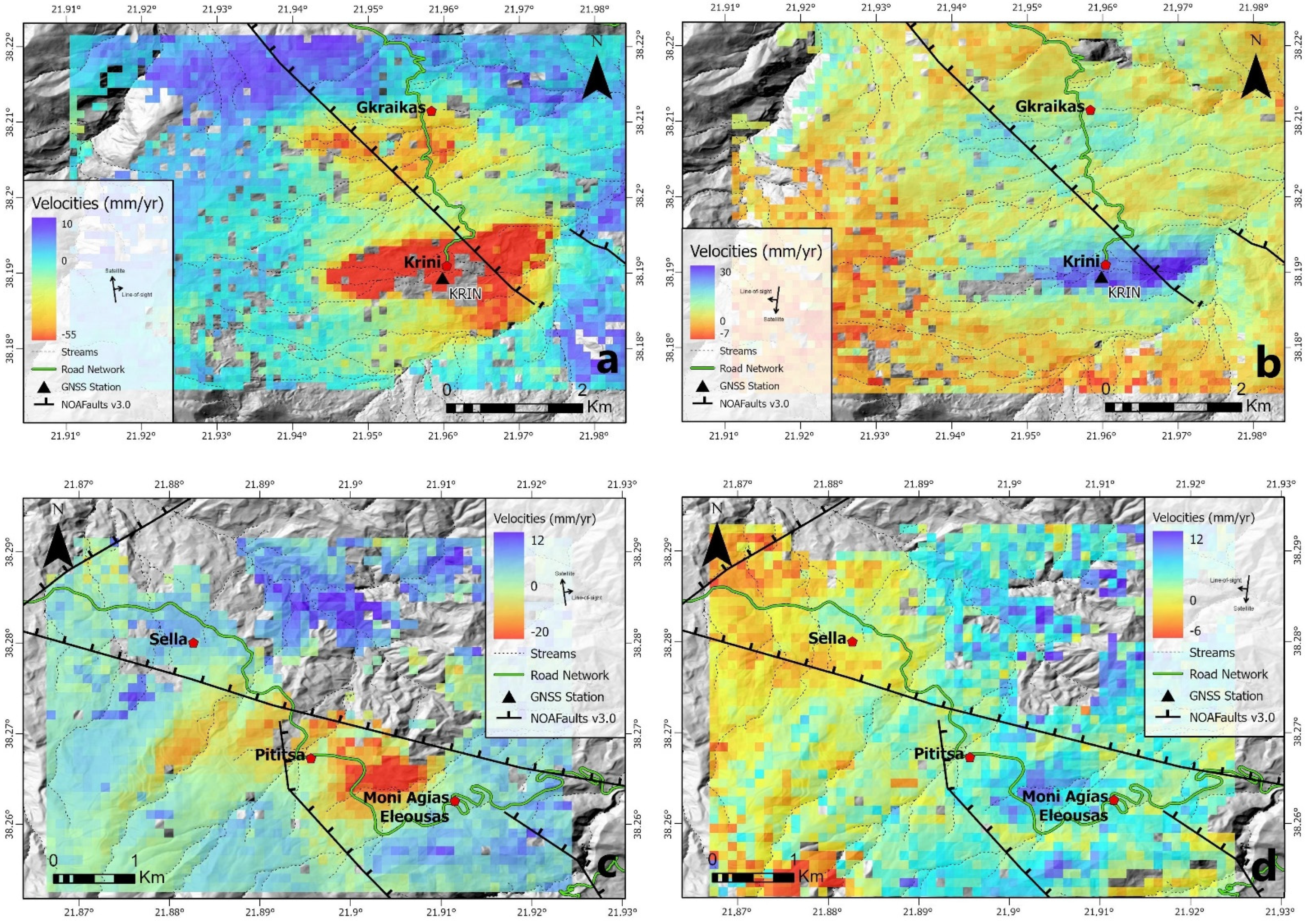
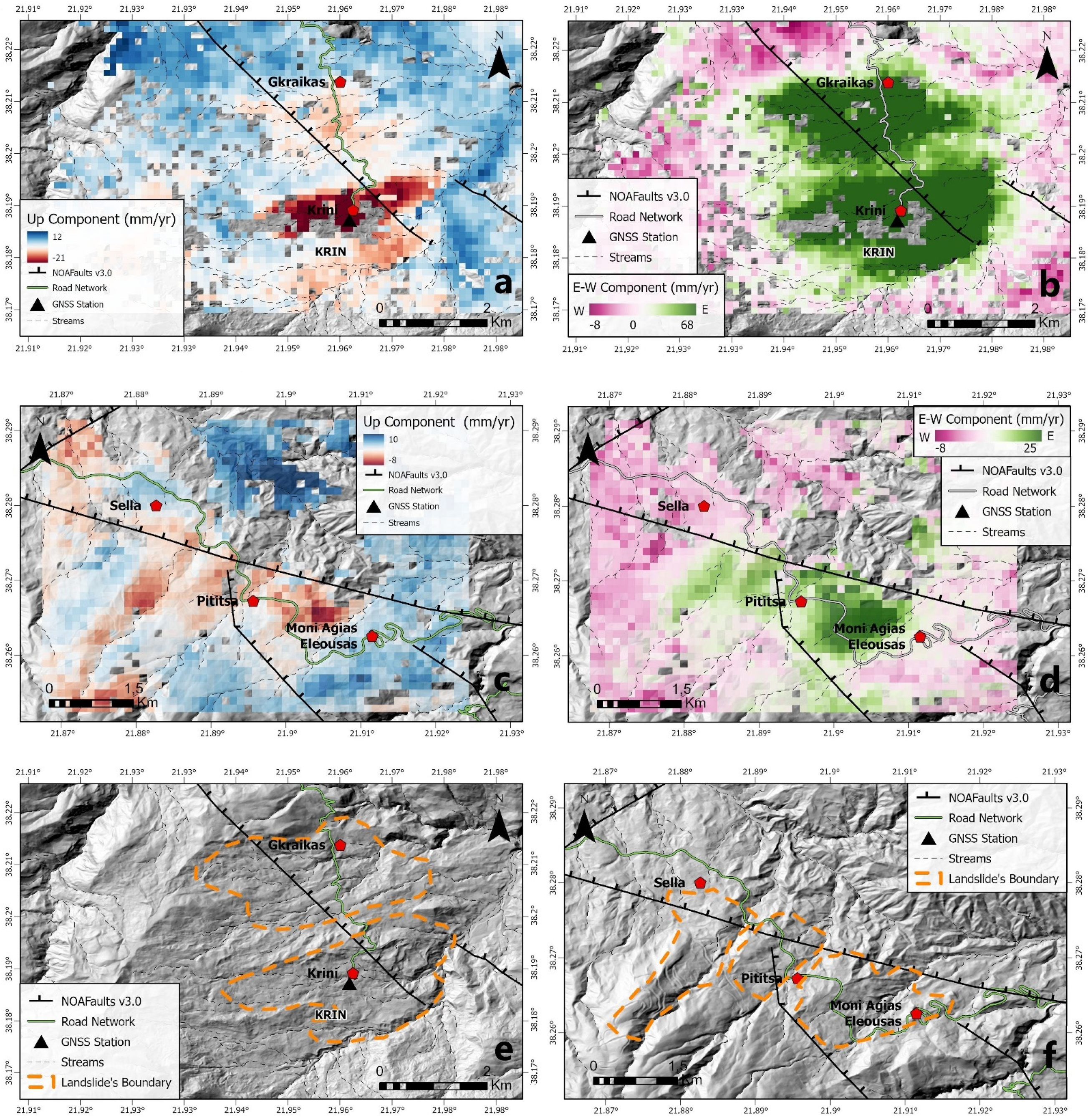
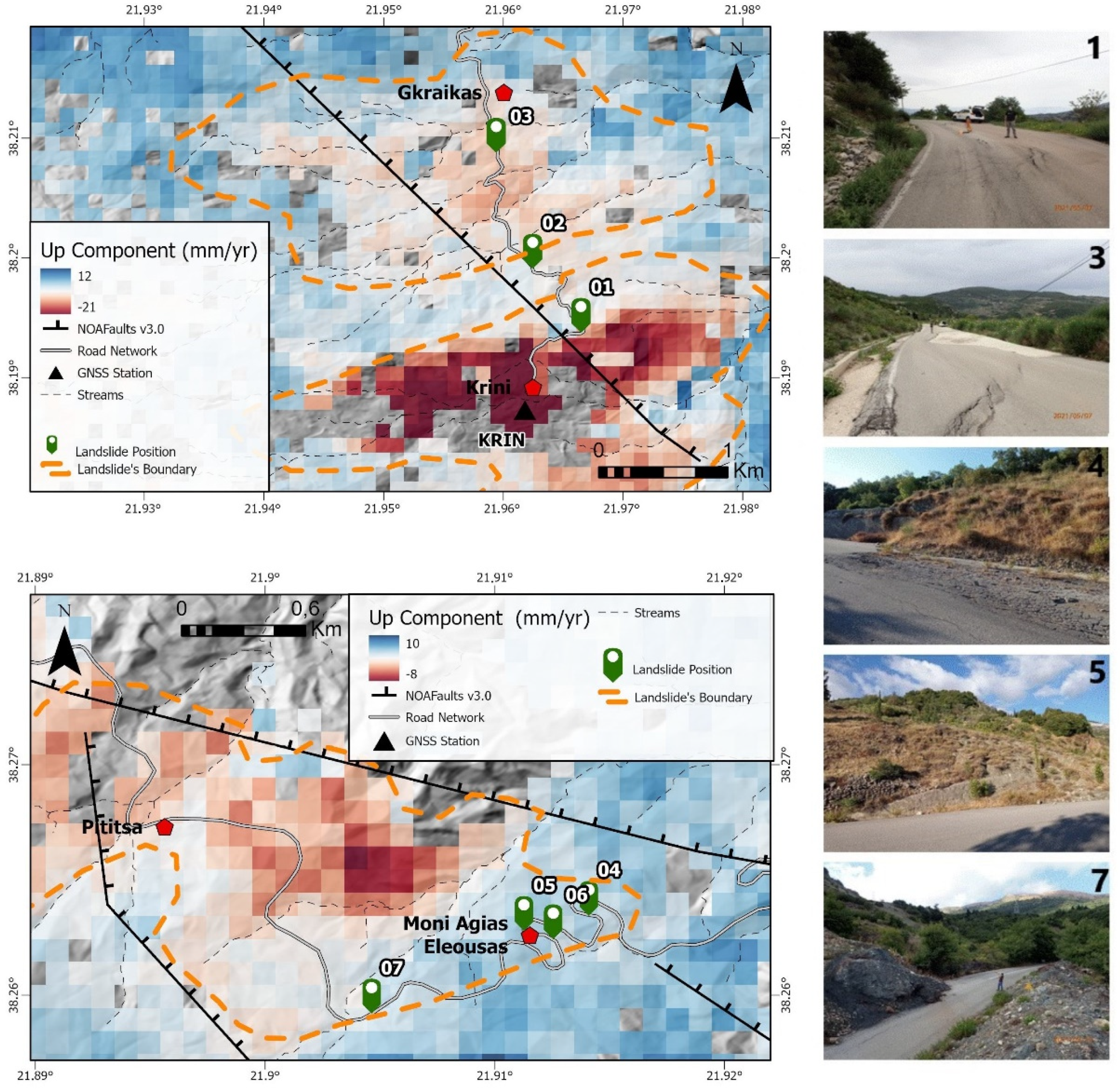
- The Krini, Agia Eleoussa monastery and Pititsa landslides are active landslides whose motion was measured by InSAR (C-band) time series analysis for the period 2016–2021.
- ii.
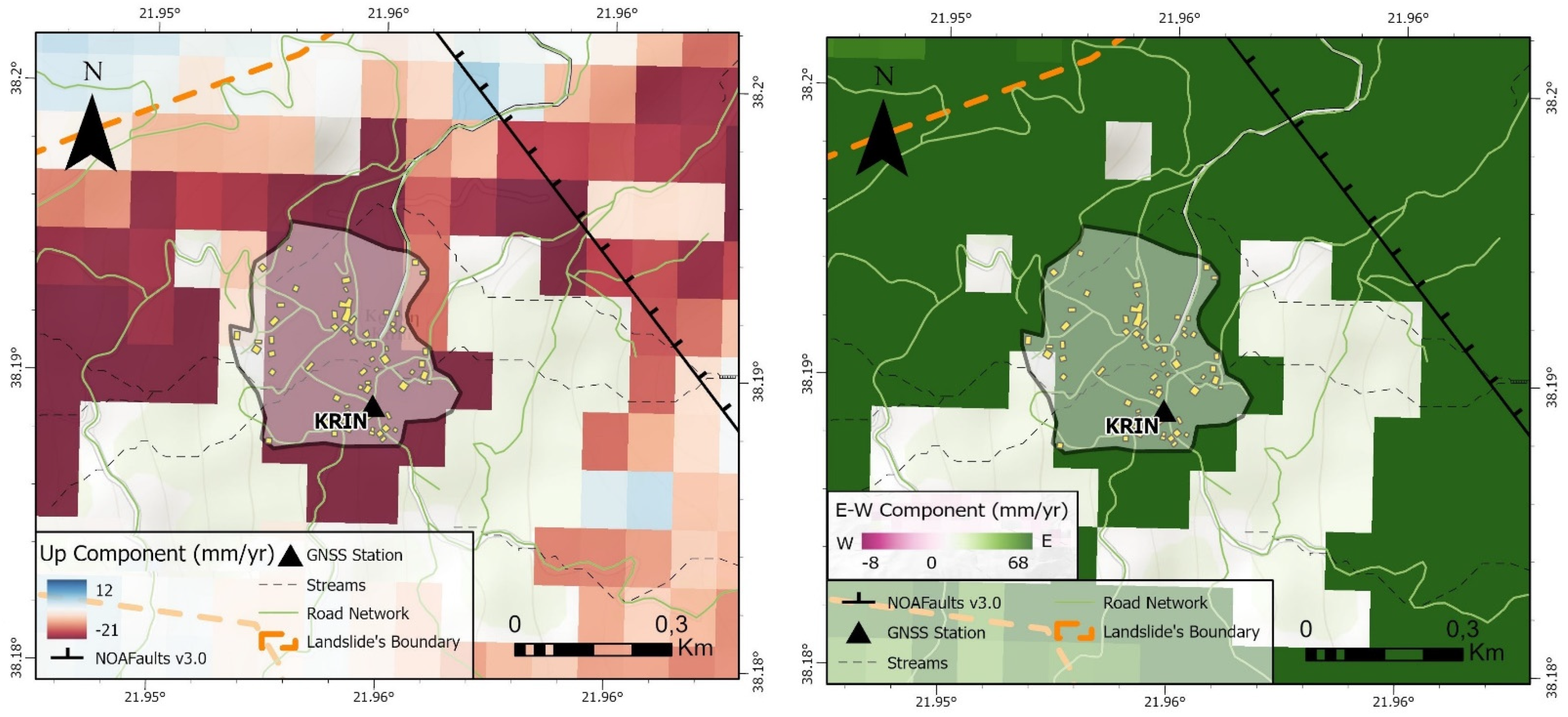
- We processed LiCSAR interferograms using the SBAS tool and we obtained average displacement maps. The results indicate slow ground motions toward the east and downward (subsidence).
- iii.
- The maximum displacement rate of each landslide is located at about the center of each landslide.
- iv.
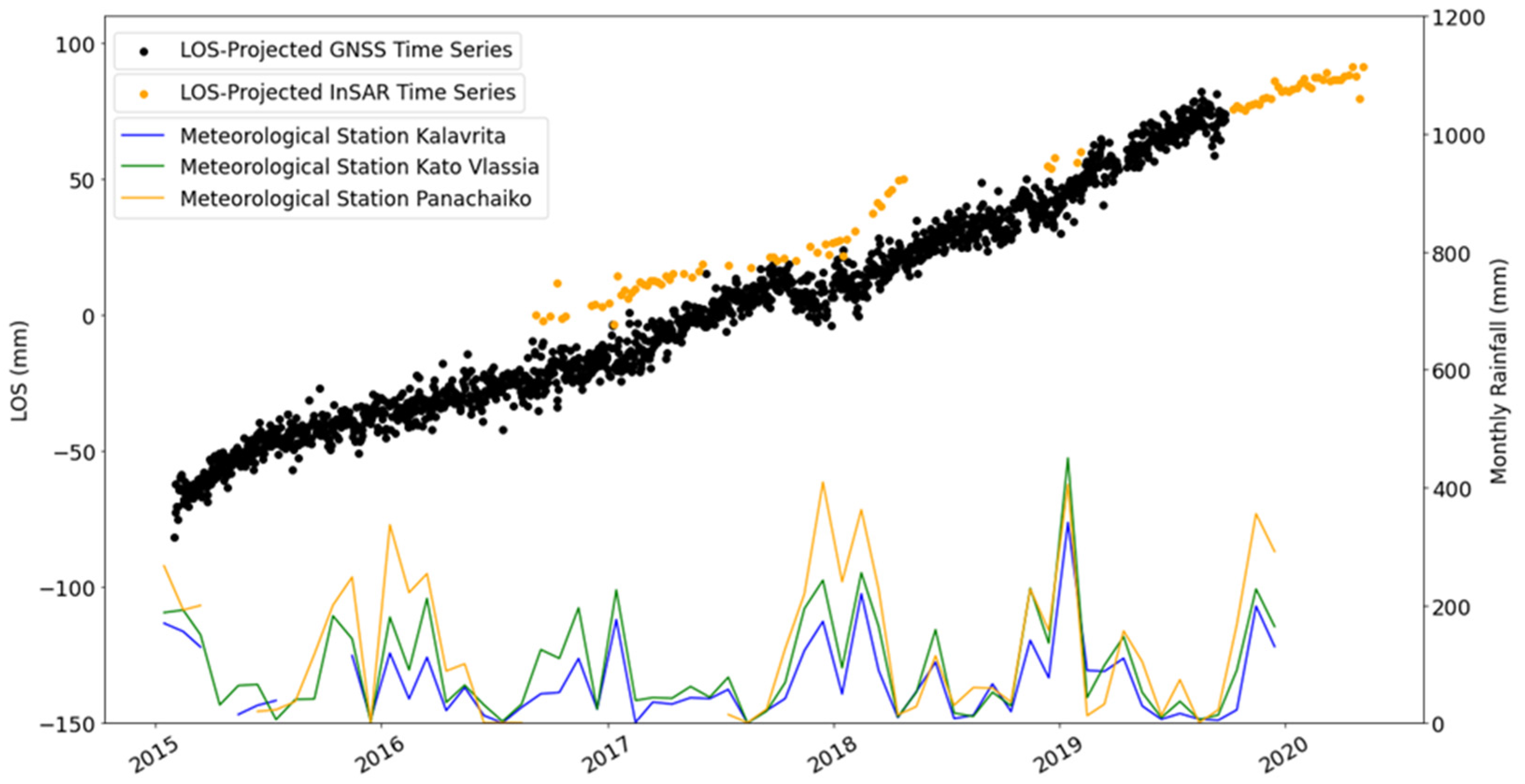
- Our results point that there is a correlation between rainfall and landslide motion. For the Krini landslide, we found the mean time lag to be 13.5 days between the maximum rainfall and the maximum of LOS displacement (descending orbit data).
- v.
- The displacement rates of the Krini active landslide increase after a period of rainfall. Two of the three time periods examined showed an increase in the displacement rate by about 40% when the total rainfall was quite similar (~700 mm). The period September 2017–April 2018 showed an increase in the displacement rate by about 550%. This result was accompanied by a large amount of total rainfall (~1000 mm).
- vi.
- Our findings suggest that the amount of total rainfall could control the amount of increase of the displacement rate of an active landslide.
Supplementary Materials
Author Contributions
Funding
Institutional Review Board Statement
Informed Consent Statement
Data Availability Statement
Acknowledgments
Conflicts of Interest
References
- Colesanti, C.; Wasowski, J. Investigating landslides with space-borne Synthetic Aperture Radar (SAR) interferometry. Eng. Geol. 2006, 88, 173–199. [Google Scholar] [CrossRef]
- Aslan, G.; Foumelis, M.; Raucoules, D.; De Michele, M.; Bernardie, S.; Cakir, Z. Landslide Mapping and Monitoring Using Persistent Scatterer Interferometry (PSI) Technique in the French Alps. Remote Sens. 2020, 12, 1305. [Google Scholar] [CrossRef] [Green Version]
- Solari, L.; Del Soldato, M.; Raspini, F.; Barra, A.; Bianchini, S.; Confuorto, P.; Casagli, N.; Crosetto, M. Review of Satellite Interferometry for Landslide Detection in Italy. Remote Sens. 2020, 12, 1351. [Google Scholar] [CrossRef]
- Kontoes, C.; Loupasakis, C.; Papoutsis, I.; Alatza, S.; Poyiadji, E.; Ganas, A.; Psychogyiou, C.; Kaskara, M.; Antoniadi, S.; Spanou, N. Landslide Susceptibility Mapping of Central and Western Greece, Combining NGI and WoE Methods, with Remote Sensing and Ground Truth Data. Land 2021, 10, 402. [Google Scholar] [CrossRef]
- Elias, P.; Valkaniotis, S.; Ganas, A.; Papathanassiou, G.; Bilia, A.; Kollia, E. Satellite SAR interferometry for monitoring dam deformations: The case of Evinos dam, central Greece. In Proceedings of the Eighth International Conference on Remote Sensing and Geoinformation of the Environment (RSCy2020), Paphos, Cyprus, 16–18 March 2020; Volume 11524, p. 115241I. [Google Scholar] [CrossRef]
- Cruden, D.M.; Varnes, D.J. Landslide Types and Processes, Transportation Research Board. US Natl. Acad. Sci. Spec. Rep. 1996, 247, 36–75. [Google Scholar]
- Singleton, A.; Li, Z.; Hoey, T.; Muller, J.P. Evaluating sub-pixel offset techniques as an alternative to D-InSAR for monitoring episodic landslide movements in vegetated terrain. Remote Sens. Environ. 2014, 147, 133–144. [Google Scholar] [CrossRef] [Green Version]
- Vassilakis, E.; Foumelis, M.; Erkeki, A.; Kotsi, E.; Lekkas, E. Post-event surface deformation of Amyntaio slide (Greece) by complementary analysis of Remotely Piloted Airborne System imagery and SAR interferometry. Appl. Geomat. 2020, 13, 65–75. [Google Scholar] [CrossRef]
- Tsangaratos, P.; Loupasakis, C.; Nikolakopoulos, K.; Angelitsa, V.; Ilia, I. Developing a landslide susceptibility map based on remote sensing, fuzzy logic and expert knowledge of the Island of Lefkada, Greece. Environ. Earth Sci. 2018, 77, 363. [Google Scholar] [CrossRef]
- Kyriou, A.; Nikolakopoulos, K. Assessing the suitability of Sentinel-1 data for landslide mapping. Eur. J. Remote Sens. 2018, 51, 402–411. [Google Scholar] [CrossRef] [Green Version]
- Papoutsis, I.; Kontoes, C.; Alatza, S.; Apostolakis, A.; Loupasakis, C. InSAR Greece with Parallelized Persistent Scatterer Interferometry: A National Ground Motion Service for Big Copernicus Sentinel-1 Data. Remote Sens. 2020, 12, 3207. [Google Scholar] [CrossRef]
- Psychogyiou, C.; Papoutsis, I.; Kontoes, C.; Poyiadji, E.; Spanou, N.; Klimis, N. Multi-temporal Monitoring of slow moving Landslides in south Pindus mountain range, Greece. In Proceedings of the Fringe 2015 Workshop, Frascati, Italy, 23–27 March 2015; pp. 23–27. [Google Scholar]
- Koukis, G.; Sabatakakis, N.; Ferentinou, M.; Lainas, S.; Alexiadou, X.; Panagopoulos, A. Landslide phenomena related to major fault tectonics: Rift zone of Corinth Gulf, Greece. Bull. Eng. Geol. Environ. 2009, 68, 215–229. [Google Scholar] [CrossRef]
- Lebourg, T.; El Bedoui, S.; Hernandez, M. Control of slope deformations in high seismic area: Results from the Gulf of Corinth observatory site (Greece). Eng. Geol. 2009, 108, 295–303. [Google Scholar] [CrossRef]
- Elias, P.; Briole, P. Ground Deformations in the Corinth Rift, Greece, Investigated Through the Means of SAR Multitemporal Interferometry. Geochem. Geophys. Geosystems 2018, 19, 4836–4857. [Google Scholar] [CrossRef] [Green Version]
- Del Soldato, M.; Del Ventisette, C.; Raspini, F.; Righini, G.; Pancioli, V.; Moretti, S. Ground deformation and associated hazards in NW peloponnese (Greece). Eur. J. Remote Sens. 2018, 51, 710–722. [Google Scholar] [CrossRef] [Green Version]
- Chen, W.; Chen, Y.; Tsangaratos, P.; Ilia, I.; Wang, X. Combining Evolutionary Algorithms and Machine Learning Models in Landslide Susceptibility Assessments. Remote Sens. 2020, 12, 3854. [Google Scholar] [CrossRef]
- Sabatakakis, N.; Koukis, G.; Vassiliades, E.; Lainas, S. Landslide susceptibility zonation in Greece. Nat. Hazards 2012, 65, 523–543. [Google Scholar] [CrossRef]
- Papadopoulos, G.A.; Ganas, A.; Koukouvelas, I. Landsliding phenomena in NW Peloponnese, Greece: A test-site of the EC LEWIS research project. Geophys. Res. Abstr. 2006, 8, 04402. [Google Scholar]
- Papathanou, M. Small Scale Displacements within Landslides in the Region of Pititsa Using Earth Surveying and Photogrammetry. Master’s Thesis, University of Patras: Rio-Patras, Greece; 97, (unpublished).
- Katrantsiotis, C. Holocene Environmental Changes and Climate Variability in the Eastern Mediterranean: Multiproxy Sediment Records from the Peloponnese Peninsula, SW Greece. Ph.D. Thesis, Department of Physical Geography, Stockholm University, Stockholm, Sweden, 2019. [Google Scholar]
- Bernard, P.; Lyon-Caen, H.; Briole, P.; Deschamps, A.; Boudin, F.; Makropoulos, K.; Papadimitriou, P.; Lemeille, F.; Patau, G.; Billiris, H.; et al. Seismicity, deformation and seismic hazard in the western rift of Corinth: New insights from the Corinth Rift Laboratory (CRL). Tectonophysics 2006, 426, 7–30. [Google Scholar] [CrossRef]
- Clarke, P.J.; Davies, R.R.; England, P.C.; Parsons, B.; Billiris, H.; Paradissis, D.; Veis, G.; Cross, P.A.; Denys, P.H.; Ashkenazi, V.; et al. Crustal strain in central Greece from repeated GPS measurements in the interval 1989-1997. Geophys. J. Int. 1998, 135, 195–214. [Google Scholar] [CrossRef] [Green Version]
- Chousianitis, K.; Ganas, A.; Evangelidis, C.P. Strain and rotation rate patterns of mainland Greece from continuous GPS data and comparison between seismic and geodetic moment release. J. Geophys. Res. Solid Earth 2015, 120, 3909–3931. [Google Scholar] [CrossRef]
- Briole, P.; Ganas, A.; Elias, P.; Dimitrov, D. The GPS velocity field of the Aegean. New observations, contribution of the earthquakes, crustal blocks model. Geophys. J. Int. 2021, 226, 468–492. [Google Scholar] [CrossRef]
- Elias, P.; Kontoes, C.; Papoutsis, I.; Kotsis, I.; Marinou, A.; Paradissis, D.; Sakellariou, D. Permanent Scatterer InSAR Analysis and Validation in the Gulf of Corinth. Sensors 2009, 9, 46–55. [Google Scholar] [CrossRef] [Green Version]
- Trikolas, C.; Koskeridou, E.; Tsourou, T.; Drinia, H.; Alexouli-Livaditi, A. Pleistocene marine deposits of the Aigialia region (N. Peloponnesus). Bull. Geol. Soc. Greece 2004, 36, 826–835. [Google Scholar] [CrossRef] [Green Version]
- Palyvos, N.; Sorel, D.; Lemeille, F.; Mancini, M.; Pantosti, D.; Julià, R.; Triantaphyllou, M.; De Martini, P.M. Review and New Data on Uplift Rates at the W Termination of the Corinth Rift and the Ne Rion Graben Area (Achaia, Nw Peloponnesos). Bull. Geol. Soc. Greece 2018, 40, 412–424. [Google Scholar] [CrossRef] [Green Version]
- Avallone, A.; Briole, P.; Agatza-Balodimou, A.M.; Billiris, H.; Charade, O.; Mitsakaki, C.; Nercessian, A.; Papazissi, K.; Paradissis, D.; Veis, G. Analysis of eleven years of deformation measured by GPS in the Corinth Rift Laboratory area. Comptes Rendus Geosci. 2004, 336, 301–311. [Google Scholar] [CrossRef] [Green Version]
- Roberts, P.G.; Koukouvelas, I. Structural and seismological segmentation of the Gulf of Corinth fault system: Implications for models of fault growth. Ann. Geofis. 1996, 39, 619–646. [Google Scholar]
- Roberts, G.; Ganas, A. Fault-slip directions in central and southern Greece measured from striated and corrugated fault planes: Comparison with focal mechanism and geodetic data. J. Geophys. Res. Earth Surf. 2000, 105, 23443–23462. [Google Scholar] [CrossRef]
- Koukouvelas, I.; Stamatopoulos, L.; Katsonopoulou, D.; Pavlides, S. A paleoseismological and geoarchaeological investigation of Eliki fault, Gulf of Corinth, Greece. J. Struct. Geol. 2001, 23, 531–543. [Google Scholar] [CrossRef]
- Verrios, S.; Zygouri, V.; Kokkalas, S. MORPHOTECTONIC ANALYSIS IN THE ELIKI FAULT ZONE (GULF OF CORINTH, GREECE). Bull. Geol. Soc. Greece 2004, 36, 1706–1715. [Google Scholar] [CrossRef] [Green Version]
- Palyvos, N.; Pantosti, D.; De Martini, P.M.; Lemeille, F.; Sorel, D.; Pavlopoulos, K. The Aigion-Neos Erineos coastal normal fault system (western Corinth Gulf Rift, Greece): Geomorphological signature, recent earthquake history, and evolution. J. Geophys. Res. Earth Surf. 2005, 110, B09302. [Google Scholar] [CrossRef] [Green Version]
- Tsimi, C.; Ganas, A.; Soulakellis, N.; Kairis, O.; Valmis, S. MORPHOTECTONICS OF THE PSATHOPYRGOS ACTIVE FAULT, WESTERN CORINTH RIFT, CENTRAL GREECE. Bull. Geol. Soc. Greece 2018, 40, 500–511. [Google Scholar] [CrossRef] [Green Version]
- Verroios, S.; Zygouri, V. Geomorphological Analysis of Xilokastro Fault, Central Gulf of Corinth, Greece. Geosciences 2021, 11, 516. [Google Scholar] [CrossRef]
- Zygouri, V.; Koukouvelas, I.K. Landslides and natural dams in the Krathis River, north Peloponnese, Greece. Bull. Eng. Geol. Environ. 2019, 78, 207–222. [Google Scholar] [CrossRef]
- Rozos, D.; Bathrellos, D.; Skilodimou, D. Landslide Susceptibility Mapping of the northeastern part of Achaia Prefecture using analytical hierarchical process and GIS techniques. Bull. Geol. Soc. Greece 2010, 43, 1637–1646. [Google Scholar] [CrossRef] [Green Version]
- Rozos, D.; Bathrellos, G.D.; Skillodimou, H.D. Comparison of the implementation of rock engineering system and analytic hierarchy process methods, upon landslide susceptibility mapping, using GIS: A case study from the Eastern Achaia County of Peloponnesus, Greece. Environ. Earth Sci. 2010, 63, 49–63. [Google Scholar] [CrossRef]
- Kavoura, K. Landslide Inventory Map Using GIS Tools and Field Experience—The Case of Achaia Prefecture, Western Greece. Master’s Thesis, University of Patras, Rio-Patra, Greece, 2013; p. 98. [Google Scholar]
- Polykretis, C.; Ferentinou, M.; Chalkias, C. A comparative study of landslide susceptibility mapping using landslide susceptibility index and artificial neural networks in the Krios River and Krathis River catchments (northern Peloponnesus, Greece). Bull. Eng. Geol. Environ. 2015, 74, 27–45. [Google Scholar] [CrossRef]
- Konstantopoulos, K.; Miliaresis, G.C.; Desk, S. Unsupervised landslide risk dependent terrain segmentation on the basis of historical landslide data and geomorphometrical indicators. SDRP J. Earth Sci. Environ. Stud. 2018, 3, 1–9. [Google Scholar] [CrossRef] [Green Version]
- Tsangaratos, P.; Loupasakis, C.; Rozos, D.; Ilia, I. Landslide susceptibility assessments using the k-Nearest Neighbor algo-rithm and expert knowledge. Case study of the basin of Selinounda River 2015, Achaia County, Greece. In Proceedings of the SafeChania 2015. The Knowledge Triangle in the Civil Protection Service Center of Mediterranean Architecture, Chania, Greece, 10–14 June 2015; pp. 10–14. [Google Scholar]
- Sabatakakis, N.; Tsiambaos, G.; Rondoyanni, T.; Papanakli, S.; Kavoura, K. Deep-Seated Structurally Controlled Landslides of Corinth Gulf Rift Zone, Greece: The Case of Panagopoula Landslide. In Proceedings of the 13th ISRM International Congress of Rock Mechanics, Montreal, QC, Canada, 10–13 May 2015; Paper Number: ISRM-13CONGRESS-2015-273. ISBN 978-1-926872-25-4. [Google Scholar]
- Guzzetti, F.; Ardizzone, F.; Cardinali, M.; Rossi, M.; Valigi, D. Landslide volumes and landslide mobilization rates in Umbria, central Italy. Earth Planet. Sci. Lett. 2009, 279, 222–229. [Google Scholar] [CrossRef]
- Tavoularis, N.; Papathanassiou, G.; Ganas, A.; Argyrakis, P. Development of the Landslide Susceptibility Map of Attica Region, Greece, Based on the Method of Rock Engineering System. Land 2021, 10, 148. [Google Scholar] [CrossRef]
- Loftus, D.L.; Tsoflias, P. Geological Map of Greece in scale 1:50000. NAFPAKTOS Map Sheet; Institute of Geology and Mineral Exploration: Athens, Greece, 1971. [Google Scholar]
- Tsoflias, P. Geological Map of Greece in scale 1:50000. KHALANDRITSA Map Sheet; Institute of Geology and Mineral Exploration: Athens, Greece, 1984. [Google Scholar]
- Eleftheriou, A. Geotechnical Report on the Areas of Elekistra–Argyra and Krini Villages of the Achaia District; IGME: Athens, Greece, 1985; p. 13. [Google Scholar]
- Varnes, D.J. Slope movement types and processes. Spec. Rep. 1978, 176, 11–33. [Google Scholar]
- Hungr, O.; Leroueil, S.; Picarelli, L. The Varnes classification of landslide types, an update. Landslides 2014, 11, 167–194. [Google Scholar] [CrossRef]
- Bertolini, G.; Guida, M.; Pizziolo, M. Landslides in Emilia-Romagna region (Italy): Strategies for hazard assessment and risk management. Landslides 2005, 2, 302–312. [Google Scholar] [CrossRef]
- Morishita, Y.; Lazecky, M.; Wright, T.J.; Weiss, J.R.; Elliott, J.R.; Hooper, A. LiCSBAS: An Open-Source InSAR Time Series Analysis Package Integrated with the LiCSAR Automated Sentinel-1 InSAR Processor. Remote Sens. 2020, 12, 424. [Google Scholar] [CrossRef] [Green Version]
- COMET-LiCS Sentinel-1 InSAR Portal. Available online: https://comet.nerc.ac.uk/COMET-LiCS-portal/ (accessed on 26 May 2021).
- LiCSBAS: LiCSBAS Package to Conduct InSAR Time Series Analysis Using LiCSAR Products. Available online: https://github.com/yumorishita/LiCSBAS (accessed on 26 May 2021).
- Werner, C.; Wegmüller, U.; Strozzi, T.; Wiesmann, A. Gamma SAR and interferometric processing software. In Proceedings of the ERS-ENVISAT Symposium 2000, Gothenburg, Sweden, 16–20 October 2000. [Google Scholar]
- Wegmüller, U.; Werner, C.; Strozzi, T.; Wiesmann, A.; Frey, O.; Santoro, M. Sentinel-1 IWS mode support in the GAMMA software. In Proceedings of the 2015 IEEE 5th Asia-Pacific Conference on Synthetic Aperture Radar (APSAR), Singapore, 1–4 September 2015. [Google Scholar]
- Chen, C.W.; Zebker, H.A. Phase unwrapping for large SAR interferograms: Statistical segmentation and generalized network models. IEEE Trans. Geosci. Remote Sens. 2002, 40, 1709–1719. [Google Scholar] [CrossRef] [Green Version]
- Wang, Q.; Yu, W.; Xu, B.; Wei, G. Assessing the use of GACOS products for SBAS-INSAR deformation monitoring: A case in Southern California. Sensors 2019, 19, 3894. [Google Scholar] [CrossRef]
- Biggs, J.; Wright, T.; Lu, Z.; Parsons, B. Multi-interferogram method for measuring interseismic deformation: Denali Fault, Alaska. Geophys. J. Int. 2007, 170, 1165–1179. [Google Scholar] [CrossRef] [Green Version]
- López-Quiroz, P.; Doin, M.P.; Tupin, F.; Briole, P.; Nicolas, J.M. Time series analysis of Mexico City subsidence constrained by radar interferometry. J. Appl. Geophys. 2009, 69, 1–15. [Google Scholar] [CrossRef]
- Wright, T.J.; Parsons, B.E.; Lu, Z. Toward mapping surface deformation in three dimensions using InSAR. Geophys. Res. Lett. 2004, 31, L01607. [Google Scholar] [CrossRef] [Green Version]
- Motagh, M.; Shamshiri, R.; Haghshenas-Haghighi, M.; Wetzel, H.-U.; Akbari, B.; Nahavandchi, H.; Roessner, S.; Arabi, S. Quantifying groundwater exploitation induced subsidence in the Rafsanjan plain, southeastern Iran, using InSAR time-series and in situ measurements. Eng. Geol. 2017, 218, 134–151. [Google Scholar] [CrossRef]
- Lagouvardos, K.; Kotroni, V.; Bezes, A.; Koletsis, I.; Kopania, T.; Lykoudis, S.; Mazarakis, N.; Papagiannaki, K.; Vougioukas, S. The automatic weather stations NOANN network of the National Observatory of Athens: Operation and database. Geosci. Data J. 2017, 4, 4–16. [Google Scholar] [CrossRef]
- Guzzetti, F.; Peruccacci, S.; Rossi, M.; Stark, C.P. Rainfall thresholds for the initiation of landslides in central and southern Europe. Meteorol. Atmos. Phys. 2007, 98, 239–267. [Google Scholar] [CrossRef]
- Guzzetti, F.; Peruccacci, S.; Rossi, M.; Stark, C.P. The rainfall intensity–duration control of shallow landslides and debris flows: An update. Landslides 2008, 5, 3–17. [Google Scholar] [CrossRef]
- Segoni, S.; Piciullo, L.; Gariano, S.L. A review of the recent literature on rainfall thresholds for landslide occurrence. Landslides 2018, 15, 1483–1501. [Google Scholar] [CrossRef]
- Wei, Z.-L.; Shang, Y.-Q.; Sun, H.-Y.; Xu, H.-D.; Wang, D.-F. The effectiveness of a drainage tunnel in increasing the rainfall threshold of a deep-seated landslide. Landslides 2019, 16, 1731–1744. [Google Scholar] [CrossRef]
- Tomás, R.; Li, Z.; Lopez-Sanchez, J.M.; Liu, P.; Singleton, A. Using wavelet tools to analyse seasonal variations from InSAR time-series data: A case study of the Huangtupo landslide. Landslides 2015, 13, 437–450. [Google Scholar] [CrossRef] [Green Version]
- Bracewell, R. Pentagram Notation for Cross Correlation. The Fourier Transform and Its Applications; McGraw-Hill: New York, NY, USA, 1965; pp. 46, 243. [Google Scholar]
- Ganas, A. NOAFAULTS KMZ Layer Version 3.0 (2020 Update) (Version V3.0) [Data Set]. Zenodo 2020. [Google Scholar] [CrossRef]
- Ganas, A.; Tsironi, V.; Kollia, E.; Delagas, M.; Tsimi, C.; Oikonomou, A. Recent upgrades of the NOA database of active faults in Greece (NOAFAULTs). In Proceedings of the 19th General Assembly of WEGENER, Grenoble, France, 10–13 September 2018; pp. 10–13. [Google Scholar]
- Natijne, A.L.; Lindenbergh, R.C.; Bogaard, T.A. Machine Learning: New Potential for Local and Regional Deep-Seated Landslide Nowcasting. Sensors 2020, 20, 1425. [Google Scholar] [CrossRef] [Green Version]
- Villaseñor-Reyes, C.I.; Dávila-Harris, P.; Delgado-Rodríguez, O. Multidisciplinary approach for the characterization of a deep-seated landslide in a semi-arid region (Cañón de Yerbabuena, San Luis Potosí, Mexico). Landslides 2021, 18, 367–381. [Google Scholar] [CrossRef]


| Mean Velocity (mm/yr) | Median Velocity (mm/yr) | |
|---|---|---|
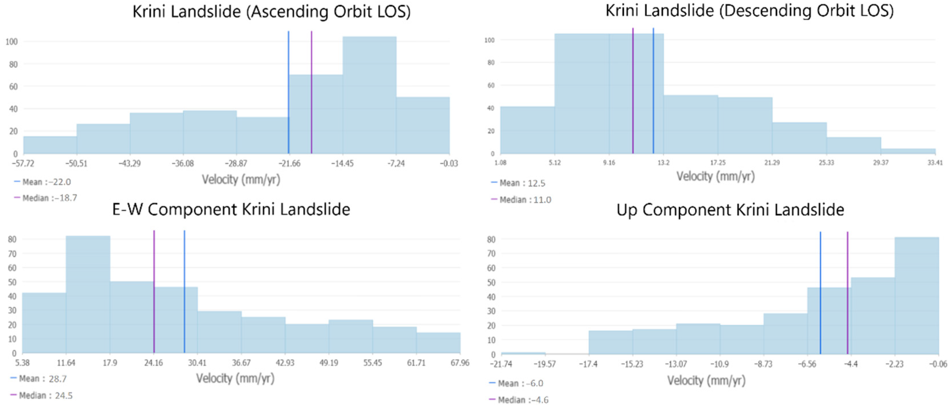
| Krini Up Component | −6.0 | −4.6 |
| Krini E-W Component | 28.7 | 24.5 |
| Krini LOS (ascending) | −22.0 | −18.7 |
| Krini LOS (descending) | 12.5 | 11.0 |
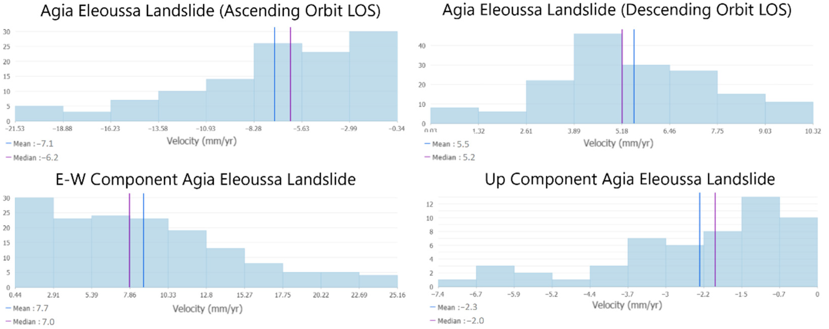
| Agia Eleoussa Up Component | −1.8 | −1.2 |
| Agia Eleoussa E-W Component | 7.7 | 7.0 |
| Agia Eleoussa LOS (ascending) | −7.1 | −6.3 |
| Agia Eleoussa LOS (descending) | 5.5 | 5.2 |
| Time Period of Time Series | Displacement Rates A (mm/yr) | Displacement Rates B (mm/yr) | Total Rainfall (mm) (Kato Vlassia Station) | Time Lag between Rainfall Peak and InSAR Time Series (Days) |
|---|---|---|---|---|
| 6 September 2016–28 May 2017 | 14.8 | 20.8 | 712 | 17.6 |
| 19 September 2017–23 April 2018 | 16.6 | 92.6 | 1041 | 12 |
| 9 October 2019–6 May 2020 | 19.1 | 26.6 | 704 | 11 |
| 24 September 2020–31 May 2021 | 30.0 | 99.8 | 935 | 12 |
Publisher’s Note: MDPI stays neutral with regard to jurisdictional claims in published maps and institutional affiliations. |
© 2022 by the authors. Licensee MDPI, Basel, Switzerland. This article is an open access article distributed under the terms and conditions of the Creative Commons Attribution (CC BY) license (https://creativecommons.org/licenses/by/4.0/).
Share and Cite
Tsironi, V.; Ganas, A.; Karamitros, I.; Efstathiou, E.; Koukouvelas, I.; Sokos, E. Kinematics of Active Landslides in Achaia (Peloponnese, Greece) through InSAR Time Series Analysis and Relation to Rainfall Patterns. Remote Sens. 2022, 14, 844. https://doi.org/10.3390/rs14040844
Tsironi V, Ganas A, Karamitros I, Efstathiou E, Koukouvelas I, Sokos E. Kinematics of Active Landslides in Achaia (Peloponnese, Greece) through InSAR Time Series Analysis and Relation to Rainfall Patterns. Remote Sensing. 2022; 14(4):844. https://doi.org/10.3390/rs14040844
Chicago/Turabian StyleTsironi, Varvara, Athanassios Ganas, Ioannis Karamitros, Eirini Efstathiou, Ioannis Koukouvelas, and Efthimios Sokos. 2022. "Kinematics of Active Landslides in Achaia (Peloponnese, Greece) through InSAR Time Series Analysis and Relation to Rainfall Patterns" Remote Sensing 14, no. 4: 844. https://doi.org/10.3390/rs14040844