1. Introduction
In the context of global warming, great efforts have been made to investigate surface energy balance (SEB) at the Antarctic Ice Sheet, because it is a crucial factor affecting the surface mass balance that could either mitigate or exacerbate the global sea level rise [
1,
2]. On the Antarctic Ice Sheet, the surface energy flux is an important input variable for the verification of climate models, and the air temperature can influence the surface characteristics, such as albedo, limiting the absorption of the shortwave radiation and emission of longwave radiation [
3,
4]. Given the ecological significance of air temperature, acquiring real-time air temperature on the Antarctic Ice Sheet is vital to the surface energy budget. However, due to the extreme weather in the Antarctic, in situ meteorological observation has been sparse, and reanalysis products, such as ERA-40,NCEP, and JRA-25, suffer from large uncertainties [
5]. Although air temperature is very easily observed from satellite sensors, larger errors exist very close to the surface and in extreme conditions, and the ice surface temperature can be retrieved with a bias of 2 K [
6]. According to its close correlation with the ice surface temperature, the air temperature could be estimated based on thermodynamic mechanisms and statistical patterns.
Air temperature simulations have become an important application area of machine learning. Artificial neural network and random forests are relatively widely used in methods for obtaining air temperature products from remote sensing images of surface temperatures and have been developed and progressed in most parts of the Earth. However, in fact, air temperature estimations from remotely sensed land surface temperatures are far from straightforward [
7,
8]. The difference between land surface temperature and air temperature is strongly influenced by surface characteristics and atmospheric conditions [
9,
10]. However, machine learning has a strong ability to solve nonlinear relation fitting. Meyer et al. [
11] took MSG SEVIRI channel information, the NDVI, altitude, and solar zenith angle as the input of a random forest model and adjusted the parameters by using 10-fold “leave-location-and-time-out” cross-validation; the simulated air temperature in the independent test set was 2.61 °C compared with the air temperature recorded at the weather station. Choi et al. [
12] took the 10th band and 11th band in Landsat-8, the NDVI and NDWI, and surface temperature recorded in the Automated Synoptic Observing System (ASOS) as the input layer of a deep neural network to simulate near-surface temperatures. The RMSE of simulated air temperature and measured air temperature in the test set is 2.19 K. In general, the accuracy of air temperature estimations based on remote sensing images is basically controlled below 3 °C for most of the Earth [
13].
Due to the special geographical environment in polar regions, there have been relatively few relevant researches. Whether the connection between surface temperature and air temperature is different from that in mid-latitude regions is still being explored. Good [
14] found that, at high latitudes, during the summer, when there are no clouds and wind speeds are low, daytime land surface temperatures are higher than air temperatures. However, land surface temperature and air temperatures are well-coupled in the spring, autumn, and winter. Nielsen-Englyst et al. [
15] found that snow surface temperatures derived from IR radiometers are often lower than the air temperatures in the Arctic, because a negative net surface radiation balance largely cools the surface, resulting in a surface-driven air temperature inversion. Alden C et al. [
16] found that the 2-m air temperature is often significantly higher than the snow skin temperature measured in situ in Greenland when incoming solar radiation and wind speed are both low. This finding may explain the apparent biases between satellite products and 2-m air temperature. Fan et al. [
17] used Landsat-8 images to deduce the surface temperature in the Arctic sea ice region and compared the measured parameter from buoys and automatic weather stations. The results showed that the difference between the surface temperature and air temperature was only 1.26 K. Therefore, it is possible to combine surface temperatures with climate factors to calculate air temperatures at the poles in terms of theory.
Nielsen-Englyst et al. [
18] pointed out that the greatest limitation on satellite-derived infrared surface temperatures is cloud cover and that the daily air temperature in the Arctic region could only be estimated from the skin temperature using clear sky satellite images. Meyer et al. [
19] took instantaneous surface temperature products of MODIS, the slope, aspect, clarity of sky, and season as the input of the random forest, generalized Regression Models (GBM), and Cubist models, and using 40% randomly generated data from weather station in Antarctica as the validation set, the RMSE was 6 °C. Nielsen-Englyst et al. [
18] used linear regression models to get air temperatures from satellite skin temperatures for the Arctic region. In their study, the RMSE for the air temperature extracted from the sea ice was 3.20 °C and 3.47 °C for land ice. Compared with related research in the Arctic, the accuracy of the air temperature estimation based on satellite remote sensing images in Antarctica needs to be further improved.
In the study of air temperature estimations by surface temperature, the following problems remain unsolved: (1) Cloud blockage in the surface temperature dataset limits its application [
20]. As a result, most LST-based air temperature estimation methods are suitable only for clear sky conditions. (2) This simple statistical method can achieve good results for surface temperature and instantaneous air temperature but is difficult for air temperature forecasts. A method providing estimations for instantaneous air temperature with great accuracy is still lacking. (3) Due to severe climatic conditions, very few studies have been conducted on the in situ air temperatures at inland Antarctica. Long-term air temperature data are still largely unavailable needed in analyzing climate change in this continent.
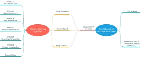
The summit of the Antarctic Ice Sheet, i.e., Dome A, has been a focus area for polar studies. The local air temperature has been an essential element of Antarctic meteorological observations [
1,
21,
22]. However, prior to the arrival of the Chinese Antarctic expedition in 2005, regular air temperature observations were not recorded in the Dome A region. This study developed an approach estimating the instantaneous air temperature from the ice surface temperature by using in situ air temperature observations ever since 2005 and the ice surface temperature retrieved from AVHRR satellite data. Meteorological parameters, including radiations, wind speed, and clouds, were taken into account, and the results from three models (i.e., linear regression, random forest, and neural network) were then compared. If the accuracy is guaranteed, instantaneous air temperature calculations can be carried out in cloudy weather using satellite temperatures. Finally, we simulated the air temperature data in 2004 with a better precision model to make up for the absence of in situ data in 2004.
3. Methods
Thermodynamic relationships exist between the air temperature and skin temperature. The surface energy balance drives the surface temperature and surface melt, so it is important to consider the surface energy balance [
24]. Based on the features of the near-surface layer of the Antarctic Ice Sheet [
1], the surface energy balance can be written as:
where
is the net shortwave radiative flux, Ln is the net longwave radiative flux, and G is the subsurface conductive heat flux proportional to the temperature difference between surface and medium below the surface.
H and
LE are the turbulent sensible and latent heat flux, respectively, and
is the net energy flux at the surface. Note that the turbulent mixing of the lower atmosphere increases as a function of the wind speed.
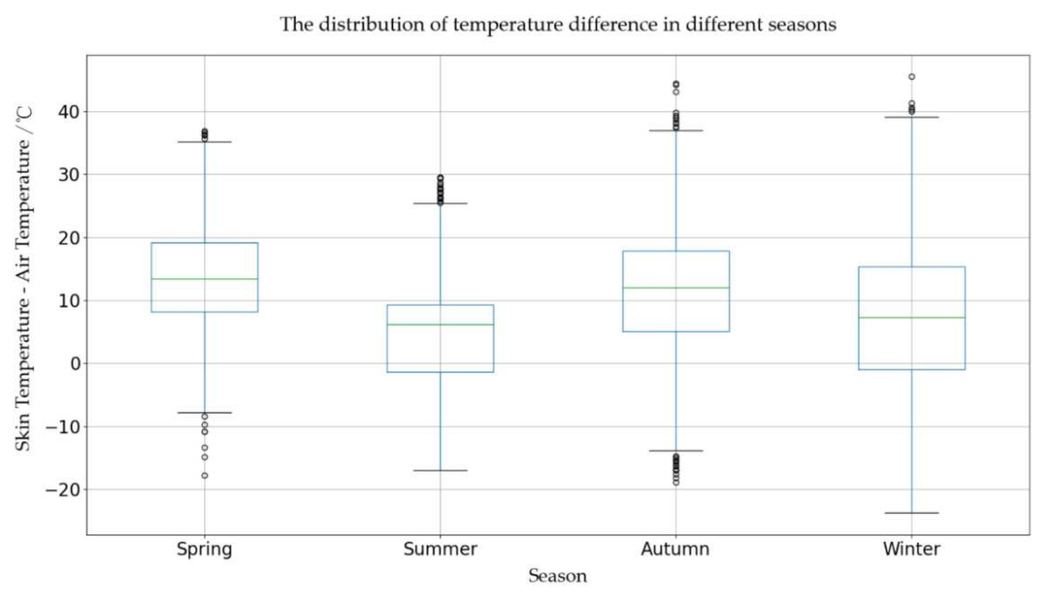
For climate factors, the role of clouds in an energy exchange is complex. On the one hand, clouds reflect and absorb shortwave radiation, which cools the skin. On the other hand, they emit downwelling longwave radiation, which makes the skin warm. In terms of seasonal variability, the skin–air temperature varies over the season, with the smallest differences during the spring, fall, and summer in nonmelting conditions in the Arctic [
18]. Nielsen-Englyst pointed out that the Arctic’s seasonal cycle can be a predictor, assumed to be the shape of a cosine function, to obtain the air temperature [
18]. In this paper, the temporal changes of skin temperature at Dome A were extracted using AVHRR satellite data from 2005 to 2020, as shown in
Figure 3. Note that skin temperatures at the Dome A region also change periodically. The difference between air temperature and skin temperature in 2005–2020 was extracted by season, as shown in
Figure 4. It should be emphasized that the seasons in Antarctica and the Arctic are comparatively different. We follow the definition of a season from Chen (2010) et al. Spring occurs from October to November, summer from December to January, autumn from February to March, and winter from April to September [
22].
From
Figure 4, we can conclude that, in the spring (October to November) and autumn (February to March), the surface temperature at Dome A is usually higher than the air temperature. While the average difference of the temperature between the summer and winter is usually lower than in other seasons, the relationship between the surface temperature and air temperature varies seasonally. In this paper, the longwave and shortwave radiation, wind speed, cloud type, skin temperature, and other seasonal factors were incorporated into the model to predict the air temperatures up to 2 m high.
Among the predictors, the seasonal attribute parameter is a categorical variable, such as the spring and summer. These are not numerical variables that can be put into a model and be directly understood by the computer. One-hot encoding is an encoding technique used in machine learning to process discrete features [
25]. As shown in
Table 3, after using one-hot encoding, we obtained the attribute information for all the categorical variables. For example, the spring is defined as [1, 0, 0, 0], and the summer is defined as [0, 1, 0, 0].
In all modes, 80% of the data (N = 1725) were randomly selected for the training set and 20% for the test set (N = 345) to judge the model accuracy. Ten-fold cross-validation was used to adjust the parameters of random forest and neural network in 80% of the data (1380) to ensure the independence of the training set and validation and test sets. The training set and the test set were the same for all models.The skin temperature, shortwave radiation, longwave radiation, and cloud type were obtained from the pixel nearest to Dome A in the AVHRR-X product. The air temperature at Dome A (in situ data) and wind speed from MERRA-2 perfectly matched the time of the two daily scenes of the AVHRR-X product. It is important to note that the cloud type data is a continuous value; the value in the tens place represents the type of cloud obtained by the CASPR algorithm analysis. For example, “0” means no cloud, and “1” means that the cloud type is cirrus (each number from 1 to 9 has a corresponding cloud type). The values in the ones place are the types of clouds analyzed by the CLAVR algorithm. For example, “0” means “clear or partly cloudy” and “1” means “fog”(each number from 1 to 9 has a corresponding cloud type). Although it is the cloud type that is being read, some information about the cloud fraction can also be inferred from the type of cloud.
3.1. Random Forest Model
Random forest belongs to the family of ensemble machine learning algorithms that predicts a response (in this case, the respective climate parameters) from a set of predictors (matrix of training data) by creating multiple decision trees (DTs) and aggregating their results [
26,
27]. Every tree in a random forest is a Classification And Regression Tree (CART). The branch of CART used in solving regression problems is the mean square error (MSE), and variance reduction is used as the criterion for feature selection. For a dataset containing n samples, the samples are randomly selected each time and then returned to the original dataset so that the samples may still be collected in the next sampling. The process is repeated to obtain different trees that form the random forest. Note that the features are randomly selected from the samples and that the decision tree is built automatically using these features for the selected samples. In addition, not all characteristic variables are used in the construction of each decision tree model, but a subset is randomly extracted from all features to train the model. As for the data to be predicted, each parameter is decided by each tree in the constructed random forest. Each vote has the same weight, and the output is the average of each tree.
3.2. Deep Learning Model
Due to the rapid developments of deep learning, the algorithm has become widely used in numerical prediction, image processing, and other fields [
28,
29,
30,
31,
32]. Commonly used network structures include the convolutional neural network, recurrent neural network, and deep neural network. The convolutional neural network is often applied to images, because when features are extracted from images, the image is regarded as a digital matrix, and the correlation between pixels and local features can be extracted. A recurrent neural network is often used to process time series data and considers the background signal before and after the time period of the current input as being closely related. In general, a deep neural network is often used for prediction; the input contains a series of numeric column vectors, which are the influencing factors of the predicted value. For this study, the main focus was the influence of various factors on the temperature. Due to the use of multi-source data, a lot of data gaps could be found in the continuous time series, which could introduce significant prediction errors into the next period. For long-time series predictions, the recurrent neural network has the tendency of significant error accumulations. Therefore, a deep neural network was used for air temperature prediction in this study.
The neuron receives input signals from n other neurons. These signals are transmitted through weighted connections, and the total input value received by the neuron is compared to the neuron’s threshold. The output of the neuron is produced by activation function processing. The existence of the activation function makes the model have a nonlinear structure to handle more complex things. In this study, ReLu was used as the activation function. When the activation function threshold was reached, the neuron signal was transmitted; otherwise, the neurons were suppressed.
In multi-layer network learning, an error Back Propagation (BP) algorithm is used to train the datasets. The algorithm adjusts the weights and biases on each node through learning and making the target closer to the real value. Using the connection weight as an example, the weight adjustment is as follows:
where
is weight change of connection between two neurons at layer
h and layer
j,
is the mean square error between the output and the real value in the training set.
is the learning rate that controls the step size of each round in the algorithm. When the learning rate is too small, the convergence rate will be very slow, and the local minimum will probably be found rather than the global minimum. When the learning rate is too high, it will cause concussion.
Deep learning models are very deep neural networks. For neural network models, an easy way to improve their understanding is to increase the depth of the network. The larger the network depth, the more the parameters (e.g., neuron connection weight and threshold value) available to complete more complex learning tasks. The complexity of the model can also be increased by increasing the number of neurons in a single layer. However, errors are constantly transmitted between neural layers. When the depth is too large, errors tend to diverge during transmission and fail to converge to a stable state, which could even cause the gradient to disappear.
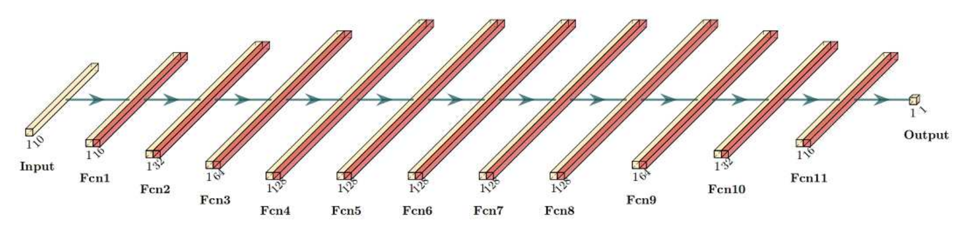
For this study, the neural network model needs to be optimized by artificially adjusting the number of neurons in each layer and the depth and learning rate of the neural network. As shown in
Figure 5, a deep neural network (DNN) uses the numerical data as the input, processes the data layer by the stratum through the hidden layer (11 layers; the number of neurons in each layer is as follows in
Figure 6, for example. The first layer has 16 neurons, and the second layer has 32 neurons.) and, finally, generates the data through the output layer. The process of adjustment for the parameters of neural networks will be mentioned in
Section 4.
4. Results
The parameters of each factor in the linear regression model are shown in
Table 2. Note that the attribute value of the seasonal factor is 1. It means the coefficient of one season at a certain time is 1, while the coefficient of the other three seasons is 0. In linear regression, the coefficients of each factor indicate the importance of that factor to some extent. Based on the regression results in
Table 2, there is a strong linear relationship between the 2-m eastward wind and skin temperatures from the satellite image and air temperature. Additionally, the influence of 2-m eastward wind on the air temperature at Dome A is generally a warming effect.
In the construction of the random forest model, one major problem is parameter adjustment. The parameters that have to be adjusted include the number of trees in the random forest (n_estimators), the maximum depth of the decision tree (max_depth), and the maximum number of features in the selected feature subset (max_features). In order to find the optimal value for the parameter needed to be adjusted, the parameter is constantly being debugged within a reasonable range. When testing for the optimal value of a single variable, the other variables are kept unchanged. After finding the optimal value of one parameter, it is used in the subsequent tests to find the optimal value for the other parameters.
The score indicates the prediction accuracy. In
Figure 6, the score is determined using Equations (3)–(5), where
refers to the value in model regression,
is the actual value of sample i, and
is the average of the real value. The larger the value of the score, the higher the accuracy of the model. Both the test set and the training set were used in evaluating the model. The score of the training set represents the fitting strength of the model, while the score of the test set indicates its generalization ability. As shown in
Figure 6, when the threshold is reached, the model accuracy does not increase even when the n_estimator, max_depth, and max_features are increased. In the model, the values for the n_estimator, max_features, and max_depth were set to 99, 9, and 22 (the optimal parameters of n_Estimators was firstly found; then, the parameters of Max_depth and Max_feature were adjusted).
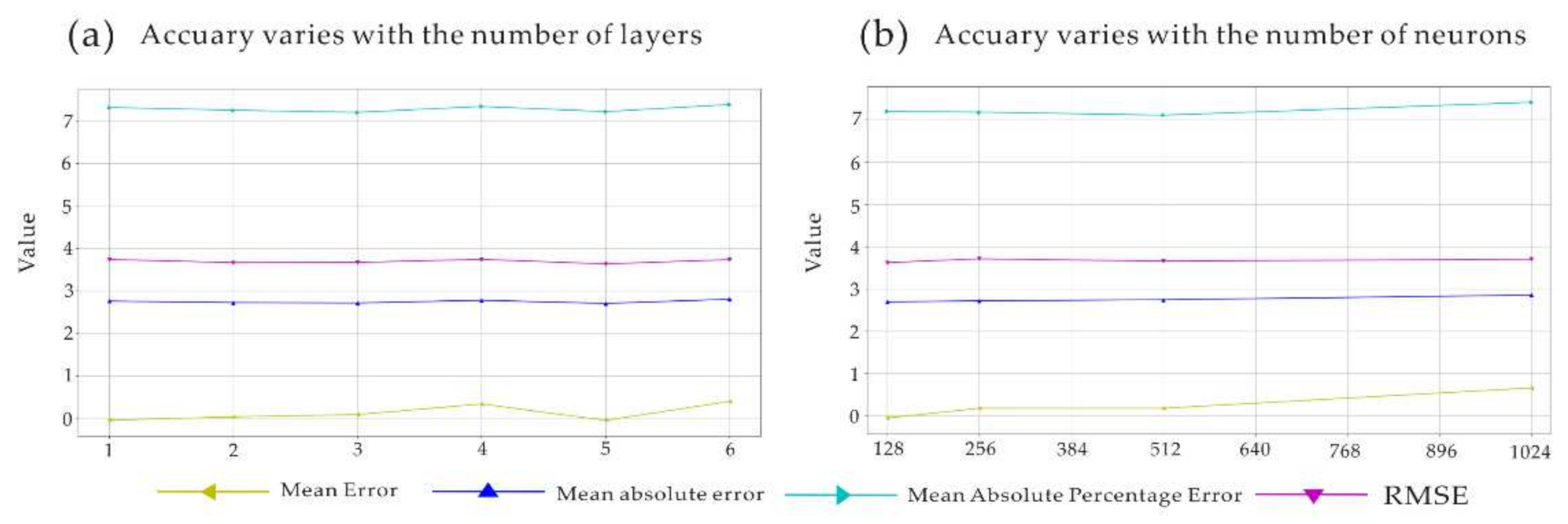
Manual adjustment cannot be avoided in the construction of an artificial neural network. Firstly, the number of layers of the neural network was adjusted. Through a large number of pre-experiments, the network structure of 16-32-64-128-64-32-16-1 was determined to be the great structure, and the model was further optimized on this basis (This network structure can be similarly understood as a decoder and encoder. Before the fourth layer, it functions like an encoder. After the fourth layer, it functions like a decoder. This pyramid structure enable neural networks to learn high-dimensional features.). Starting with the fourth layer, we added more layers of 128 neurons. The results are shown in
Figure 7a, when the number of layers in which the number of neurons is 128 reaches five, and the model is optimal from the mean error, mean absolute error, mean percentage error, and RMSE. After the layers of the neural network were determined, we changed the maximum number of neurons using 16-32-64-128-128-128-128-64-32-16-1 as the benchmark. As shown in
Figure 7b, the model reached the best from the mean error, mean absolute error, mean percentage error, and RMSE when the maximum number of neurons was 128. Finally, the model of the neural network was determined.
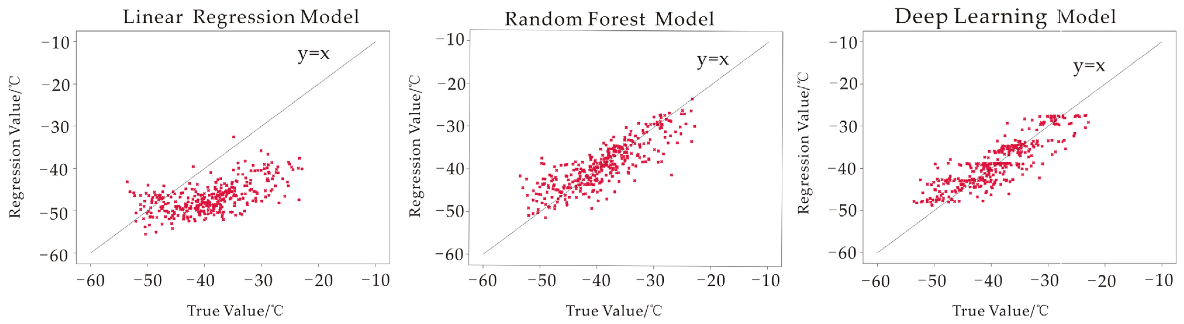
The fitting effects for the three models are shown in
Figure 8. Based on the results, the values predicted by the linear regression model were generally lower than the true values, and the random forest model had the best fit. The models were evaluated using mean bias, MAE, MAPE, and RMSE, and a summary of the results is shown in
Table 4.
For missing temperature measurements, we prefer to simulate the model using the available reanalysis data and satellite data. In the above analysis, we used 15 years of data for training to build a high-accuracy model.
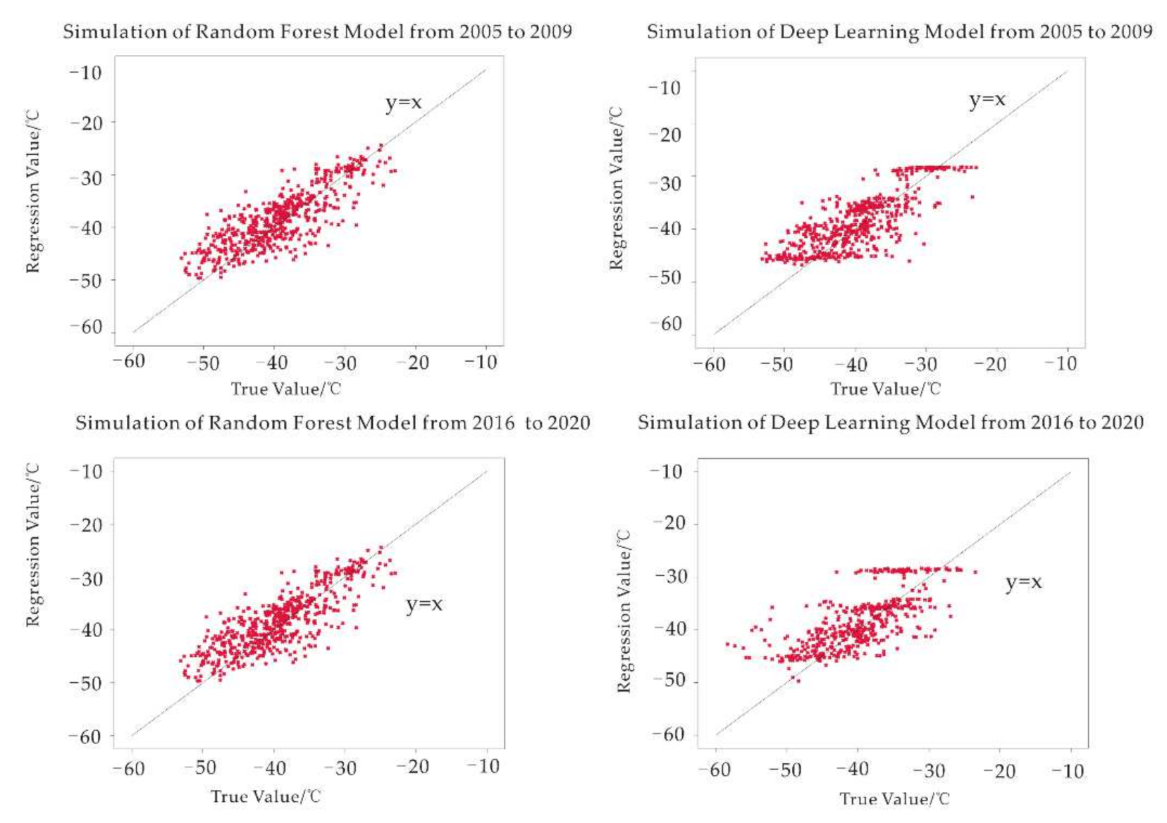
When measured data is missing, can the model be used to simulate the temperature regardless of the time difference? Given the high accuracy produced by the random forest model and deep learning, we used the 2010–2015 data as the training set to find the quantitative relationship between the climate factors and air temperature. The temperature data for 2005–2009 and 2016–2020 were then simulated, and the simulation results are presented in
Figure 9.
From
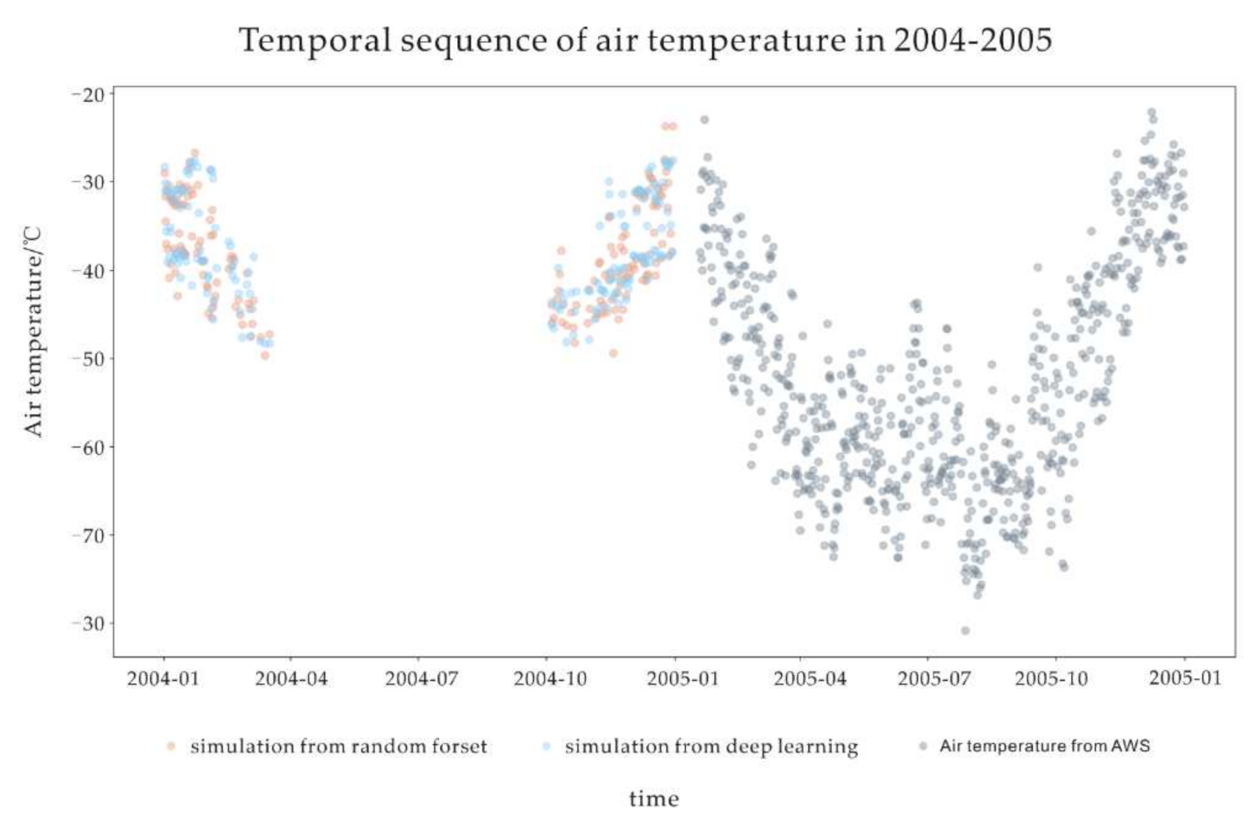
Table 5,The random forest and deep learning approaches yielded high-accuracy simulation results for 2005–2009, with average biases of 0.86 °C and 1 °C and RMSE values of 3.76 °C and 3.94 °C, respectively. The results suggest that it is possible to simulate past missing data. Data from 2005 to 2020 were then put into the two models for training, and the missing data for 2004 were simulated. The results are shown in
Figure 10. Both models estimate that the temperature starts to cool down in January and increases in October. In both the random forest and deep learning methods, the highest temperature appeared in the summer at Antarctica at −23.72 °C (2004/12/30) and −27.54 °C (2004/1/23), respectively. The simulation results can be comparable with the actual maximum air temperature for 2005–2020, as presented in
Table 6.
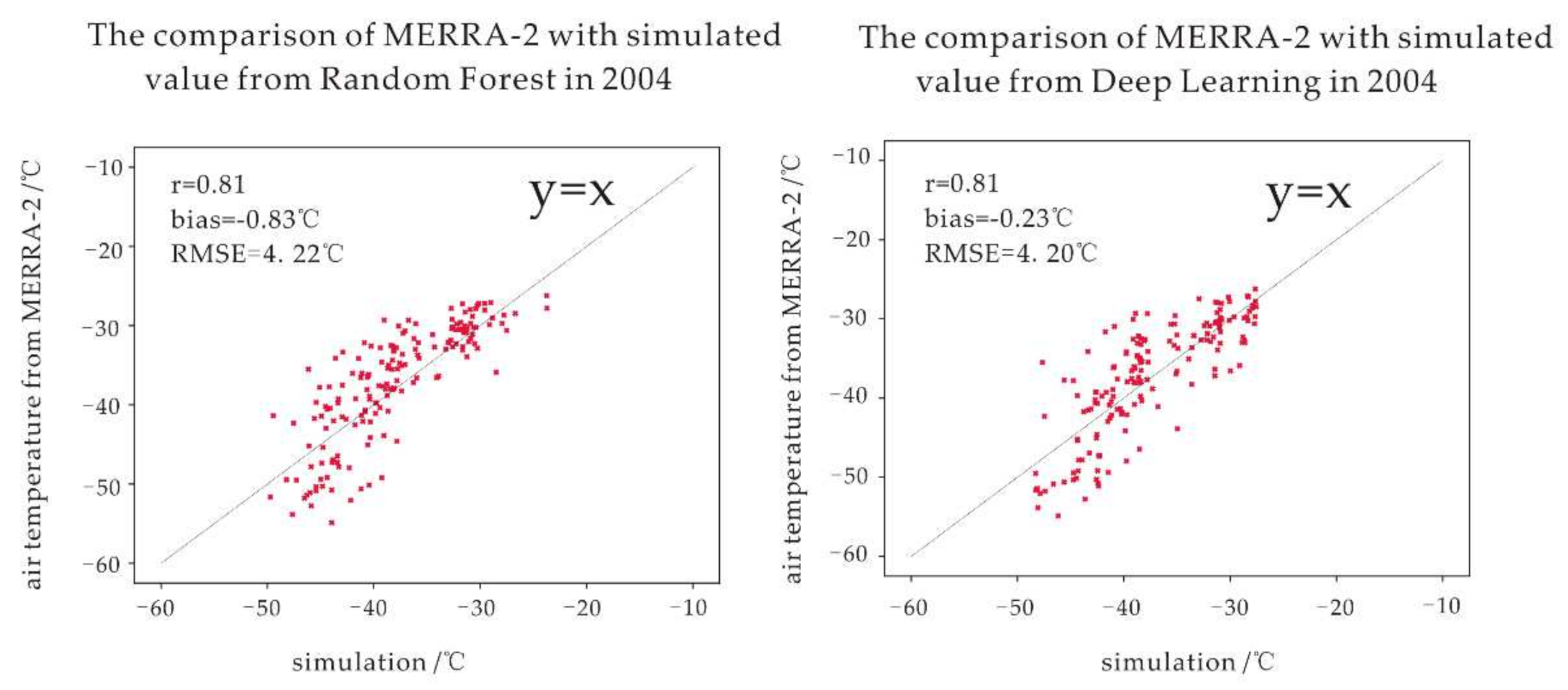
In addition, we compared the simulation at 2004 obtained by random forest and deep learning with MERRA-2. The result is shown as
Figure 11; the simulated values of the two models have good coupling with MERRA-2. The average deviation of the simulated instantaneous temperature is low, which indicates that the monthly average temperature obtained by the aggregation of the simulated values is highly reliable.
For the deep learning results, both the simulated (2005–2009) and the predicted (2016–2020) values tend to be about −30 °C, with a large number of points forming a horizontal line, as shown in
Figure 9. Therefore, the threshold for extracting the predicted and simulated outliers was set to −30 °C (see
Figure 10). As for the thermodynamic factors, the outliers have similar Pearson coefficients for longwave radiation (−0.51 and −0.38) and northward winds (0.3 and 0.18) in
Figure 12.
5. Discussion
The accuracy is a very important criterion to judge the model; previous studies have largely focused on nonpolar regions. Regardless of the method used, the RMSE in many of these previous studies generally fell between 2 and 3 °C [
13]. The polar regions amplify the Earth’s climate and experience extreme weather conditions. Little research has been done in these areas because of their harsh conditions. The error will also increase in relevant experiments, especially in Antarctica. In this paper, the accuracy in the deep learning (RMSE = 3.42 °C) was consistent with the accuracy of the model Nielsen-Englyst et al. [
18] came up with at Arctic, and the instantaneous air temperature could be estimated under complex conditions.
In our study, for the deep learning model, there was a certain amount of simulation value fluctuation at −30 °C in the simulations of 2005–2009 and 2016–2020. In terms of the climatological factors, the simulated values of the first five years had similar Pearson coefficients with those of the second five years for longwave radiation and northward-wind. In general, the simulation accuracy of both models in the first five years was higher than that in the last five years, so it is possible for both models to simulate the missing data in the past.
As can be seen from
Figure 3, the surface temperature achieved the maximum in 2018 to 2019. The simulation air temperatures at 2018 and 2019 both have large biases and variations. The random forest (2018: bias = 2.23 °C, RMSE = 6.34 °C; 2019: bias = 1.47 °C, RMSE = 4.88 °C) and deep learning (2018: bias = 2.60 °C, RMSE = 5.73 °C; 2019: bias = 1.96 °C, RMSE = 5.0 °C) both produced large errors. Noguchi et al. [
33] studied the response of the Antarctic troposphere to a stratospheric warming event in September 2019 and pointed out that polar warming is great influenced by this very strong Brewer-Dobson circulation. It is possible that the events of extreme weather in 2018 to 2019 changed the connection between matter, and the model lacked the learning of extreme events when training data from 2010 to 2015, so the accuracy of the machine learning decreased.
Compared with deep learning and random forest, the test set of linear regression showed a large error. However, linear regression can be used to statistically analyze the effects of different climatic factors on air temperature. For example, we learned that 2-m eastward wind at the Dome A region has a warming effect on air temperature at a height of 2 m from the coefficient of linear regression. For deep learning and random forest, although they both have high accuracy and a certain anti-interference ability, the model was just a black box, and we could not analyze whether climate factors have a positive or negative impact on air temperature.
The use of multi-source data also brings a series of problems. The first is the resolution of different data. The in situ data comes from automated weather stations and represents a point, while the individual pixel values of the reanalyzed data and the AVHRR satellite data represent the values of an area. Are the in situ temperatures at the weather station representative of the air temperatures over the area? Hall et al. [
34] found that the surface temperature of in situ data changes measured in the field were within 1 °C on a 1-km scale over the Greenland Ice sheet in the Arctic, and the temperature variation was mainly determined by surface roughness. Snyder et al. [
35] pointed out that, in uniform and flat surfaces that can be easily measured and characterized, including inland, water, sand, snow, and ice, the measured temperature at the site can be used as a verification of the temperature products at the pixel scale. That is, once the region is determined to be uniformly heated, the measured data can represent the temperature of a certain region. Dome A sits on the Antarctic Plateau, with thin air and low wind speeds, and has an extremely flat, smooth surface. It is theoretically appropriate to treat the measured temperature as a regional value. Secondly, the simulation of temperature depends on specific environmental factors; that is to say, for the simulation of instantaneous temperature, when a certain kind of data is missing in this time series, the model will not be used. Therefore, simulations for air temperature in a time series from April to September is still lacking.
6. Conclusions
In this study, we proposed three methods: linear regression, random forest, and deep learning to estimate air temperature from satellite surface temperature. All models incorporated seasonal factors, cloud type, wind speed, short-wave radiation, long-wave radiation, and surface temperature as predictors of energy transfer over the surface of the Antarctic Plateau. In terms of the accuracy of the model, the deep learning effect was the best. The MAE of the test sets was 2.65 °C, and the RMSE was 3.42 °C. Random forest followed with a MAE of 2.77 °C and RMSE of 3.70 °C. The ability of the model to simulate missing data in the past was also evaluated. The data from 2010 to 2015 were trained by a deep learning and random forest model; then, the air temperature data from 2005 to 2009 and 2016 to 2020 were estimated. In the random forest, the mean deviation of temperature from 2005 to 2009 was 0.86 °C, and the RMSE was 3.76 °C. The average deviation from 2016 to 2020 was 1.04 °C, and the RMSE was 4.61 °C. In the deep learning model, the average deviation of the temperature from 2005 to 2009 was 1 °C, and the RMSE was 3.94 °C. The mean deviation of the temperature from 2016 to 2020 was 1.26 °C, and the RMSE was 4.56 °C. According to the simulation results, the generalization ability of random forest was similar to that of deep learning in this modeling.
Finally, the data from 2005 to 2020 were trained in a random forest and deep learning model to simulate the missing temperature data in 2004. In comparison with the simulated values of 2004 and MERRA-2, it was found that the mean deviation of the instantaneous temperature simulated by deep learning was low (−0.23 °C). This means that the monthly mean air temperature aggregated from the simulated values had a high degree of confidence. This paper provided a method to generate a supplement for the monitoring of 2-m air temperatures at Dome A in a time series.


 ,
, 


