Article

The River–Sea Interaction off the Amazon Estuary

1
Key Laboratory of Submarine Sciences and Prospecting Techniques, MOE, Ocean University of China, Qingdao 266100, China
2
College of Environmental Science and Engineering, Ocean University of China, Qingdao 266100, China
3
College of Information Science and Engineering, Ocean University of China, Qingdao 266100, China
4
Qingdao Blue Earth Big Data Technology Co., Ltd., Qingdao 266400, China
*
Author to whom correspondence should be addressed.
Remote Sens. 2022, 14(4), 1022; https://doi.org/10.3390/rs14041022
Submission received: 29 December 2021 / Revised: 14 February 2022 / Accepted: 16 February 2022 / Published: 20 February 2022
(This article belongs to the Section Ocean Remote Sensing)

Abstract

:
The Amazon River has the highest discharge in the world. Nevertheless, there is still a lack of the research on the interaction between river-diluted water and the ocean. This study used the remote sensing data (2008–2017) of the Moderate Resolution Imaging Spectroradiometer (MODIS) aboard the Aqua satellite, and data of the currents, wind fields, sea surface temperature, and water depth. The river–sea interaction off the Amazon estuary was studied by analyzing the diffusion of river-diluted water and the distribution of surface suspended particulate matter (SPM). The results revealed that the Amazon estuary has a “filter effect,” whereby the distribution of the surface SPM exhibited significant spatial characteristics of being high in the nearshore area and low in the offshore area. Most of the SPM accumulated within the estuary in a fan shape, although some was distributed in the shallow water region of the continental shelf along the coasts on both sides of the estuary. The currents were found to limit the diffusion range of SPM. The flow direction and velocity of the North Brazil Current and the North Equatorial Countercurrent, which are largely driven by the magnitude of the trade wind stress, are the main forces controlling the long-distance diffusion of diluted water, thus forming unique river–sea interaction patterns in the Amazon estuary. This research provides a supplement and reference for the study of the diffusion process of SPM and river-diluted water, and on the estuarine river–sea interactions of other large rivers worldwide.

1. Introduction

Surface suspended particulate matter (SPM) has a significant impact on the water environment, and is one of the three factors affecting the color of the ocean. In addition to comprehensively reflecting natural environmental conditions, the concentration distribution of the SPM is also an important manifestation of the river–sea interaction in estuarine areas [1]. The Amazon Basin is located in the northern part of South America (Figure 1) and originates in the Andes Mountains in the western part of South America. The Amazon Basin drains a catchment area of 5.9 × 10⁶ km2 and has more than 1.5 × 10⁴ tributaries, a mean annual discharge of 2.08 × 10⁵ m3/s [2], a runoff length of 6400 km, and an annual sediment discharge of more than 8.0 × 10⁸ t [3]. The annual mean discharge rate onto the north Brazilian shelf at the equator is (1.93 ± 0.13) × 105 m3 s−1 [4], and 82% of the suspended sediment transported by the Amazon was contributed to by 12% of the total drainage area, including the Andes Mountains. Most of the sediment discharged by the Amazon River originates from the rapid erosion process in the Andes Mountains, which accounts for about 12% of Amazonian land [5] (p. 46). The Amazon River’s lower course is very flat: 20 m of variation in level over the last 1500 km, so the river flow is dependent largely on the upper water discharge and tides. It needs to be emphasized that the flow is so strong that seawater never enters the estuary, resulting in a large pool of brackish water beyond the mouth [6]. Thus, the Amazon Basin has the largest discharge, basin area, and number of tributaries of rivers basins worldwide.
Research on the river–sea interaction and sediment transport of the Amazon River began with Gibbs [7,8], who studied the types of sediment at the bottom of the Amazon River along with the concentration and distribution of SPM. According to measured data, Gibbs [9] proposed a model in which water moving from the Amazon estuary to the sea diffused as surface plume, mixed with seawater in the upper layer, and then flowed northwestward along the outer continental shelf under the influence of currents. Richey et al. [10] showed that the maximum and minimum flows of the Amazon River occurred in May–June and October–November, respectively, and the maximum of surface SPM occurred between February and March. The SPM entering the continental shelf was bound in the mixed flow of fresh water and seawater, and then extended hundreds of kilometers along the coasts towards the sea and northwest region. The SPM varied from a few milligrams per liter to one gram per liter, and did not flow with low-salinity surface plumes. An estimated 85–95% of the sediment discharged by the Amazon River is suspended silt and clay-sized particles [11].
Lentz [12] considered that the diluted water of the Amazon estuary could spread 100–200 km from the estuary towards the frontier area of the inner continental shelf. The SPM in the shallow shoals of the Amazon estuary, and in the high turbidity area between the estuary and the sea near the northwest coast, is higher than that of the Amazon River, which may be due to resuspension and strong mixing [13]. Kineke et al. [14] also studied the transport of fluid mud (a type of high-concentration suspended sediment) over the Amazon continental shelf. Approximately 5% of the suspended sediment was transported by low-salinity plumes, whereas 7–17% was transported via the northwestward (near the coast) advection transport of the shelf system and 35–70% settled on the shelf. Park et al. [15] used Moderate Resolution Imaging Spectroradiometer (MODIS) data to simulate the distribution of surface sediments off the Amazon River by estimating the concentration of surface sediments. Vantrepotte et al. [16] emphasized the relationship between the migration of mudflats and the interannual variation of the SPM assessed by satellites in coastal waters and proved that the variation in the SPM of the Amazon estuary is associated with seasonal variations of the trade winds. Based on satellite data, Gensac et al. [2] evaluated the input of fine-grained sediments from the Amazon River into the sea as well as their transport via river–sea interactions and found that fine-grained sediments were transported northward to the Orinoco River delta along the coasts. Chérubin and Richardson [17] expounded that the freshwater plume extends northwestward across the eastern Caribbean Sea, starting in July–August and continuing until October–November on the Amazon Shelf. Others also researched the dispersal of the Amazon and Orinoco River water in the tropical Atlantic and Caribbean Sea based on SeaWiFS [4,17,18].
Previous studies on SPM were mostly based on measured oceanographic research data, which are both temporally and spatially limited. Remote sensing methods have been used to analyze the river–sea interaction in the Amazon estuary and the dynamic process of driving its diffusion. However, these studies lacked systematically seasonal comparative analysis. Remote sensing satellites can quickly and effectively monitor the distribution of and change in surface suspended sediment with a short data acquisition period and good synchronization. In previous studies, MODIS data were processed by a single band analysis method [2], the time scale was short [4], or model results were used to explore the sediment distribution pattern in the Amazon estuary area [19]. MODIS data have the obvious advantages of high resolution and continuous temporal coverage. In this work, a relatively new long-term time series (2008–2017) was selected, and we adopted a data-processing method more suitable for nearshore turbid water, supplemented by measured data for verification. MODIS data were utilized to analyze the spatial and temporal variations of SPM and river-diluted water off the Amazon estuary. The basic characteristics and patterns of the river–sea interaction in the Amazon estuary are revealed. This research supplements the study of the diffusion process of SPM and river-diluted water and could provide a reference for the study of estuarine river–sea interactions of other global large rivers.

2. Materials and Methods

2.1. Data Sources

In this work, L1b data (2008–2017) of the MODIS aboard the Aqua satellite (National Aeronautics and Space Administration (NASA, Washington, DC, USA), https://www.nasa.gov (accessed on 13 October 2020)) were collected. The data have a wide coverage and strong temporal continuity, with a spatial resolution of 1 km. MODIS images were constantly available for consecutive months for long-term monitoring of tropical areas by remote sensing means, and they provide unprecedented knowledge for much larger areas than a monitoring network would allow [20]. Compared with traditional measurements, satellite data provide a more effective and convenient way to analyze the diffusion path and transport patterns of marine SPM. For example, the SeaWiFS bands of 555, 670, 765, and 865 nm have the greatest spectral response to SPM, whereas the SeaWiFS bands of 412, 443, 490, and 510 nm have a high response to Chromophoric dissolved organic matter (CDOM), chlorophyll pigments, and atmospheric aerosol variability. The 555 nm band is highly sensitive to low SPM concentration and is not impacted by light absorption from phytoplankton pigments [21], as is the 443 nm band to CDOM.
CDOM, known as “yellow matter,” is dissolved organic matter containing rich acids, humic acids, aromatic polymers, and other substances. Together with suspended sediment and plankton, CDOM constitutes one of the three major factors affecting ocean color, resulting in yellow or brown water after absorbing ultraviolet and visible light. Previous research results and measured data have shown that the concentration of CDOM in coastal areas is usually negatively correlated with sea surface salinity (SSS) [22,23,24,25]. Plenty of studies took CDOM as a proxy or converted it to SSS, and linear correlations between CDOM and salinity in river plume waters are well documented in the ocean color literature, with reported relationships robust enough to allow salinity retrievals from CDOM [19,26,27]. Therefore, the 555 nm and 443 nm bands were selected in this work to analyze the SPM and CDOM in the Amazon estuary, respectively. The absorption coefficient of CDOM (aCDOM) was selected to calculate the salinity of the seawater, thereby indicating the diffusion path of diluted water off the Amazon estuary.
The wind field data were derived from the meridional and zonal wind data set Cross-Calibrated Multi-Platform (CCMP, Santa Rosa, CA, USA, http://www.remss.com/measurements/ccmp/ (accessed on 19 April 2019)) and were provided by the Physical Oceanography Distributed Active Archive Center at NASA. The data have a spatial resolution of 0.25° × 0.25° and a temporal resolution of 6 h. This wind field is superior to the Q/N hybrid wind field, ERA-40 sea-surface 10 m wind field, and National Center for Environmental Prediction (NCEP, Silver Spring, MD, USA) wind field in terms of spatial resolution and data accuracy; thus, it is recognized internationally at present [28].
The ocean current data were derived from the Simple Ocean Data Assimilation reanalysis data (SODA, Boulder, CO, USA, https://www.atmos.umd.edu/~ocean/ (accessed on 19 April 2019)) and were developed by the University of Maryland (College Park, MD, USA, spatial resolution of 0.25° × 0.25°, vertically divided into 40 layers). They are widely used in the research on global and regional ocean dynamics [29,30,31].
The water depth data were derived from the global topographic surface elevation data (Eptopo1, https://www.ngdc.noaa.gov/mgg/global/global.html (accessed on 1 February 2021)), which were provided by the National Oceanic and Atmospheric Administration (NOAA), with a spatial resolution of 1′ × 1′.

2.2. Methods

In this work, we used NASA’s SeaWiFS Data Analysis System (SeaDAS) software to batch process the data into L2 remote-sensing reflectance (Rrs) data based on the remote sensing data of the MODIS aboard the Aqua satellite. A multiband quasi-analytical algorithm (QAA_v6) [32], which was upgraded from the original algorithm QAA proposed by Lee et al. [33], was demonstrated to be more suitable for the retrieval of absorption coefficients at 555 nm for the inversion of the inherent optical properties of waterbodies, and was used to obtain the particle backscattering coefficient (bbp) and absorption coefficient (a). The above coefficients were utilized to characterize the SPM and aCDOM. Numerous previous studies used the algorithm QAA to study the surface waters of open ocean and coastal areas, such as the Arctic Ocean [34], the Yellow Sea [35], the Yangtze Estuary [36], Tampa Bay in Florida [37], and so on. The reference wavelengths of 443 nm and 555 nm were selected to meet the calculation conditions of the QAA. The NIR-SWIR algorithm proposed by Wang and Shi [38], which is suitable for nearshore turbid waters, was used for atmospheric correction.
Although an empirical negative correlation between the absorption coefficient of CDOM (aCDOM) and the salinity of seawater was usually used in previous works, there were still many variabilities both in the temporal and spatial scales. For example, the relationship was significant only in the nearshore stations [23]. The negative correlation between sea surface salinity (SSS) and aCDOM is time-dependent to a certain extent; aCDOM varies greatly in different river flow seasons and months [39]. We may lack relevant synoptic analysis, or even a mismatch between the water observed by the satellite and shallowest float observation [4]. The selected algorithm may also have a certain effect on the applicability of specific research areas. Therefore, in order to make the study more convincing, correlation analysis was conducted for aCDOM and the measured salinity data provided by Qingdao Blue Earth Big Data Technology Co., Ltd. The inversion formula of SSS and aCDOM was also established to characterize the seasonal variation of diluted water and SPM based on 7606 measured salinity values. We matched the measured data points with remote sensing points within 2 km on satellite images and finally found 1063 matching points. We used robustfit to obtain a robust regression coefficient by eliminating outliers so that the fitting method was less affected by outliers. It eventually showed that there was a good nonlinear negative correlation between salinity and CDOM (especially in low-salinity areas near the Amazon estuary, Figure 2). The inversion formula is:
SSS = 157.9 × ( a CDOM ) 0.04686 152.7
The aCDOM was calculated by QAA_v6 algorithm [32]. SPM and the calculated SSS could be satisfactory indicators of the transport path and the seasonal variation of diluted water.
Note that the presence of clouds in this region was significant, especially in the tropical areas. Sometimes the cloud cover could even reach 99.96% in the study area. Thus, we selected the bands with the least cloud influence, and weakened its influence by atmospheric correction and a cloud removal algorithm. The data of ocean current, wind field, SPM, salinity, and water depth were adopted to analyze the diffusion path and seasonal variation of SPM and river-diluted water off the Amazon estuary. The coupled patterns of the river–sea interaction in this region were condensed based on the mean state of the above elements.

3. Results

Located near the equator, spring, summer, autumn, and winter are during September–November, December–February, March–May, and June–August in the study area, respectively [40]. To better analyze the process and mechanism of the river–sea interaction in the study area, after accounting for the variation rules of various indicators, June–November and December–May were defined as the “winter period” and the “summer period” in the southern hemisphere, respectively. The influences of various factors on the diffusion of SPM and river-diluted water in the Amazon estuary were analyzed.

3.1. Spatial Distribution and Diffusion of Surface SPM

In order to clearly show the detailed features of different months averaged by multiple years, the deviation between the monthly average and annual average of Rrs was calculated, as shown in Figure 3. The most significant feature lay in the spatial difference of the SPM distribution in the coastal region. Most of the SPM was restricted in the coastal area. From August to January (Figure 3c–h, mainly during the winter period), the SPM along the coast off Amazon estuary increased, mostly on the landward side of the 50 m isobath, which gradually varied from zero to a positive value. From February to July (Figure 3a,b,i–l, mainly during the summer period), the SPM along the coast off Amazon estuary decreased, which varied from a positive value to a negative value. The SPM both south of the Amazon estuary and in the northern region showed similar seasonal variability. The SPM gradually increased in the northern region off the Amazon estuary after July, and the northward transport was significant under the action of the coastal current. In addition, wind-induced resuspension also affected the distribution of SPM, including the coastal area in the south of the estuary.

3.2. Sea Surface Salinity Changes off the Amazon Estuary

In addition to describing the diffusion path of the SPM in the study area directly through the SPM features displayed by remote sensing reflectance, another element that can indicate the diffusion path of river-diluted water is the variations in SSS. In this study, SSS was the calculated sea surface salinity obtained by aCDOM from Formula (1).
Figure 4 indicates the diffusion path of river-diluted waters. The total amount of diluted water in the Amazon estuary during the winter period (Figure 4a–f) was significantly larger than that during the summer period (Figure 4g–l). In addition, the area of low-salinity water was the largest during the period from July to September (Figure 4b–d), which may have been the result of the increased river discharge in winter [41]. During the winter period, part of the river-diluted water remained on the continental shelf, and the diffusion range was limited to the 200 m isobath. A small amount of river-diluted water crossed the 2000 m isobath, diffused northwest from 4° N to 10° N, and then gradually mixed with seawater. The diffusion direction of river-diluted water shifted from the northwest eastward and seaward obviously at 6–9° N after June, and the diffusion distance increased, reaching the region east of 37° W. Meanwhile, the diffusion trend of diluted water to the southeast in the study area gradually moved towards 0–2° N, which also reflected the time when the action of currents began to increase (especially in August, Figure 4c). During the summer period, the seaward diffusion range of river-diluted water decreased, and the maximum diffusion distance to the northwest reached 10° N. The total amount of water diluted to the east was relatively small, and the trend was not obvious. Previous studies revealed that the Amazon diluted water could disperse toward the northwest over a broad geographic area to the Caribbean Sea during the first half of year, but it flowed eastward, carried by the currents during the second half of the year [4,42]. Comparing Figure 3 and Figure 4, it can be seen that SSS and SPM off the Amazon estuary presented the same overall trends in the coastal area. The difference was that most of the SPM was captured by the continental shelf and remained within the estuary area, whereas the distance and range of diluted-water diffusion towards the sea became farther and wider, respectively. The diffusion and transport of diluted water and SPM were not synchronized.

4. Discussion

4.1. Potential Factors Affecting the Diffusion of Surface SPM
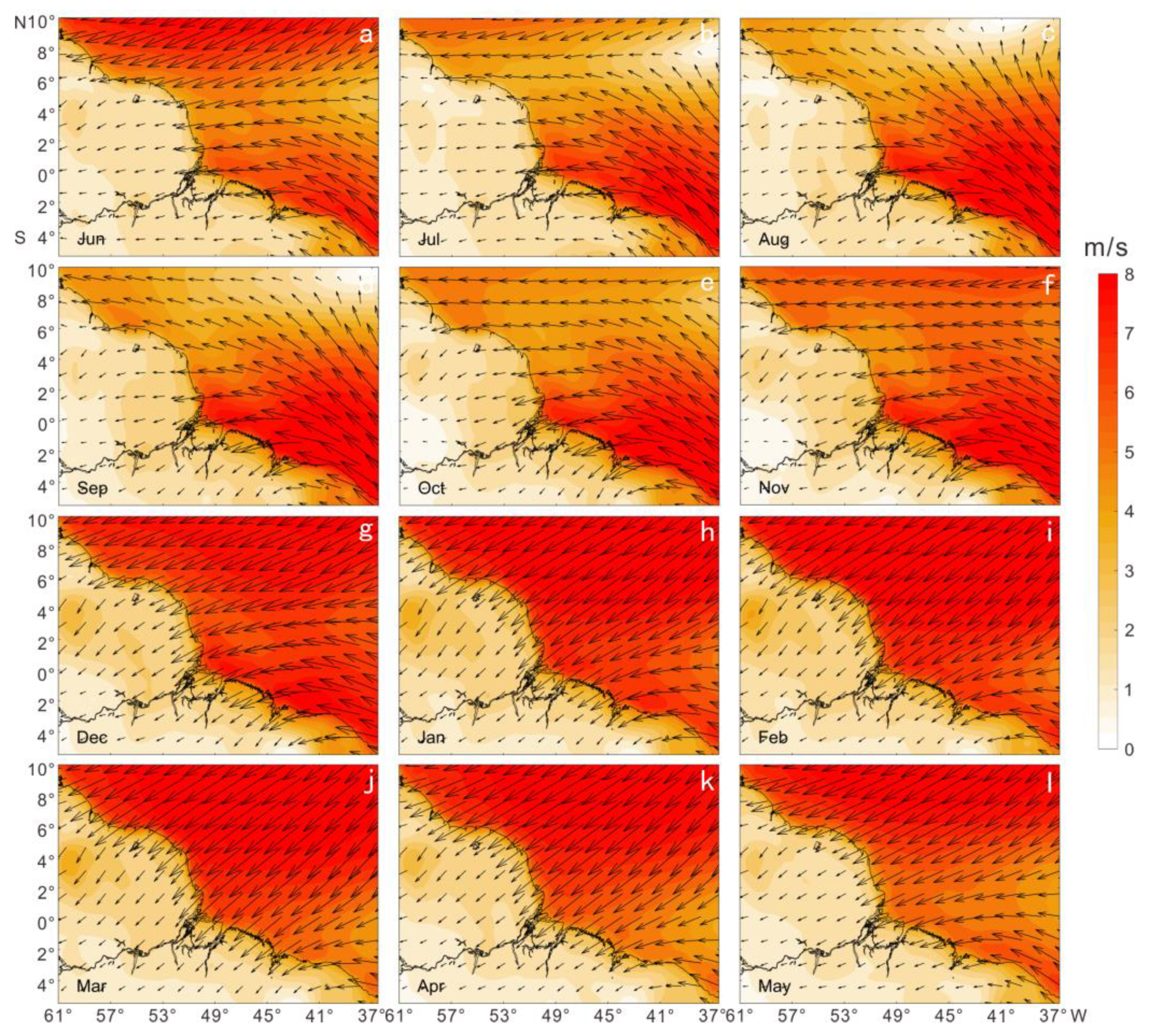
4.1.1. Wind Field

The structure of the wind field in this region was mainly dominated by the trade winds, which greatly influence the currents (Figure 5). The maximum wind speed in the study area generally corresponded to the northeast trade winds during the summer period, whereas the southeast trade winds were the main factor during the winter period. The averaged wind speed gradually increased from 3.5–4.5 m/s to 7–8 m/s from the estuary region towards the sea, with the wind stress significantly increasing during the winter period. In the summer period, the wind speed in the estuary remained at 8 m/s. Lentz’s study [12] showed that although the direction of the northeast trade winds in the summer half of the year was nearly perpendicular to the coast, the components of wind stress along and across the continental shelf had a strong impact on the flow of the Amazon River on the continental shelf, and the river-diluted water continued to carry surface SPM along the coasts. In addition, the trade winds generated surface gravity waves that propagated towards the Amazon continental shelf, causing the largest waves in the estuarine area, where most of the SPM was observed to remain [12].

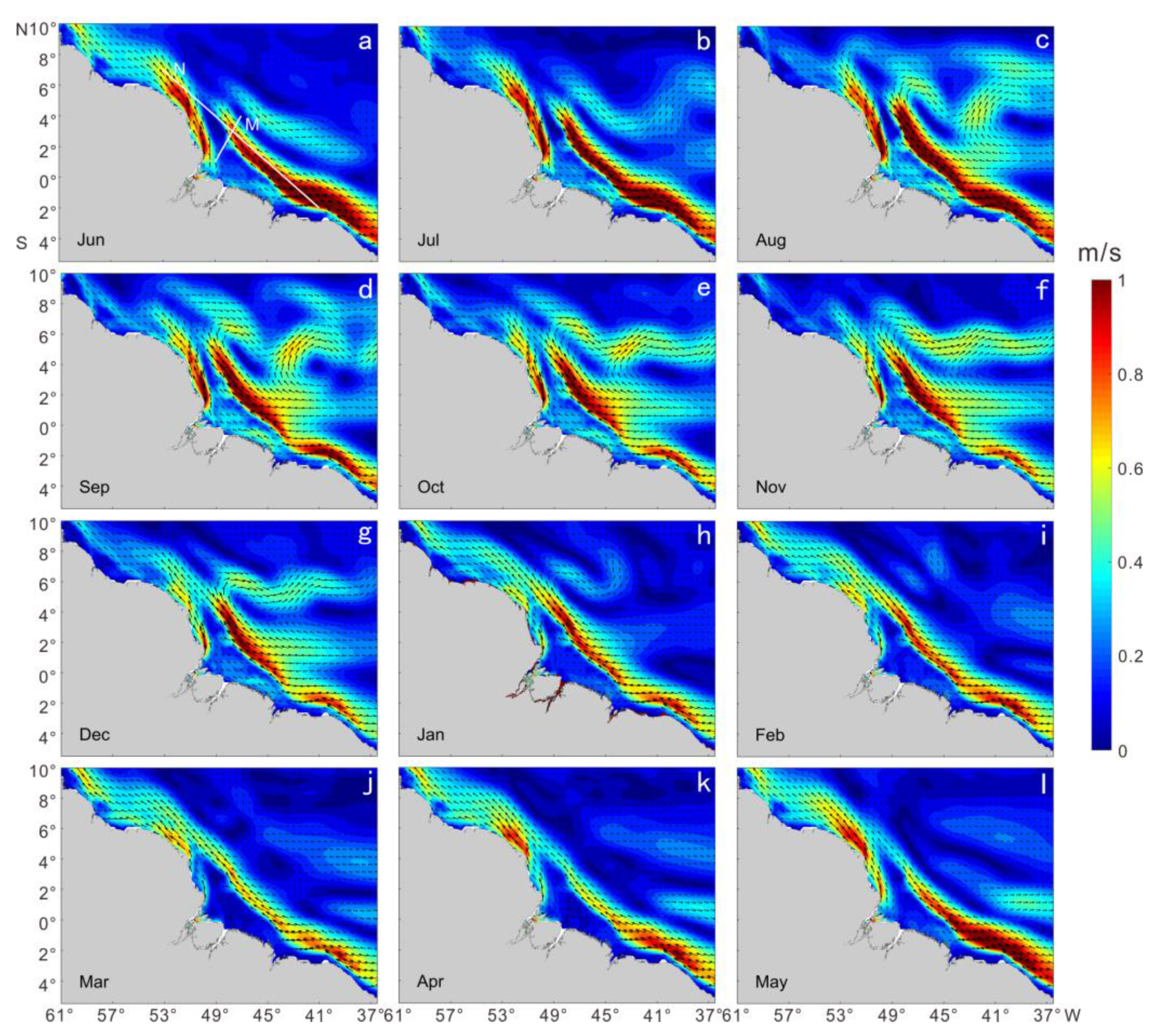
4.1.2. Ocean Currents

There were three main currents off the Amazon estuary: the North Equatorial Countercurrent (NECC), the North South Equatorial Current (NSEC), and the North Brazil Current (NBC). In addition, the Western Boundary Undercurrent (WBUC), the North Brazil Undercurrent (NBUC), the North Equatorial Undercurrent (NEUC), the Equatorial Undercurrent (EUC), and other undercurrents had cycle and supply relationships with main currents. However, the research objective of this study was mainly focused on surface water. Undercurrents with a large depth were not included in our research scope. The recirculation of the NBC supplies the EUC near the equator, and the characteristics of the two vortices were located near 50° W and 44° W (Figure 1) [43]. The reverse curvature of the NBC may have been related to the formation of circulation. These mesoscale vortices moved northwestward along the coast of Guyana, transporting water from the South Atlantic Ocean to the Northern Hemisphere.
The NECC was located between 3° and 10° N and appeared briefly but regularly because the tropical Atlantic circulation was greatly influenced by seasonal winds and had a strong seasonal signal. A study by Grodsky and Carton [44] showed that the NECC began to form in an eastward direction at approximately 6° N in the middle of the Atlantic Ocean due to the northward shift of the trade winds starting in June, which increased significantly during the winter. The NBC was a powerful western boundary current that transported a large amount of water, including the diluted water of the Amazon River. Crossing the equator, the NBC flowed northwestward after passing through the Amazon estuary along the continental edge. Depending on the change in season, the NBC supplied the NECC retrograde, which was most intense in winter [45]. Johns et al. [46] reported that the NBC exhibited large mesoscale transport fluctuations. High-frequency fluctuations were more active in July and August, and low-frequency fluctuations occurred throughout the year, which is consistent with the results of the present study. Compared to the summer period, the currents in the study area developed significantly during the winter period.
Combined with the analysis of Figure 3 and Figure 4, the current speed and direction are the most important factors affecting the river–sea interaction off the Amazon estuary. The diffusion of SPM and river-diluted water in the study area were significantly affected by currents during the winter period. After diluted water discharged from the estuary, it first entrained SPM and diffused northwestward with the NBC, reaching 6° N, where most of the SPM was retained on the continental shelf. The diluted water continued to spread northwestward under the control of the NBC, gradually deviating from the coast and then spreading eastward with the NECC at ~9° N. This caused low-salinity diluted water to spread towards the open sea until it completely merged with seawater. During the summer period, due to the weak development of the NECC and NSEC, the transport of river-diluted water was mainly controlled by the coastal NBC. Therefore, the seaward diffusion trends of diluted water and SPM off the Amazon estuary gradually weakened and almost disappeared.
As shown in Figure 6, the velocity of the NBC decreased sharply off the Amazon estuary and then crossed the estuary to the northwest. The velocity of the NBC increased again at 4° N, leading to an obvious current shear front between the NBC and the sedimentary area off the Amazon estuary. The flow velocity on both sides of the front was quite different: The velocity on the east side was close to 1 m/s, whereas it was only 0.2 m/s on the west side, which was a weak flow region. The large volume of diluted water and high SPM in the frontal zone would have increased the stability of the flow and reduced the effectiveness of tide-induced mixing. As for the tidal currents, although they are very strong on the Amazon shelf, the most important effects are maintaining fluid muds as suspensions [11]. In this paper, the characteristics of the Amazon estuary are discussed from the perspective of river–sea interaction in a long-term scale of 10 years. This average analysis weakens the short-term impact of tidal current on the estuary. The velocity difference between the two sides of the front may also have been due to other factors such as topography.
Comparing Figure 6 with Figure 5, the velocity of the NBC flowing along the coasts gradually increased from 0.6–0.8 m/s to >1 m/s, and the current velocity in sea areas with a high wind speed also increased accordingly. Thus, the trade winds largely drive the direction and velocity of the currents, then cause the diluted water of the Amazon River to spread along the coast or towards the sea under their influence.

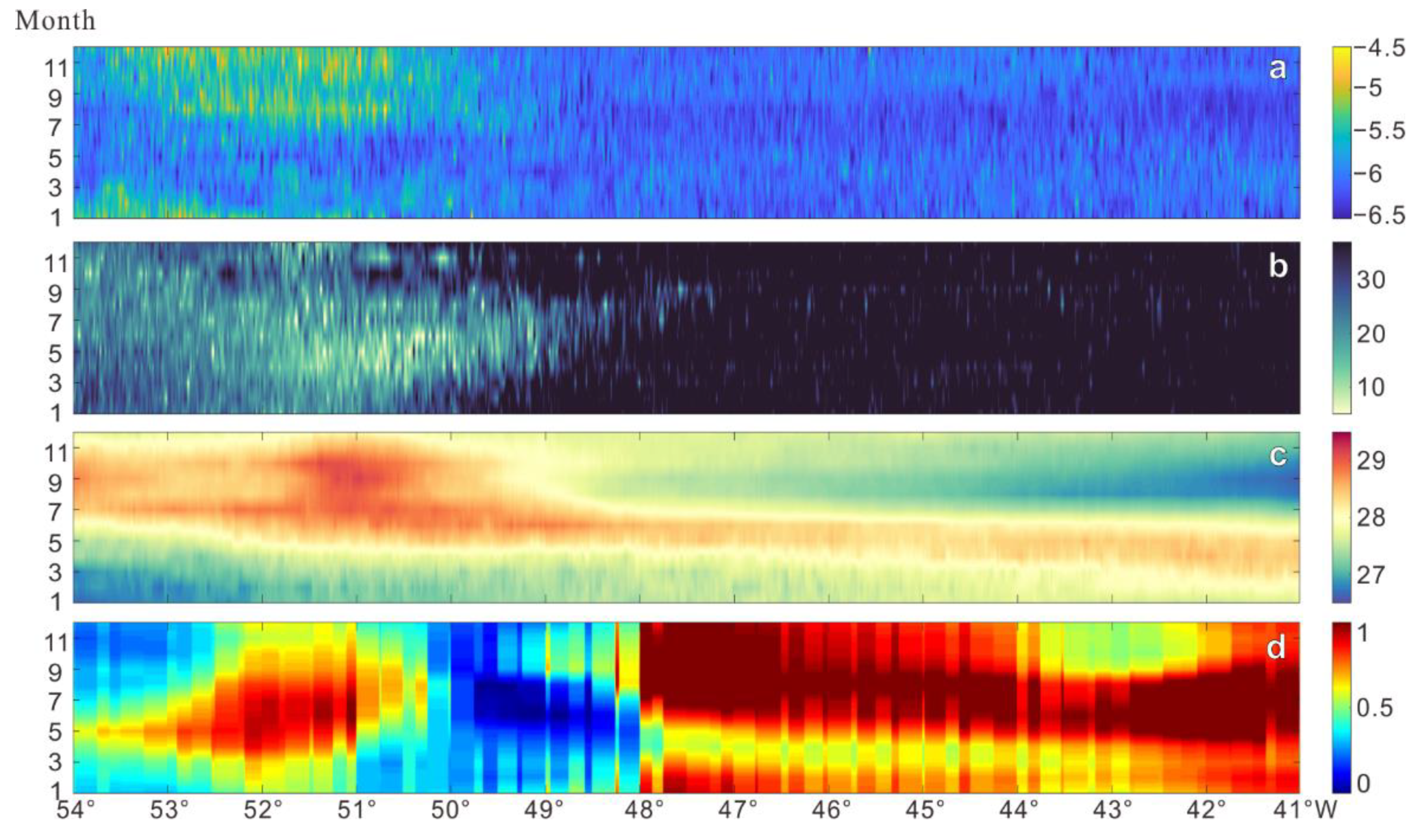
4.2. Transect Analysis

Two typical transects, M and N (shown in Figure 1) that were perpendicular to the Amazon estuary and parallel to the shoreline (along the 200 m isobath), respectively, were selected to further analyze the relationships between the dispersion of SPM and river-diluted water off the Amazon estuary and various driving factors (Figure 7 and Figure 8).
Figure 7a shows the “filter effect” of the Amazon estuary; most of the SPM carried by river-diluted water remained on the shelf (from 49° W to 48.1° W), whereas only a small amount was transported seawards. The research of Curtin and Legeckis [47] concluded that an SPM of >0.01 g/L in surface water extended approximately 200 km seaward. Approximately 60–70% of the sediment discharged by the Amazon River could be accounted for by accumulation rates on the shelf, or by the observed transport towards the northwest due to the strengthening of the coastal current in the northern area of the Amazon River [48,49]. Figure 7b reveals that an obvious seasonal variation appeared in the diffusion of the diluted water, which was significantly enhanced during the winter period. Figure 7c shows that high SSTs were mainly concentrated in the estuary region, and that the SSTs during the winter period were significantly greater than those during the summer period in the southern hemisphere. As the study area is located in the tropical region, its dominant climatic characteristics include rainy, humid, and continuous high-temperature conditions. Therefore, even though there was an interannual variation of SSTs, the maximum SST difference was only 4 °C and the maximum of SST value was approximately 29.5 °C, based on the mean state. Silva et al. [44] proposed that the maximum SST value was affected by a freshwater plume related to the flow of the Amazon River. Overall, the currents developed more in the winter period in the southern region (Figure 7d, there was almost no current flow at the estuary). A shear front existed between the NBC and the coastal waters, where the flow velocity on both sides showed extreme differences at 48.1° W.
Figure 8 shows the changes in various elements over time on a long-distance parallel transect. SPM and diluted water clearly showed a trend of coastal transport from the Amazon estuary to the northwest. Similar to the results in Figure 7, most of the SPM carried by river-diluted water remained on the shelf (from 48.1° W to the west); less than 5 × 10⁷ t/a of the northwestward transport (i.e., ≤5% of the total discharge of the Amazon River) was advected seaward beyond the study area within the 10 m isobath region [50]. There was an obvious seasonal variation trend, with the SPM at the estuary increasing significantly from August to December. As for SST, the temperature of the river-diluted water was significantly higher than that of the seawater, so the high value of SST appeared at the estuary. Figure 8d reveals the flow path of the NBC, which was more developed in winter, bypassing the estuary and flowing along the coast. In general, Figure 8 shows the same trend as Figure 7.
Gibbs [9] found that SST, rainfall, and other conditions usually changed with the flow conditions of the Amazon River, whereas the annual flow of tropical rivers exhibited very little change. Therefore, these factors cannot directly affect the diffusion of the SPM and can be regarded as parameters that indirectly affect the movement of waterbodies. Martinez et al. indicated that there was no simple and robust relationship between river discharge and the suspended sediment [20]. By comparing the monthly variation curve of climatic discharge of Amazon River [50] with Figure 7a–c and Figure 8a–c, it was found that the high SPM occurred in November–February during the ascending limb of the hydrograph, peaking two or three months before the annual flood peak [10,19].

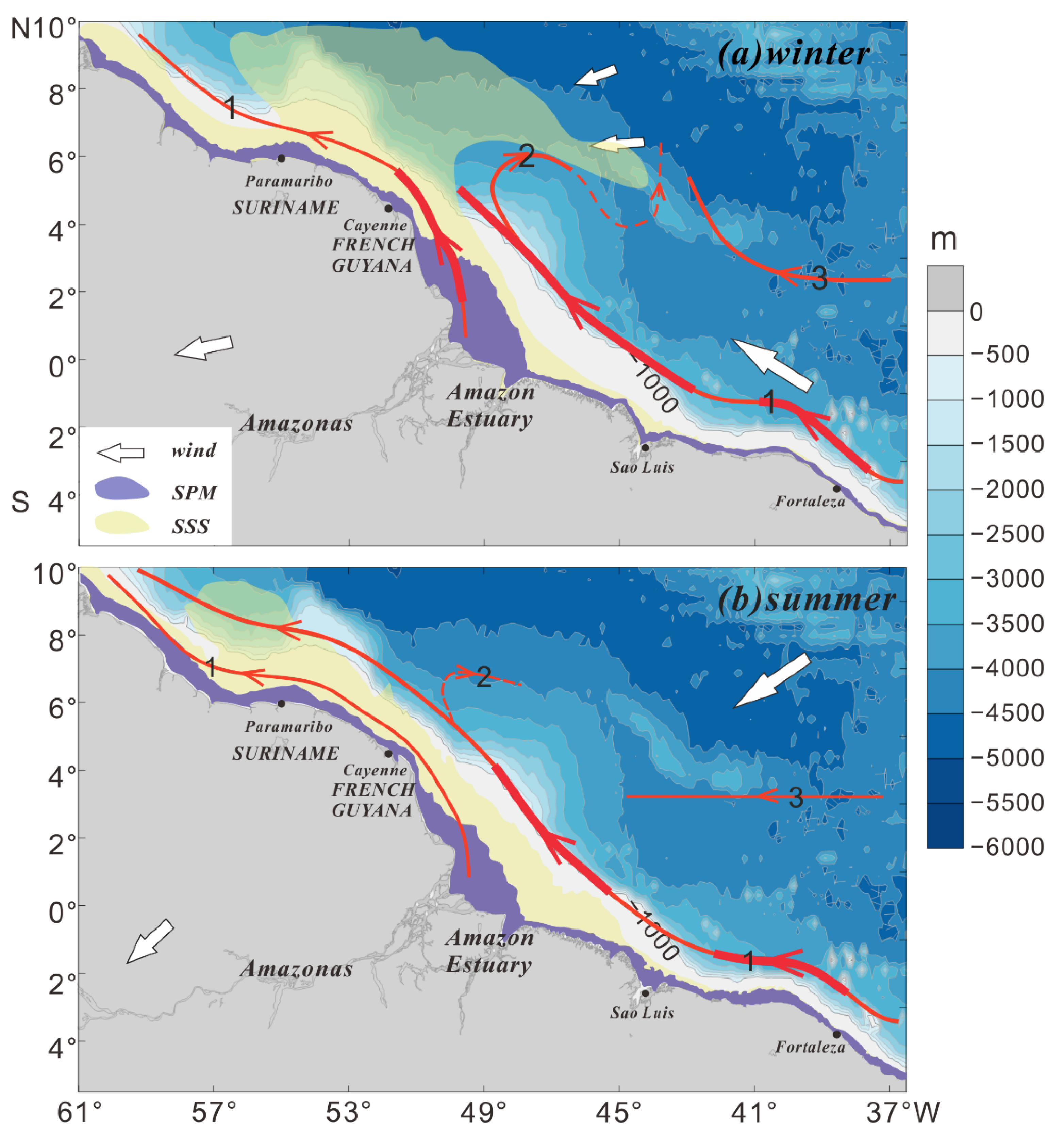
4.3. Two Patterns of River–Sea Interaction

Figure 9 basically indicates the mean state of the averaged distribution of SPM, the diffusion of diluted water from the Amazon River, the wind, and the current field based on winter semiannual and summer semiannual averaged distribution of the various elements. According to the trend and structure of these elements, typical contours of Rrs (0.025 sr−1) and SSS (30 PSU) were selected to represent boundary lines of the turbid region and diluted water, respectively. The results show the obvious spatial difference of the SPM distribution off the Amazon estuary, which was higher near shore and lower offshore (Figure 3). Most of the SPM that was carried by the river settled in the estuary area, and only a small amount was available to diffuse into the sea area far away from the estuary through hydrodynamic transport or resuspension [51].
The patterns for the winter and summer periods were similar in that they both showed the “filter effect” of the Amazon estuary (Figure 9). A series of physical, chemical, and biological processes takes place in the material carried by the river through the estuary under the actions of runoff, tidal currents, diluted water, salt water, and other factors. These processes lead to changes in the quantity and quality of the material carried by the river, such that the estuarine material flux to the ocean is not necessarily equal to the riverine material flux to the ocean. This process and the result of this change are the “filter effect” of the estuary. Based on this phenomenon, Wolanski and Gibbs [52] and Uncles and Stephens [53] made similar statements for the New Guinea River estuary and Tamar River, respectively. Li et al. [54] studied the “filter effect” of reservoirs in the Yangtze River basin with respect to the dissolved silicon flux to the sea. In this study, diluted water carried a large amount of SPM; however, under the sorting action of natural gravity, most of these materials diffused along the coasts, eventually being captured to remain on the continental shelf, while only a small amount diffused seaward. The direction of the current also reflected its interaction with the terrain. The NBC flowed around the continental shelf regularly in the northward direction, but flowed slowly on the continental shelf (Figure 9a). Liu et al. [55] conducted relevant experiments and confirmed that the current flowed along the isobaths in areas far away from the continental shelf and was blocked at the edge of the continental shelf, forming inertial boundary layers.
Nevertheless, there were also differences in the patterns of the dynamics between the winter and summer periods. During the summer period, the southeast trade wind was not significant, and the NECC, NSEC, and other ocean currents were restricted, leading to a weak development. Most of the SPM carried by river-diluted water diffused along the estuary to both sides of the coasts, with a small amount being distributed along the coast carried by the NBC, which was basically restricted to the estuarine shelf. In the winter period, the southeast trade wind gradually moved northward, which promoted the development of ocean currents, enhanced the NBC, and formed the NECC and NSEC, resulting in the enhanced diffusion of river-diluted water along the coasts and seaward. After diluted water diffused with the NBC to northwest of 6° N, it showed an obvious trend of spreading eastward with the NECC, and the total amount of the SPM in the estuary increased.
In addition, the influence of related rivers in the Amazon basin on estuarine sediment output is also significant. For example, the Pará River is a component of the Amazon hydrographic network in northern Brazil, and as for the Pará-Amazon estuarine system, there is an intense hydrodynamics sedimentation environment under the control of the wave action and tidal and river currents [56]. Prestes et al. [57,58,59] recorded current velocities in excess of 2.0 m/s in the Pará River, with the instantaneous discharges within the estuary of this river reaching 4.0 × 10⁵ m3/s. In that work, the multiyear averaged analysis weakened the short-term and instantaneous change in flow rate, making the Pará River show a maximum annual flow rate of 0.5 m/s (Figure 6). However, the curve of the northern coastline forced the fresh water from the rivers Amazon and Pará to run closer to the coast and be reinforced by the outflow [60].
In general, the river–sea interactions in estuaries worldwide present similar characteristics; however, there are some differences. Hopkins et al. [61] found that variations in the magnitude and direction of wind stress and wind-driven surface currents pushed freshwater from the Congo River northwestward or westward along the coasts towards the open South Atlantic Ocean. Apart from the runoff to the sea, the most important factors affecting the diffusion of the plume in the Mississippi River estuary were determined to be the magnitude and direction of the wind stress, whereas the tidal current had little effect [62]. For the Yangtze River estuary, suspended sediment transport was found to be mainly controlled by wind, current, tide, and upstream sediment transport, with the wind direction being the main influencing factor [63]. In this study, the current velocity was the main factor affecting the river–sea interaction off the Amazon estuary, with the strength of the trade winds promoting this interaction.
It is worth mentioning that, since the focus of this paper was to explore the variation of the multi-year average patterns of river–sea interactions, event-related fluctuations and high-frequency variability in the estuary area are not included in this work. In addition, the remote sensing data of typical tropical areas are greatly affected by clouds, so the short-term variability under extreme events is limited, especially close to the river mouth [4], which needs further study.

5. Conclusions

Based on the remote sensing data (2008–2017) of the MODIS aboard the Aqua satellite, in combination with data of the wind field, ocean current, SST, and water depth, this study explored the process and patterns of the river–sea interaction off the Amazon estuary. This was achieved by analyzing the distribution characteristics and diffusion of the SPM and river-diluted water in a mean state, which revealed the following conclusions.
The Amazon estuary has a “filter effect.” The SPM was generally derived from river-diluted water, and its distribution exhibited obvious spatial characteristics during the study period. The most significant characteristic was that the SPM was high near shore and low offshore. After diffusing to the estuary via the river-diluted water, most of the SPM remained on the shelf in a fan shape and was limited to the 200 m isobath. In addition, part of the SPM was distributed in the shallow water of the shelf along the coasts on both sides of the estuary.
It is clear that the current was the main factor affecting the diffusion of the SPM and diluted water off the Amazon estuary. Wind directly affected the velocity of the ocean currents; hence, ocean currents carried diluted water along the coasts and seaward. The interaction between the currents and the terrain limited the diffusion of the SPM.
Differences were observed in the river–sea interaction patterns off the Amazon estuary between the winter and summer periods. During the winter period, the southeast trade wind moved northward. The seaward diffusion of river-diluted water increased with the generation of ocean currents, the strengthening of the NBC, and the formation of the NECC and NSEC. However, the southeast trade wind was not significant; hence, the NECC, NSEC, and other ocean currents were not well generated during the summer period. The seaward diffusion trend of river-diluted water was not obvious. Furthermore, the diffusion ranges of the SPM and diluted water differed. Most of the SPM was captured by the continental shelf and remained in the estuarine area, thus limiting the diffusion distance and range. In contrast, diluted water had a longer and wider diffusion distance and range, respectively.
In summary, this study revealed the process and patterns of the river–sea interaction in the Amazon estuary, which could provide a reference for future research on the Amazon estuary and other large rivers worldwide.

Author Contributions

Conceptualization, D.Y., S.L., G.L., and Y.Z.; methodology, D.Y., S.L., G.L., and Y.Z.; software, G.L., Y.Z., and J.S.; validation, D.Y., S.L., and X.L.; investigation, D.Y., X.L., J.L., and X.W.; writing—original draft preparation, D.Y.; writing—review and editing, D.Y., S.L., G.L., Y.Z., J.S., X.L., and X.W.; project administration, S.L., G.L., X.L., J.L., and X.W.; funding acquisition, S.L. and G.L. All authors have read and agreed to the published version of the manuscript.

Funding

This research was jointly funded by the National Key R&D Program-Intergovernmental Key Special Project (No. 2017YFE0133500), the Qingdao Science and Technology Bureau Project—Development of Green Tide Disaster Prediction System in Qingdao Sea Area (19-6-1-77-nsh), the Taishan Scholar Project grant to G.L., and the National Natural Science Foundation of China (grants 41806072). Funding was also provided by the China Postdoctoral Science Foundation (grants 2019M652467) and Qingdao postdoctoral application research.

Institutional Review Board Statement

Not applicable.

Informed Consent Statement

Not applicable.

Data Availability Statement

MODIS data: NASA, https://www.nasa.gov (accessed on 13 October 2020); SSS data: Qingdao Blue Earth Big Data Technology Co., Ltd.; wind data: CCMP, http://www.remss.com/measurements/ccmp/ (accessed on 19 April 2019); ocean current data: SODA, https://www.atmos.umd.edu/~ocean/ (accessed on 19 April 2019); water depth data: Eptopo1, https://www.ngdc.noaa.gov/mgg/global/global.html (accessed on 1 February 2021).

Acknowledgments

The authors would like to thank the NASA MODIS Project for the production and distribution of MODIS data, the University of Maryland for the current data, and NOAA for the data on the water depth. The authors also thank the National Key R&D Program-Intergovernmental Key Special Project (2017YFE0133500) and the Taishan Scholar Project (GXLI) for the support. Thanks to the editors and three anonymous reviewers for the constructive comments on this manuscript.

Conflicts of Interest

The authors declare no conflict of interest.

References

  1. Pang, C.; Wang, F. The Distributing Features and Temporal Variability of Suspended Matter Concentration in the East China Sea. Studia Mar. Sin. 2004, 46, 22–31. [Google Scholar]
  2. Gensac, E.; Martinez, J.-M.; Vantrepotte, V.; Anthony, E.J. Seasonal and inter-annual dynamics of suspended sediment at the mouth of the Amazon river: The role of continental and oceanic forcing, and implications for coastal geomorphology and mud bank formation. Cont. Shelf. Res. 2016, 118, 49–62. [Google Scholar] [CrossRef]
  3. Villar, R.E.; Martinez, J.-M.; Texier, M.L.; Guyot, J.-L.; Fraizy, P.; Meneses, P.R.; Oliveira, E.D. A study of sediment transport in the Madeira River, Brazil, using MODIS remote-sensing images. J. S. Am. Earth Sci. 2013, 44, 45–54. [Google Scholar] [CrossRef]
  4. Hu, C.; Montgomery, E.T.; Schmitt, R.W.; Muller-Karger, F.E. The dispersal of the Amazon and Orinoco River water in the tropical Atlantic and Caribbean Sea: Observation from space and S-PALACE floats. Deep Sea Res. Part II Top. Stud. Oceanogr. 2004, 51, 1151–1171. [Google Scholar] [CrossRef]
  5. Filizola, N.; Guyot, J.L.; Wittmann, H.; Martinez, J.M.; Oliveira, E.D. The Significance of Suspended Sediment Transport Determination on the Amazonian Hydrological Scenario. In Sediment Transport in Aquatic Environments, 3rd ed.; Andrew, M., Ed.; IntechOpen: London, UK, 2011; Chapter 3; pp. 46–64. [Google Scholar]
  6. Le Bars, Y.; Lyard, F.; Jeandel, C.; Dardengo, L. The amandes tidal model for the Amazon estuary and shelf. Ocean Model. 2010, 31, 132–149. [Google Scholar] [CrossRef]
  7. Gibbs, R.J. Amazon River: Environmental Factors That Control Its Dissolved and Suspended Load. Science 1967, 156, 1734–1737. [Google Scholar] [CrossRef]
  8. Gibbs, R.J. Water chemistry of the Amazon River. Geochim. Cosmochim. Acta 1972, 36, 1061–1066. [Google Scholar] [CrossRef]
  9. Gibbs, R.J. Amazon River sediment transport in the Atlantic Ocean. Geology 1976, 4, 45–48. [Google Scholar] [CrossRef]
  10. Richey, J.E.; Meade, R.H.; Salati, E.; Devol, A.H.; Nordin, C.F.; Santos, U.D. Water Discharge and Suspended Sediment Concentrations in the Amazon River 1982–1984; John Wiley and Sons Ltd.: Hoboken, NJ, USA, 1986; Volume 22, pp. 756–764. [Google Scholar]
  11. Kineke, G.C.; Sternberg, R.W. Distribution of fluid muds on the Amazon continental shelf. Mar. Geol. 1995, 125, 193–233. [Google Scholar] [CrossRef]
  12. Lentz, S.J. The Amazon River Plume during Amasseds: Subtidal Current Variability and the Importance of Wind Forcing; John Wiley and Sons Ltd.: Hoboken, NJ, USA, 1995; Volume 100, pp. 2377–2390. [Google Scholar]
  13. Geyer, W.R.; Beardsley, R.C.; Lentz, S.J.; Candela, J.; Limeburner, R.; Johns, W.E.; Castro, B.M.; Soares, I.D. Physical oceanography of the Amazon shelf. Cont. Shelf. Res. 1996, 16, 575–616. [Google Scholar] [CrossRef]
  14. Kineke, G.C.; Sternberg, R.W.; Trowbridge, J.H.; Geyer, W.R. Fluid-mud processes on the Amazon continental shelf. Cont. Shelf. Res. 1996, 16, 667–696. [Google Scholar] [CrossRef]
  15. Park, E.; Latrubesse, E.M. Modeling suspended sediment distribution patterns of the Amazon River using MODIS data. Remote Sens. Environ. 2014, 147, 232–242. [Google Scholar] [CrossRef]
  16. Vantrepotte, V.; Gensac, E.; Loisel, H.; Gardel, A.; Dessailly, D.; Mériaux, X. Satellite assessment of the coupling between in water suspended particulate matter and mud banks dynamics over the French Guiana coastal domain. J. S. Am. Earth Sci. 2013, 44, 25–34. [Google Scholar] [CrossRef]
  17. Chérubin, L.M.; Richardson, P.L. Caribbean current variability and the influence of the Amazon and Orinoco freshwater plumes. Deep. Sea Res. Part I Oceanogr. Res. 2007, 54, 1451–1473. [Google Scholar] [CrossRef] [Green Version]
  18. SeaWiFS: The Effect of the Amazon on the Atlantic. Available online: https://svs.gsfc.nasa.gov/2078 (accessed on 18 February 2021).
  19. Gouveia, N.A.; Gherardi, D.F.M.; Wagner, F.H.; Paes, E.T.; Coles, V.J.; Aragão, L.E.O.C. The Salinity Structure of the Amazon River Plume Drives Spatiotemporal Variation of Oceanic Primary Productivity. J. Geophys. Res. Biogeosci. 2019, 124, 147–165. [Google Scholar] [CrossRef] [Green Version]
  20. Martinez, J.M.; Guyot, J.L.; Filizola, N.; Sondag, F. Increase in suspended sediment discharge of the Amazon River assessed by monitoring network and satellite data. Catena 2009, 79, 257–264. [Google Scholar] [CrossRef] [Green Version]
  21. Warrick, J.A.; Mertes, L.A.K.; Siegel, D.A.; Mackenzie, C. Estimating suspended sediment concentrations in turbid coastal waters of the Santa Barbara Channel with SeaWiFS. Int. J. Remote Sens. 2004, 25, 1995–2002. [Google Scholar] [CrossRef]
  22. Kowalczuk, P.; Stedmon, C.A.; Markager, S. Modeling absorption by CDOM in the Baltic Sea from season, salinity and chlorophyll. Mar. Chem. 2006, 101, 1–11. [Google Scholar] [CrossRef]
  23. Das, S.; Das, I.; Giri, S.; Chanda, A.; Maity, S.; Lotliker, A.A.; Kumar, T.S.; Akhand, A.; Hazra, S. Chromophoric Dissolved Organic Matter (CDOM) Variability Over The Continental Shelf of The Northern Bay of Bengal. Oceanologia 2017, 59, 271–282. [Google Scholar] [CrossRef]
  24. Harvey, E.T.; Kratzer, S.; Andersson, A. Relationships between colored dissolved organic matter and dissolved organic carbon in different coastal gradients of the Baltic Sea. Ambio 2015, 44, 392–401. [Google Scholar] [CrossRef] [Green Version]
  25. Kong, D.; Yang, H.; Wu, J. Optical absorption properties of chromophoric dissolvable organic matter in Changjiang Estuary. Mar. Environ. Sci. 2008, 27, 629–631. [Google Scholar]
  26. Reul, N.; Fournier, S.; Boutin, J.; Hernandez, O.; Maes, C.; Chapron, B.; Alory, G.; Quilfen, Y.; Tenerelli, J.; Morisset, S.; et al. Sea Surface Salinity Observations from Space with the SMOS Satellite: A New Means to Monitor the Marine Branch of the Water Cycle. Surv. Geophys. 2014, 35, 681–722. [Google Scholar] [CrossRef] [Green Version]
  27. Kuhn, C.; De Matos Valerio, A.; Ward, N.; Loken, L.; Sawakuchi, H.O.; Kampel, M.; Richey, J.; Stadler, P.; Crawford, J.; Striegl, R.; et al. Performance of landsat-8 and sentinel-2 surface reflectance products for river remote sensing retrievals of chlorophyll-a and turbidity. Remote Sens. Environ. 2019, 224, 104–118. [Google Scholar] [CrossRef] [Green Version]
  28. Atlas, R.M.; Ardizzone, J.V.; Hoffman, R.N.; Jusem, J.C. The cross-calibrated, multi-platform (CCMP) ocean surface wind product: Current status and plans. In Proceedings of the AGU Fall Meeting Abstracts, New Orleans, LA, USA, 1 December 2009; p. IN41B-06. [Google Scholar]
  29. Carton, J.A.; Giese, B.S. A Reanalysis of Ocean Climate Using Simple Ocean Data Assimilation (SODA). Mon. Weather Rev. 2008, 138, 2999–3017. [Google Scholar] [CrossRef]
  30. Duan, Y.; Liu, H.; Yu, W.; Hou, Y. The mean properties and variations of the Southern Hemisphere subpolar gyres estimated by Simple Ocean Data Assimilation (SODA) products. Acta Oceanol. Sin. 2016, 35, 8–13. [Google Scholar] [CrossRef]
  31. Liu, H.; Zhang, Q.; Duan, Y.; Hou, Y. The three-dimensional structure and seasonal variation of the North Pacific meridional overturning circulation. Acta Oceanol. Sin. 2011, 30, 33–42. [Google Scholar] [CrossRef]
  32. Lee, Z. Update of the Quasi-Analytical Algorithm (QAA_v6) [R/OL]. International Ocean Color Group Software Report. Available online: https://www.ioccg.org/groups/software.html (accessed on 3 April 2013).
  33. Lee, Z.; Carder, K.L.; Arnone, R.A. Deriving inherent optical properties from water color: A multiband quasi-analytical algorithm for optically deep waters. Appl. Opt. 2002, 41, 5755–5772. [Google Scholar] [CrossRef]
  34. Zheng, G.; Stramski, D.; Reynolds, R.A. Evaluation of the QAA Algorithm for Estimating the Inherent Optical Properties from Remote Sensing Reflectance in Arctic Waters. In Proceedings of the 2010 AGU Ocean Sciences Meeting, Washington, DC, USA, 7 January 2010. [Google Scholar]
  35. Lian-Bo, H.U.; Liu, Z.S. Deriving Absorption Coefficients from Remote Sensing Reflectance Using the Quasi-Analytical Algorithm (QAA) in the Yellow Sea. Period. Ocean. Univ. China 2007, 37 (Suppl. II), 154–160, (In Chinese with English abstract). [Google Scholar]
  36. Wang, Y.; Shen, F.; Sokoletsky, L.; Sun, X. Validation and Calibration of QAA Algorithm for CDOM Absorption Retrieval in the Changjiang (Yangtze) Estuarine and Coastal Waters. Remote Sens. 2017, 9, 1192. [Google Scholar] [CrossRef] [Green Version]
  37. Le, C.; Hu, C. A hybrid approach to estimate chromophoric dissolved organic matter in turbid estuaries from satellite measurements: A case study for Tampa Bay. Opt. Express 2013, 21, 18849. [Google Scholar] [CrossRef]
  38. Wang, M.; Shi, W. The NIR-SWIR combined atmospheric correction approach for MODIS ocean color data processing. Opt. Express 2007, 15, 15722–15733. [Google Scholar] [CrossRef] [PubMed] [Green Version]
  39. Vecchio, R.D.; Subramaniam, A. Influence of the Amazon River on the surface optical properties of the western tropical North Atlantic Ocean. J. Geophys. Res. 2004, 109, C11. [Google Scholar] [CrossRef]
  40. Wang, Z. Study on the Linkage of the Southern Hemisphere Extratropical Climate Variability to Two Types of ENSO and the Relationship between ENSO and SAM. Master′s Thesis, Shanghai Jiao Tong University, Shanghai, China, 2019. [Google Scholar]
  41. Liang, Y.-C.; Lo, M.-H.; Lan, C.-W.; Seo, H.; Ummenhofer, C.C.; Yeager, S.; Wu, R.-J.; Steffen, J.D. Amplified seasonal cycle in hydroclimate over the Amazon river basin and its plume region. Nat. Commun. 2020, 11, 1–11. [Google Scholar] [CrossRef] [PubMed]
  42. Muller-Karger, F.E.; McClain, C.R.; Richardson, P.L. The dispersal of the Amazon’s water. Nature 1988, 333, 56–59. [Google Scholar] [CrossRef]
  43. Silva, A.C.; Bourles, B.; Araujo, M. Circulation of the thermocline salinity maximum waters off the Northern Brazil as inferred from in situ measurements and numerical results. Ann. Geophys. 2009, 27, 1861–1873. [Google Scholar] [CrossRef] [Green Version]
  44. Grodsky, S.A.; Carton, J.A. Surface drifter pathways originating in the equatorial Atlantic cold tongue. Geophys. Res. Lett. 2002, 29, 621–624. [Google Scholar] [CrossRef] [Green Version]
  45. Arnault, S.; Thiria, S.; Crépon, M.; Kaly, F. A tropical Atlantic dynamics analysis by combining machine learning and satellite data. Adv. Space Res. 2020, 68, 467–486. [Google Scholar] [CrossRef]
  46. Johns, W.E.; Lee, T.N.; Schott, F.A.; Zantopp, R.J.; Evans, R.H. The North Brazil Current Retroflection: Seasonal Structure and Eddy Variability; John Wiley and Sons Ltd.: Hoboken, NJ, USA, 1990; Volume 95, pp. 22103–22120. [Google Scholar]
  47. Curtin, T.B.; Legeckis, R.V. Physical observations in the plume region of the Amazon River during peak discharge—I. Surface variability. Cont. Shelf. Res. 1986, 6, 31–51. [Google Scholar] [CrossRef]
  48. Meade, R.H.; Dunne, T.; Richey, J.E.; Santos, U.D.; Salati, E. Storage and remobilization of suspended sediment in the lower Amazon River of Brazil. Science 1985, 228, 488–490. [Google Scholar] [CrossRef] [Green Version]
  49. Kuehl, S.A.; Demaster, D.J.; Nittrouer, C.A. Nature of sediment accumulation on the Amazon continental shelf. Cont. Shelf. Res. 1986, 6, 209–225. [Google Scholar] [CrossRef]
  50. Nittrouer, C.A.; Curtin, T.B.; Demaster, D.J. Concentration and flux of suspended sediment on the Amazon continental shelf. Cont. Shelf. Res. 1986, 6, 151–174. [Google Scholar] [CrossRef]
  51. Wang, W. Study on the Suspended Matter’s Distribution from Remote Sensing Retrieval and its Movement Mechanisms in the Surface Layer of the East China Seas. Master’s Thesis, Ocean University of China, Qingdao, China, 2008. [Google Scholar]
  52. Wolanski, E.; Gibbs, R.J. Flocculation of suspended sediment in the Fly River estuary, Papua New Guinea. J. Coastal Res. 1995, 40, 321–337. [Google Scholar]
  53. Uncles, R.J.; Stephens, J.A. Nature of the Turbidity Maximum in the Tamar Estuary, U.K. Estuar. Coast. Shelf Sci. 1993, 36, 413–431. [Google Scholar] [CrossRef]
  54. Li, M.; Sun, Q.; Wang, H.; Liu, Y.; Lai, X. The Filter Effect of Big Reservoirs on Dissolved Silicate in the Yangtze River Drainage Basin. J. Lake Sci. 2014, 26, 505–514. [Google Scholar]
  55. Liu, Q.; Jia, F.; Wang, P. Laboratory Modelling of Topographic Effects on the Oceanic Current. Theor. Appl. Mec. 1981, 6, 611–618. [Google Scholar]
  56. Costa, M.; Rollnic, M.; Silveira, O.; Miranda, A.; Santos, R. Morphological and sedimentological processes of an Amazon Estuary, Maguari River (Pará—Northern Brazil). J. Coastal Res. 2013, 165, 1110–1115. [Google Scholar] [CrossRef]
  57. Prestes, Y.O.; Rollnic, M.; Silva, M.S.; Rosario, R.P. Volume transport in the tidal limit of the Pará River, Brazil. In Proceedings of the 17th physics of estuaries and coastal seas conference, Porto de Galinhas, Pernambuco, Brazil, 19–23 October 2014. [Google Scholar]
  58. Prestes, Y.O.; Silva, A.C.; Rollnic, M.; Rosario, R.P. The M2 and M4 tides in the Pará River Estuary. Trop. Oceanogr. 2017, 45, 26–37. [Google Scholar]
  59. Prestes, Y.O.; da Costa, B.T.A.; da Silva, A.C.; Rollnic, M. A discharge stationary model for the Pará-Amazon estuarine system. J. Hydrol-Reg Stud. 2020, 28, 100668. [Google Scholar] [CrossRef]
  60. Magliocca, A. Some chemical aspects of the marine environment off the amazon and pará rivers, brazil. Braz. J. Oceanogr. 1971, 20, 61–84. [Google Scholar] [CrossRef]
  61. Hopkins, J.; Lucas, M.; Dufau, C.; Sutton, M.; Stum, J.; Lauret, O.; Channelliere, C. Detection and variability of the Congo River plume from satellite derived sea surface temperature, salinity, ocean colour and sea level. Remote Sens. Environ. 2013, 139, 365–385. [Google Scholar] [CrossRef]
  62. Walker, N.D. Satellite assessment of Mississippi River plume variability: Causes and predictability. Remote Sens. Environ. 1996, 58, 21–35. [Google Scholar] [CrossRef]
  63. Xue, W.; Qiao, L.; Zhong, Y.; Xue, C.; Chen, S.; Li, S.; Liu, P.; Gao, F. Multiple Timescale Variation in Concentration of Surface Suspended Sediment in Changjiang River Estuary. Oceanol. Et Limnol. Sin. 2019, 50, 1002–1013. [Google Scholar]
Figure 1. Bird’s-eye-view image of the study area in the Amazon estuary (ETOPO1 Global Relief Model, https://www.ngdc.noaa.gov/mg/global/global.html (accessed on 1 February 2021)). M and N are two transects perpendicular to and parallel to the shoreline, respectively, which will be discussed in the following sections.
Remotesensing 14 01022 g001
Figure 2. The fitting relationship image between SSS and aCDOM (with 95% confidence bounds). The horizontal axis represents aCDOM (unit: m−1), whereas the ordinate represents the measured salinity value (unit: PSU).
Remotesensing 14 01022 g002
Figure 3. The deviation between the monthly average and annual average remote-sensing reflectance (Rrs) at the 555 nm band over 10 years off the Amazon estuary (2008–2017). The purple contour lines from the estuary to the sea are the 50 m, 200 m, and 2000 m isobaths. (al) correspond to the winter period (June–November) and summer period (December–May) in the southern hemisphere, respectively (unit: sr−1). Transects M and N are indicated in (a).
Remotesensing 14 01022 g003
Figure 4. Monthly average SSS over 10 years off the Amazon estuary (2008–2017). The grey contour lines from the estuary to the sea are the 50 m, 200 m, and 2000 m isobaths. (al) correspond to the winter period (June–November) and summer period (December–May) in the southern hemisphere, respectively (unit: PSU). Transects M and N are indicated in (a).
Remotesensing 14 01022 g004
Figure 5. Monthly average wind field over 10 years in the study area off the Amazon estuary (2008–2017). (al) correspond to the winter period (June–November) and summer period (December–May) in the southern hemisphere, respectively (unit: m/s).
Remotesensing 14 01022 g005
Figure 6. Monthly average flow field over 10 years in the sea area of the Amazon estuary (2008–2017). (al) correspond to the winter period (June–November) and summer period (December–May) in the southern hemisphere, respectively (unit: m/s). Transects M and N are indicated in (a).
Remotesensing 14 01022 g006
Figure 7. Ten-year averaged monthly variations of various elements along transect M. (a) Water remote-sensing reflectance (Rrs, to represent the SPM; unit: lg(sr−1)); (b) sea surface salinity (SSS; unit: PSU); (c) sea surface temperature (SST; unit: °C); (d) ocean current velocity (unit: m/s). The ordinate is the month (January–December) and the abscissa is the longitude.
Remotesensing 14 01022 g007
Figure 8. Ten-year averaged monthly variations of various elements along transect N. (a) Water remote-sensing reflectance (Rrs, to represent the SPM; unit: lg(sr−1)); (b) sea surface salinity (SSS; unit: PSU); (c) sea surface temperature (SST; unit: °C); (d) ocean current velocity (unit: m/s). The ordinate is the month (January–December) and the abscissa is the longitude.
Remotesensing 14 01022 g008
Figure 9. The river–sea interaction patterns off the Amazon estuary. (a) Winter semiannual pattern; (b) summer semiannual pattern. The contour map and gray lines are the water depth and isobaths. The purple region and yellow region represent the Rrs and SSS, respectively. The red arrows represent the ocean currents and the thickness represents the flow velocity. The number 1 represents the NBC, which exists throughout the year and mainly restricts the seaward diffusion of SPM. The number 2 represents the NECC, which has obvious seasonal variation characteristics. The number 3 represents the NSEC, which supplies the NECC. The dashed red lines indicate the seasonal differences in development. The white arrows indicate the wind directions, whose size distinguishes the wind speed.
Remotesensing 14 01022 g009
Publisher’s Note: MDPI stays neutral with regard to jurisdictional claims in published maps and institutional affiliations.

