A Novel High-Squint Spotlight SAR Raw Data Simulation Scheme in 2-D Frequency Domain

Abstract

Raw data simulation is the front-end work of synthetic aperture radar (SAR), which is of great significance. For high-squint spotlight SAR, the frequency domain simulation algorithm is invalid because of the range-azimuth coupling effect. In order to realize high-squint spotlight SAR raw data simulation in the frequency domain, an algorithm based on coordinate transformation and non-uniform fast Fourier transform (NUFFT) is proposed. This algorithm generates broadside raw data using a two-dimensional (2-D) frequency simulation algorithm; then, coordinate transformation is used by analyzing the characteristics of broadside and high-squint spotlight SAR. After coordinate transformation, NUFFT is carried out to realize the coupling relation in the 2-D frequency domain. Since the coordinate transformation ignores the influence of range walk, the range walk is compensated after NUFFT. As a result, compared with the traditional squint spotlight SAR frequency domain simulation algorithm, the proposed algorithm can improve the accuracy of point and distributed target imaging results, and the efficiency of the proposed algorithm can be significantly improved in contrast the traditional time domain algorithm.

1. Introduction

Synthetic aperture radar (SAR) is an active imaging technology, based on microwaves, which has the ability to observe the Earth, all day and during all weathers. SAR can be operated in a number of different modes, such as stripmap, spotlight, scan and terrain observation by progressive scan (TOPS) [1,2,3,4,5,6,7]. Each mode has its own strengths and weaknesses. For the spotlight SAR mode, it steers the beam over the full acquisition time to illuminate the same area (a spot on the ground), so as to improve the azimuth resolution. Due to the mobility of SAR platforms, a high or low squint angle always exists [8,9]. Therefore, squint spotlight SAR has been widely used in high-resolution Earth-observation missions.

With the further development of SAR technology, raw data simulation has become an important research direction. Raw data simulation is helpful to verify the performance of a SAR system, and the system parameters can be optimized after simulation [10,11,12,13,14,15,16]. The time domain algorithm and the frequency domain algorithm are two ways of performing SAR raw data simulations. The high computational complexity of the time domain algorithm makes it difficult to simulate large scenes. Some researchers have proposed several time domain raw data simulation acceleration algorithms. Fu et al. used a graphics processing unit (GPU) to accelerate the time domain raw data simulation of high-squint spotlight SAR [17], and Zhang et al. also used GPU to accelerate raw data simulation of multiple-mode SAR [18,19,20]. However, these algorithms have high hardware requirements and the effect of acceleration is limited [21]. Therefore, it is necessary to research the frequency domain algorithm. In [22,23,24,25,26,27,28,29,30], Franceschetti et al. described the methods of frequency domain raw data simulation in particular. Such a simulator first builds a geometric model, and then, the scattering coefficient is calculated based on an asymptotic evaluation of SAR unit response. Finally, the data are processed in the two-dimensional (2-D) frequency domain to obtain the final raw data. The proposal of this direction is a significant milestone in the development of SAR raw data simulations. Subsequently, Franceschetti et al. proposed a method of spotlight SAR raw data simulation in the frequency domain. This method can simulate the range migration and the space-variant feature, andsimulation results verified the correctness of the algorithm. However, all the above methods mainly focus on the broadside mode. Wang et al. proposed a method to solve squint spotlight SAR raw data simulations [31]. It uses optical principles to efficiently calculate the interpolation results. Diao and Xu presented an efficient method for squint mode SAR raw data simulation, based on scaled Fourier transform (SCFT) in [32]. These methods, however, are only applicable to the case of small-squint spotlight SAR. In recent years, Li et al. proposed a method based on sub-aperture Keystone transform for squint SAR with a curved trajectory [33]. Although this method can accurately simulate the original raw data of extended scenes for high-squint SAR mounted on a maneuvering platform, its efficiency is much lower than 2-D frequency domain raw data simulation algorithms.

In order to precisely and efficiently calculate the high-squint raw data in the 2-D frequency domain, this work developed an algorithm based on coordinate transformation and non-uniform fast Fourier transform (NUFFT). First, due to the simplicity of the broadside SAR geometric model, calculating the broadside SAR raw data in the 2-D frequency domain was uncomplicated. The key to this algorithm was how to convert the raw data of broadside SAR to be equivalent to that of a high-squint SAR, and this problem can be solved by coordinate transformation. Then, in the process of coordinate transformation, interpolation was used to simulate the coupling of the azimuth and range. Because of the complexity of interpolation operations in data processing, we used the NUFFT instead of interpolation and fast Fourier transform (FFT). Finally, we simulated the linear range walk of high-squint SAR in the range frequency domain. This algorithm only required complex multiplications, and it was suitable for the characteristics of high-squint spotlight SAR raw data.

This article is organized as follows. In Section 2, the spotlight SAR geometric model and the broadside SAR raw data simulations in the frequency domain are introduced; more importantly, the coordinate transformation method and the application of NUFFT in this algorithm are described. In Section 3, some simulation and imaging results are shown. Moreover, the computational complexity of the algorithm is analyzed. In Section 4, we address relevant discussions and analyze the experimental results. Finally, some conclusions are reported in Section 5.

2. Models and Methods

2.1. Models

The geometries of broadside and high-squint spotlight SAR are shown in Figure 1, where the origin of the coordinate system is located at scene center O, and the X, Y and Z axes represent the azimuth, range, and geocentric directions, respectively. $R_c$ is the mid-range coordinate. $R_{start}$ and $R_{end}$ are the target-to-antenna distances at the beginning and end of SAR operations, r is the distance from the sensor to the center of the scene on the Zero-Doppler plane. As can be seen in Figure 1, the difference between the broadside and the high-squint is the look angle of the platform. However, the range-azimuth coupling effect is inegligible due to the squint angle. The signal model of the broadside and high-squint SAR are introduced in what follows.

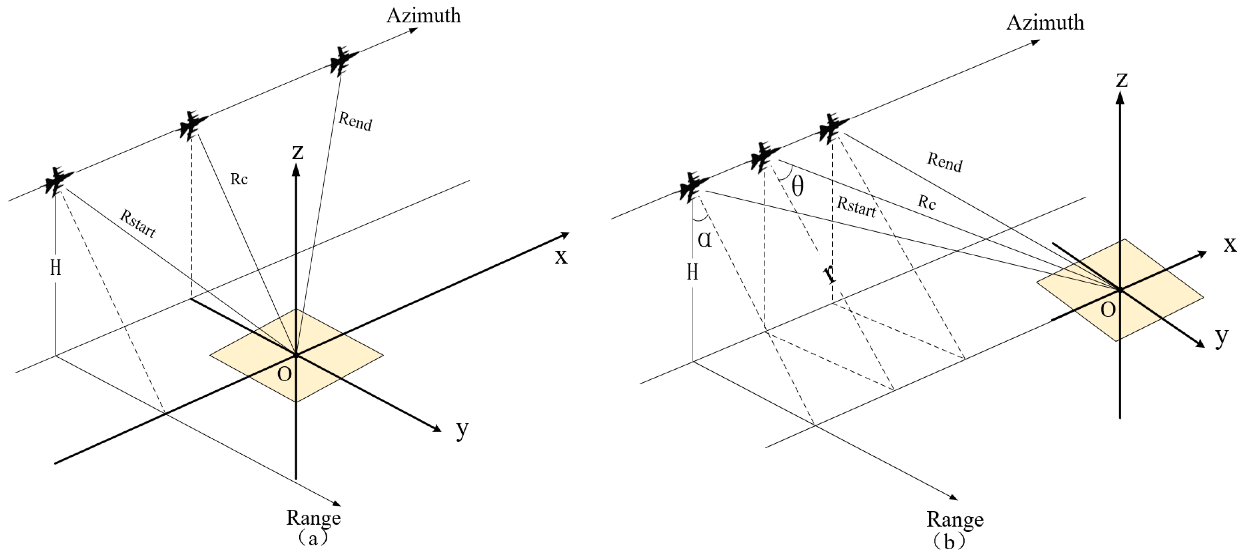
2.1.1. Broadside SAR

In reference to Figure 1a, the slant range distance between the radar and the target (x, y) in the case of broadside SAR is:

$$R\left(t_a\right)=\sqrt{{\left(v{t}_a-x\right)}^2+{\left(R_c-y\right)}^2-2\left(R_c-y\right)\left(v{t}_a-x\right)}$$

(1)

where v is the SAR sensor’s velocity and $t_a$ is the azimuth slow time. Then, the demodulated raw data can be expressed as:

$$S\left(t,t_a\right)=rect\left(\frac{t-\frac{2R\left(t_a\right)}{c}}{Tr}\right)·exp\left(-j\frac{4\pi R\left(t_a\right)}{\lambda }\right)·exp\left(-j\pi Kr{\left(t-\frac{2R\left(t_a\right)}{c}\right)}^2\right)$$

(2)

where t is the fast time, λ is the wavelength, Kr is the frequency modulation rate of the transmitted signal, Tr is the signal pulse width, and c is the propagation velocity of light.

The 2-D frequency spectrum of the scene raw signal is:

$$\begin{array}{c}S\left(f_r,f_a\right)={\displaystyle \iint }dxdy\sigma \left(x,y\right)·H_0\left(f_r,f_a\right)\\ \hspace{1em}=W\left(f_r\right)·exp\left(-j\frac{\pi f_r{}^2}{Kr}\right)·exp\left(-2j\pi \frac{x}{v}{f}_a\right)\\ \times exp\left(-4j\pi y\sqrt{{\left(\frac{f_c+f_r}{c}\right)}^2-{\left(\frac{f_a}{2v}\right)}^2}\right)\end{array}$$

(3)

where $\sigma \left(x,y\right)$ is the scattering coefficient of the scene and $W(·)$ is the envelopment of the transmitted signal window function after Fourier transform. $f_r$ is the range frequency, $f_a$ is the azimuth frequency, and $f_c$ is the carried frequency.

A flow chart of the frequency domain raw data simulation algorithm is shown in Figure 2. First, 2-D Fourier transform is performed according to scattering coefficient $\sigma \left(x,y\right)$, and then the raw data are calculated based on Equation (3). Finally, we determine the inverse Fourier transform using the data.

2.1.2. High-Squint SAR

With reference to Figure 1b, the slant range distance between the radar and the target $\left(x,y\right)$ in the case of high-squint SAR is:

$$R{\left(t_a\right)}^{\prime }=\sqrt{{\left(v{t}_a-x\right)}^2+{\left(R_c-y\right)}^2-2\left(R_c-y\right)\left(v{t}_a-x\right)sin\theta }$$

(4)

where $\theta$ is the center squint angle. In order to better analyze the distance characteristics in the case of squint, Equation (4) is expanded using the Taylor series at the central illuminated time:

$$\begin{array}{l}R{\left(t_a\right)}^{\prime }=R\left(t_a\right)-v·sin\theta ·\left(t_a-t_0\right)\\ +\frac{1}{2}·\frac{v^{2}co{s}^2\theta }{R\left(t_0\right)}{\left(t_a-t_0\right)}^2\\ +\frac{1}{2}·\frac{v^{3}sin\theta co{s}^2\theta }{R^2\left(t_0\right)}{\left(t_a-t_0\right)}^3+\cdots \\ =R\left(t_a\right)+X_1+X_2+X_3\end{array}$$

(5)

Equation (5) consists of range walk, $X_1=-v·sin\theta ·\left(t_a-t_0\right)$, range curvature, $X_2=\frac{1}{2}·\frac{v^{2}co{s}^2\theta }{R\left(t_0\right)}{\left(t_a-t_0\right)}^2$, and higher order terms, $X_3=\frac{1}{2}·\frac{v^{3}sin\theta co{s}^2\theta }{R^2\left(t_0\right)}{\left(t_a-t_0\right)}^3+\cdots$. The range walk is larger than the range curvature, and the range curvature is larger than the higher order terms. However, when the squint angle exists, the higher order terms cannot be ignored in the frequency domain raw data simulation. Therefore, the error increases rapidly with an increase in squint angle. Assuming that $\mathsf{\Delta }\psi /y$ represents the error, we can obtain:

$$\mathsf{\Delta }\psi /y=\left(R{\left(t_a\right)}^{\prime }-R\left(t_a\right)\right)/y$$

(6)

The frequency domain raw data simulation algorithm is suitable for large scene simulations in the case of limited time. However, in Figure 1a, there is a high-squint angle in the SAR system; according to Equations (2) and (5), the transfer function of the SAR system is related to the slant range distance. Moreover, Equation (6) reveals that when the squint angle increases, the error will increase exponentially; thus, the raw data have spatial variability, and cannot be directly calculated in a 2-D frequency. Therefore, the frequency domain raw data simulation algorithm is invalid when a squint angle exists.

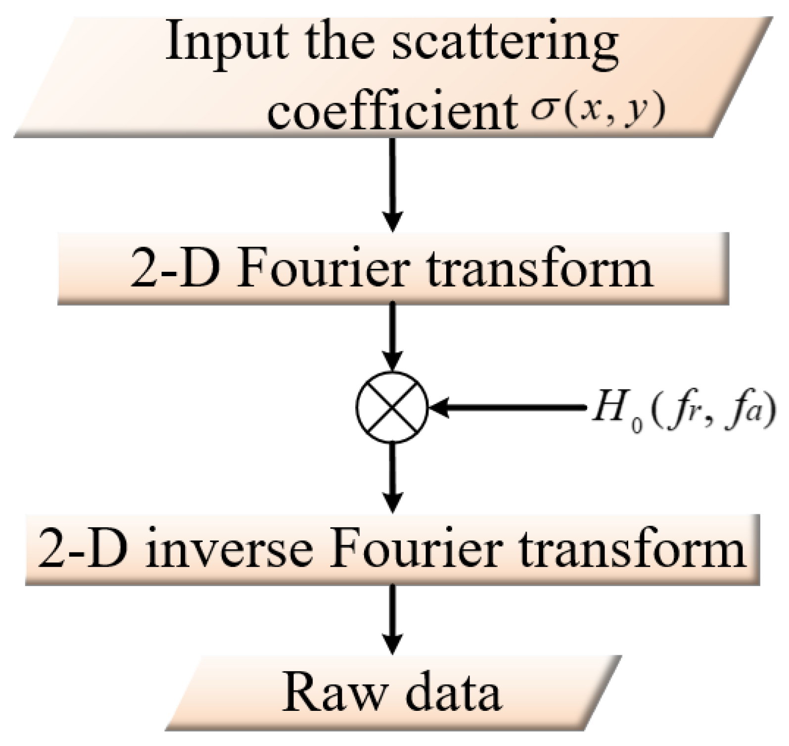
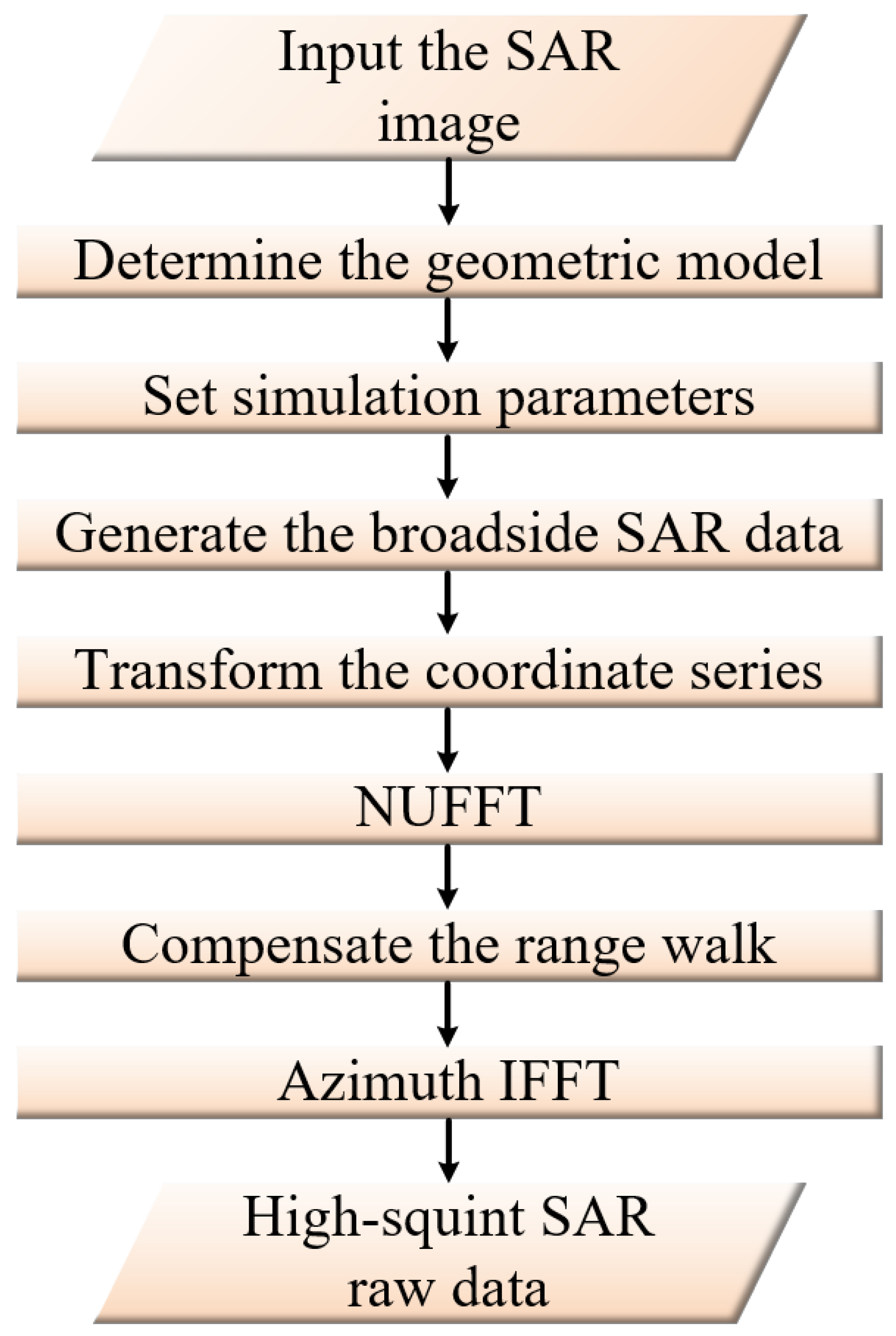
2.2. Methods

In order to solve the problem that the frequency domain raw data simulation algorithm is invalid in the case of high-squint SAR, an algorithm based on coordinate transformation and NUFFT was proposed. Due to the differences in the geometric model between broadside and high-squint SAR, we first generated broadside raw data using 2-D frequency simulation algorithm. To simulate the characteristics of high-squint SAR, a new approach based on coordinate transformation and NUFFT is presented in this section.

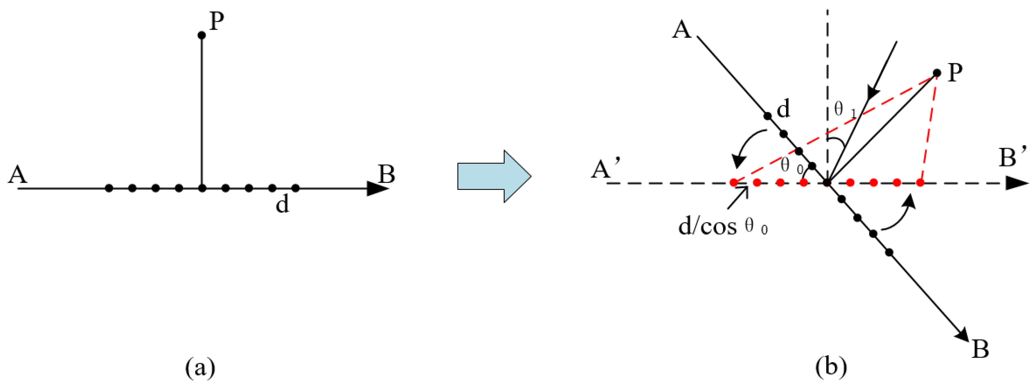
2.2.1. Coordinate Transformation

Figure 3a represents the geometric diagram between the platform and target, $AB$ denotes the motion trajectory array of the platform, and $d$ is the distance between two adjacent array elements. However, Figure 3a shows a geometric diagram of broadside SAR. To get the raw data of the high-squint SAR, rotating the coordinate series is a new way to address the problem of frequency domain raw data simulation. In an equivalent geometric diagram, depicted in Figure 3b, $A\prime B\prime$ is the motion trajectory array of the platform after coordinate transformation, and ${\theta }_0$ is the projection angle. As such, the distance between two adjacent array elements is changed to $d/cos{\theta }_0$. To explore the difference between motion trajectory arrays $AB$ and $A\prime B\prime$, the derivation process is shown as follows.

Assuming that the incident angle is ${\theta }_1$, the signal received by different coordinate series can be expressed as:

$$S_{AB}\left(t,n\right)=s\left(t\right)·exp(j{\phi }_0+j\frac{4\pi }{\lambda }nd\mathit{sin}\left({\theta }_1-{\theta }_0\right)$$

(7)

$$S_{A^{\prime }{B}^{\prime }}\left(t,n\right)=s\left(t\right)·exp\left(j{\phi }_0+j\frac{4\pi }{\lambda }n\frac{d}{\mathit{cos}{\theta }_0}sin{\theta }_1\right)$$

(8)

$$n\in \left[-\frac{\left(N-1\right)}{2},\frac{\left(N-1\right)}{2}\right]$$

(9)

where $s\left(t\right)$ is the amplitude of the signal and ${\phi }_0$ is the phase of the received signal. In Equation (9), $N$ is the serial number of samples.

Assuming that ${\theta }_1\approx {\theta }_0$, the following approximation can be used in this case:

$$sin{\theta }_1-sin{\theta }_0\approx \mathit{sin}\left({\theta }_1-{\theta }_0\right)\mathit{cos}{\theta }_0$$

(10)

According to Equation (10), the signal in Equation (8) can be rewritten as:

$$S_{A^{\prime }{B}^{\prime }}=S\left(t\right)·exp\left(j{\phi }_0+j\frac{4\pi }{\lambda }n\frac{d}{\mathit{cos}{\theta }_0}sin{\theta }_1-j\frac{4\pi }{\lambda }n\frac{d}{\mathit{cos}{\theta }_0}sin{\theta }_0\right)$$

(11)

where $-j\frac{4\pi }{\lambda }n\frac{d}{\mathit{cos}{\theta }_0}sin{\theta }_0$ is the order of the range walk, and this order is considered in Section 2.2.3. Then we can obtain:

$$S_{AB}\left(t,k\right)=S\left(t\right)·exp\left(j{\phi }_0\right)\delta (k-\frac{2Nd\mathit{sin}\left({\theta }_1-{\theta }_0\right)}{\lambda })$$

(12)

$$S_{A^{\prime }{B}^{\prime }}\left(t,k\right)=S\left(t\right)·exp\left(j{\phi }_0\right)\delta (k-\frac{2\frac{d}{\mathit{cos}{\theta }_0}N(\mathit{sin}{\theta }_1-\mathit{sin}{\theta }_0)}{\lambda })$$

(13)

Equations (12) and (13) are obtained by taking the Fourier transform with respect to the azimuth from Equations (7) and (12). Additionally, the Doppler frequency is changed as follows:

$$f_{AB}=\frac{d·PRF}{\lambda }\mathit{sin}\left({\theta }_1-{\theta }_0\right)$$

(14)

$$f_{A^{\prime }{B}^{\prime }}=\frac{d·PRF}{\mathit{cos}{\theta }_0·\lambda }(\mathit{sin}{\theta }_1-\mathit{sin}{\theta }_0)$$

(15)

where $PRF$ is the pulse repetition frequency, $f_{AB}$ is the azimuth frequency without the range walk order of motion trajectory array $AB$, and $f_{A^{\prime }{B}^{\prime }}$ is the azimuth frequency of the motion trajectory array $A\prime B\prime$. According to Equations (12)–(15), we have:

$$S_{AB}{\left(t,k\right)}^{\prime }=S\left(t\right)·exp\left(j{\phi }_0\right)\delta \left(k-2N\frac{f_{AB}}{PRF}\right)$$

(16)

$$S_{A^{\prime }{B}^{\prime }}{\left(t,k\right)}^{\prime }=S\left(t\right)·exp\left(j{\phi }_0\right)\delta \left(k-2N\frac{f_{A^{\prime }{B}^{\prime }}}{PRF}\right)$$

(17)

Observing the equations above, it is obvious that the differences in Equations (16) and (17) are only between $f_{AB}$ and $f_{A^{\prime }{B}^{\prime }}$. In order to eliminate the difference from motion trajectory arrays $AB$ and $A\prime B\prime$, we only need to consider the difference between $f_{AB}$ and $f_{A^{\prime }{B}^{\prime }}$. Let

$$f_{AB}{}^{\prime }=\frac{f_{AB}}{\mathit{sin}{\theta }_1-\mathit{sin}{\theta }_0}\mathit{cos}{\theta }_0\mathit{sin}\left({\theta }_1-{\theta }_0\right)=\frac{d·PRF}{\lambda }\mathit{sin}\left({\theta }_1-{\theta }_0\right)$$

(18)

According to Equation (17), we obtain:

$$\mathit{sin}{\theta }_1=\frac{\lambda f_{A\prime B\prime }{}^{\prime }}{v}+\mathit{sin}{\theta }_0$$

(19)

Then, $\mathit{sin}\left({\theta }_1-{\theta }_0\right)$ can be expressed as:

$$\begin{array}{l}\mathit{sin}\left({\theta }_1-{\theta }_0\right)=\mathit{sin}{\theta }_1\mathit{sin}{\theta }_0-\mathit{cos}{\theta }_1\mathit{cos}{\theta }_0\\ =\mathit{cos}{\theta }_0\left(\frac{\lambda f_{AB}}{v}+\mathit{sin}{\theta }_0\right)-\mathit{sin}{\theta }_0\sqrt{1-{\left(\frac{\lambda f_{AB}}{v}+\mathit{sin}{\theta }_0\right)}^2}\end{array}$$

(20)

Substituting (20) into (18), $f_{A\prime B\prime }{}^{\prime }$ can be rewritten as:

$$f_{AB}{}^{\prime }=\frac{d·PRF}{\lambda }(\mathit{cos}{\theta }_0\left(\frac{\lambda f_{AB}}{v}+\mathit{sin}{\theta }_0\right)-\mathit{sin}\theta \sqrt{1-{\left(\frac{\lambda f_{AB}}{v}+\mathit{sin}{\theta }_0\right)}^2})$$

(21)

The relevance between $f_{AB}{}^{\prime }$ and $f_{AB}$ is shown in Equation (21); after simplifying this equation and the equivalent substitution, we can obtain the following equation according to the “go-stop-go” assumption.

$$\begin{array}{l}\frac{f_a^{\prime }}{\mathit{cos}\theta }=(f_a+\frac{2v\mathit{sin}{\theta }_0}{c}\left(f_c+f_r\right)\\ -\mathit{tan}{\theta }_0\sqrt{{\left(\frac{2v}{c}\left(f_c+f_r\right)\right)}^2-{\left(f_a+\frac{2v\mathit{sin}{\theta }_0}{c}\left(f_c+f_r\right)\right)}^2}\\ =\left(f_a+f_{dc}\right)-\mathit{tan}\theta \sqrt{{\left(\frac{2v}{c}\left(f_c+f_r\right)\right)}^2-{\left(f_a+f_{dc}\right)}^2})\end{array}$$

(22)

with

$$f_{dc}=(2v\mathit{sin}{\theta }_0/c)\left(f_c+f_r\right)$$

(23)

Equation (22) is the frequency after coordinate transformation. Substituting (22) into (3), we can obtain:

$$\begin{array}{l}S\left(f_r,f_a\prime \right)=W_r\left(f_r\right)\\ \times \mathit{exp}\left(-\frac{j\pi f_r{}^2}{\gamma }\right)\mathit{exp}\left(-\frac{2j\pi (f_a^{\prime }+f_{dc})\left(R_0\mathit{sin}{\theta }_0+v{t}_c\right)}{v}\right)\\ \times exp(-4j\pi R_0\mathit{cos}{\theta }_0\sqrt{{\left(\frac{f_c+f_r}{c}\right)}^2-{\left(\frac{f_a^{\prime }+f_{dc}}{2v\mathit{cos}{\theta }_0}\right)}^2})\end{array}$$

(24)

The above equations describe the relevance of the azimuth frequency before and after coordinate transformation. Equation (24) is the 2-D frequency spectrum of the scene raw signal after coordinate transformation. The process from Equation (3) to Equation (24) requires interpolation, butmotion trajectory array $A\prime B\prime$ is non-uniform. Among the interpolation methods, the great majority of methods are not suitable for this situation. Those that are generally used may reduce computational efficiency and even cause deviations. Therefore, it is important to use a suitable method.

2.2.2. NUFFT

NUFFT is not a standard fast Fourier transform algorithm, but it is suitable for interpolation calculations of non-uniform data. According to Section 2.2.1, the array is non-uniform after coordinate transformation. In this case, NUFFT can not, only complete interpolation, but also complete azimuth Fourier transform. This operation is convenient to complete subsequent operations in the azimuth time domain, so the algorithm structure is optimized, and the efficiency is improved [34,35,36].

There are three kinds of NUFFTof interest: type-1 is non-equispaced data (NED) NUFFT, in which the spatial samples are located irregularly, and the spectral samples regular. Type-2 is non-equispaced result (NER) NUFFT, where the spatial samples are located regularly, and the spectral samples irregularly. In type-3, both the spatial and spectral samples are located irregularly. According to the process of coordinate transformation, NED NUFFT is suitable for this approach.

The NED NUFFT of samples ${\left\{Z_l\right\}}_{l=1}^M$, located at non-equispaced points, ${\left\{x_l\right\}}_{l=1}^M$, and evaluated on an equispaced grid, is defined as:

$${\widehat{Z}}_k={{\displaystyle \sum }}_{l=1}^M{Z}_{l}exp\left(-j2\pi x_l\frac{k}{N}\right), k=-\frac{N}{2},\cdots , \frac{N}{2}-1$$

(25)

In Equation (25), if $M=N, x_l=l$, the NUFFT will become a uniform Fourier transform. According to the above process, the NED NUFFT uses a Fourier series, which is truncated, to approximate signal $exp\left(j\xi x\right)$ with Gaussian kernel $exp\left(-b{x}^2\right)$.

$$\mathsf{\phi }\left(x\right)=exp\left(-b{x}^2\right)exp\left(j\xi x\right)$$

(26)

where $b$ is a coefficient of the Gaussian kernel. After derivation, the following equation is obtained:

$${\widehat{Z}}_k=\frac{{\left(2\pi \right)}^{-1/2}}{\omega \left(\frac{2\pi k}{\xi N}\right)}{{\displaystyle \sum }}_{\left|m\right|\le K}{{\displaystyle \sum }}_{l=1}^M{Z}_l\widehat{\varnothing }\left(\xi x-m\right)exp\left(-j2\pi mk/\xi N\right), k=-\frac{N}{2},\cdots , \frac{N}{2}-1$$

(27)

where $\omega (·)$ is the window function, $m$ is an independent variable regarding signal, and $\xi$ can be interpreted as an oversampling factor. Generally, $\xi =2$. $\widehat{\varnothing }$ represents the interpolation function.

According to Equations (26) and (27),functions of $exp\left(j\xi x\right)$ can be approximated by the finite order of $\mathsf{\phi }\left(x\right)$. The steps of the NUFFT algorithm according to [37] are:

(1)

The window function is used to process the raw data and make the data relatively smooth;

(2)

The oversampling technique is used to calculate the Fourier transform;

(3)

The result from the second step and the window function are used to perform convolution processing.

We use the above steps of coordinating transformation and NUFFT, to process the data, and then the signal can be expressed as:

$$\begin{array}{l}S\left(f_r,t_a\right)=W_r\left(f_r\right)\mathit{exp}\left(-\frac{j\pi f_r{}^2}{Kr}\right)\\ \times \mathit{exp}\left(-j\frac{4\pi }{c}\left(f_c+f_r\right)\left(R\left(t_a\right)+vsin{\theta }_0{t}_a\right)\right)\end{array}$$

(28)

From the derivation of the coordinate transformations, the order of the range walk is not considered in Equation (11). Thus, Equation (28) requires compensation of the range walk.

2.2.3. Compensation of Range Walk

The range walk is an essential characteristic in squint spotlight SAR. After coordinate transformation and NUFFT, the characteristics of squint spotlight SAR have been simulated, except for range walk. Therefore, range walk compensation will be carried out.

According to Equation (11), in Section 2.2.1, and Equation (28), linear range walk is not considered. The high-squint raw data were not completed. Therefore, it is important to compensate for the range walk of the signal at this time. Assuming that the compensation function is expressed as:

$$H_1\left(f_r,t_a\right)=\mathit{exp}\left(j\frac{4\pi vsin{\theta }_0}{c}\left(f_c+f_r\right)·t_a\right)$$

(29)

Multiplying Equation (29) with Equation (28), the Fourier transform is then taken with respect to the fast time. The raw data in case of high-squint spotlight SAR are completed.

To summarize, the raw data simulation in the 2-D frequency algorithm based on coordinate transformation and NUFFT can accurately calculate the data in the case of high-squint. Comparing to the time domain algorithm, the calculated efficiency has been significantly improved. A flow chart of the 2-D frequency domain raw data simulation algorithm is shown in Figure 4.

3. Experiment Results

To verify the performance of the proposed algorithm, the point target and distributed target simulation experiments are carried out. The comparison experiments with the traditional time domain algorithm and traditional squint frequency algorithm [32] are shown in this section. Moreover, the computational complexity of the proposed algorithm is shown.

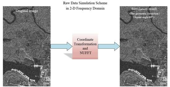
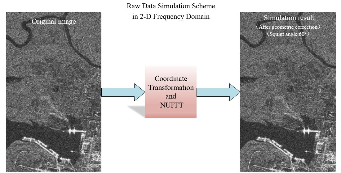
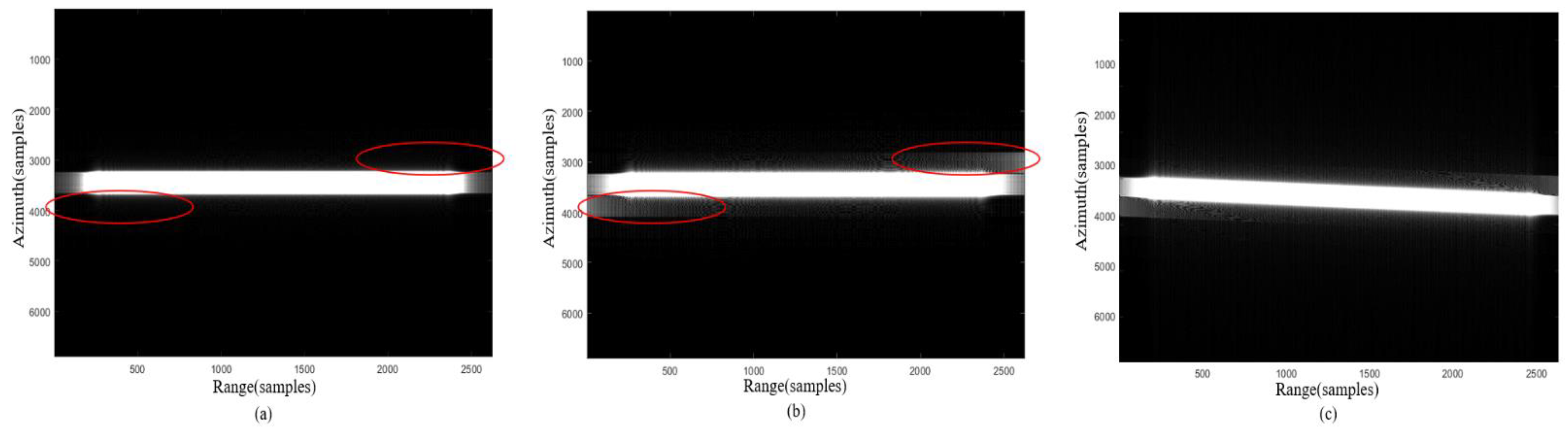
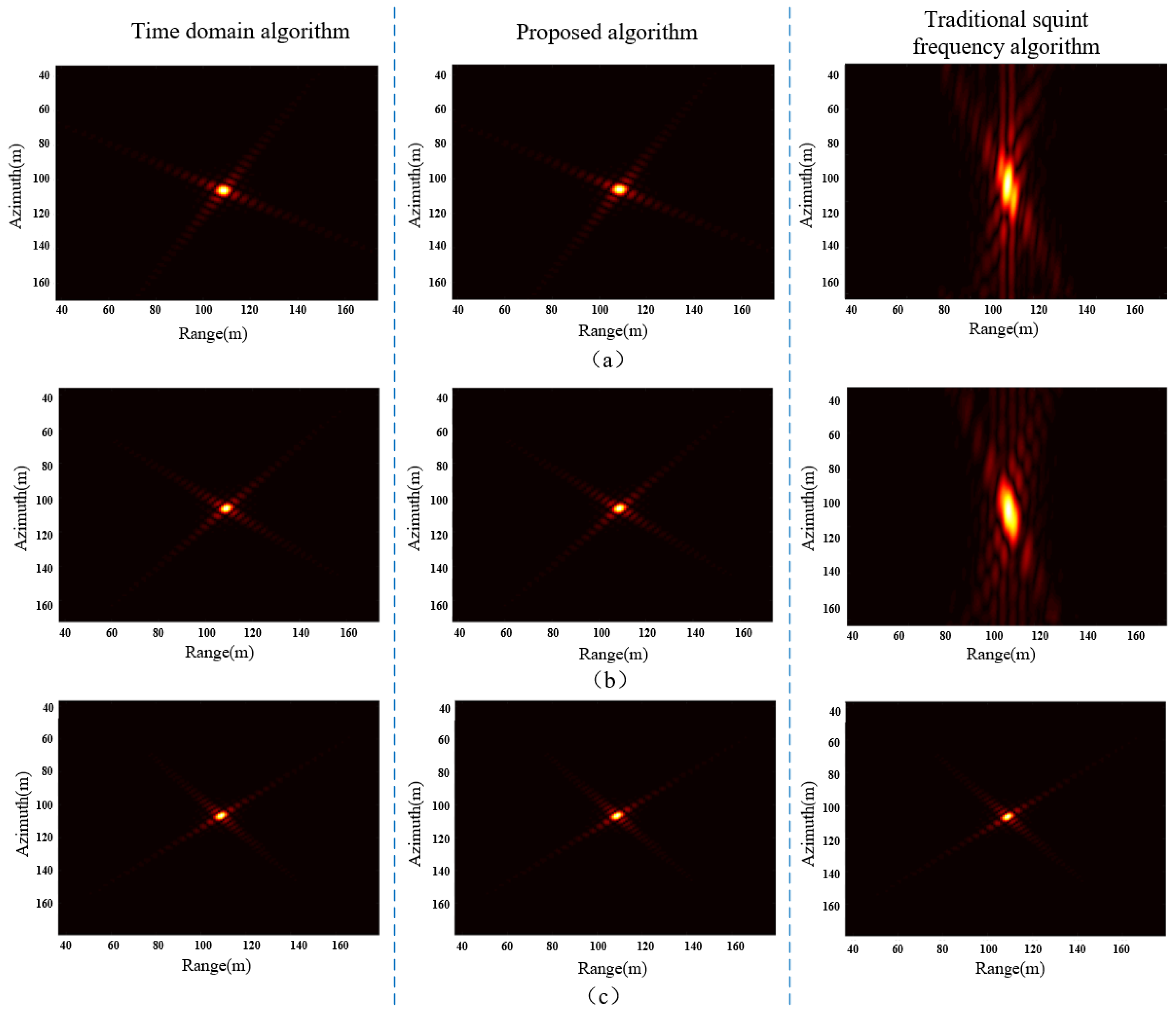
3.1. Simulation Result

The main simulation parameters are shown in

Table 1. Simulation parameters of the point target.

Parameter	Value
Signal pulse width	30 us
Pulse repetition frequency	1500 Hz
Signal bandwidth	50 MHz
Height	10 km
Velocity	200 m/s
Squint angle	30°/45°/60°
Slant range of image center	60 km
Center frequency	9.65 GHz

.

In this experiment, a point target is arranged in the scene. Figure 5a,b shows the 2-D frequency spectrums before and after coordinate transformation, and Figure 5c shows the final 2-D frequency spectrum after compensation of the range walk. It is evident that the space-variant feature, which is observed in the red circles, is well simulated after NUFFT is applied. The simulated imaging results are shown in Figure 6. The point target is well focused in the case of a high squint.

It is widely known that the time domain algorithm has the highest precision, but it has a large computational complexity. Therefore, evaluating the performance of frequency domain algorithms is usually compared with the time domain algorithm. Three different raw data simulation algorithms are used in the same conditions, and different simulation results are imaged via a back-projection algorithm in Figure 6. The peak side lobe ratio (PSLR) and the integrated side lobe ratio (ISLR) are investigated to evaluate the focus quality, and the results are summarized in

Table 2. Comparison of evaluation results for simulated point target.

Squint Angle	Algorithms	PSLR (dB) Azimuth/Range	ISLR (dB) Azimuth/Range
30°	Time domain algorithm	−13.27/−13.26	−11.34/−11.39
	Traditional squint algorithm	−12.81/−12.63	−11.08/−11.13
	Proposed algorithm	−13.16/−13.21	−11.32/−11.28
45°	Time domain algorithm	−13.23/−13.29	−11.70/−11.28
	Traditional squint algorithm	−10.34/−10.89	−10.59/−10.38
	Proposed algorithm	−13.07/−13.13	−11.46/−11.16
60°	Time domain algorithm	−13.25/−13.21	−11.59/−11.32
	Traditional squint algorithm	−7.62/−6.82	−5.89/−6.38
	Proposed algorithm	−12.89/−12.93	−11.02/−10.87

. In addition, the simulation times of different algorithms are shown in

Table 3. Simulation time comparisons.

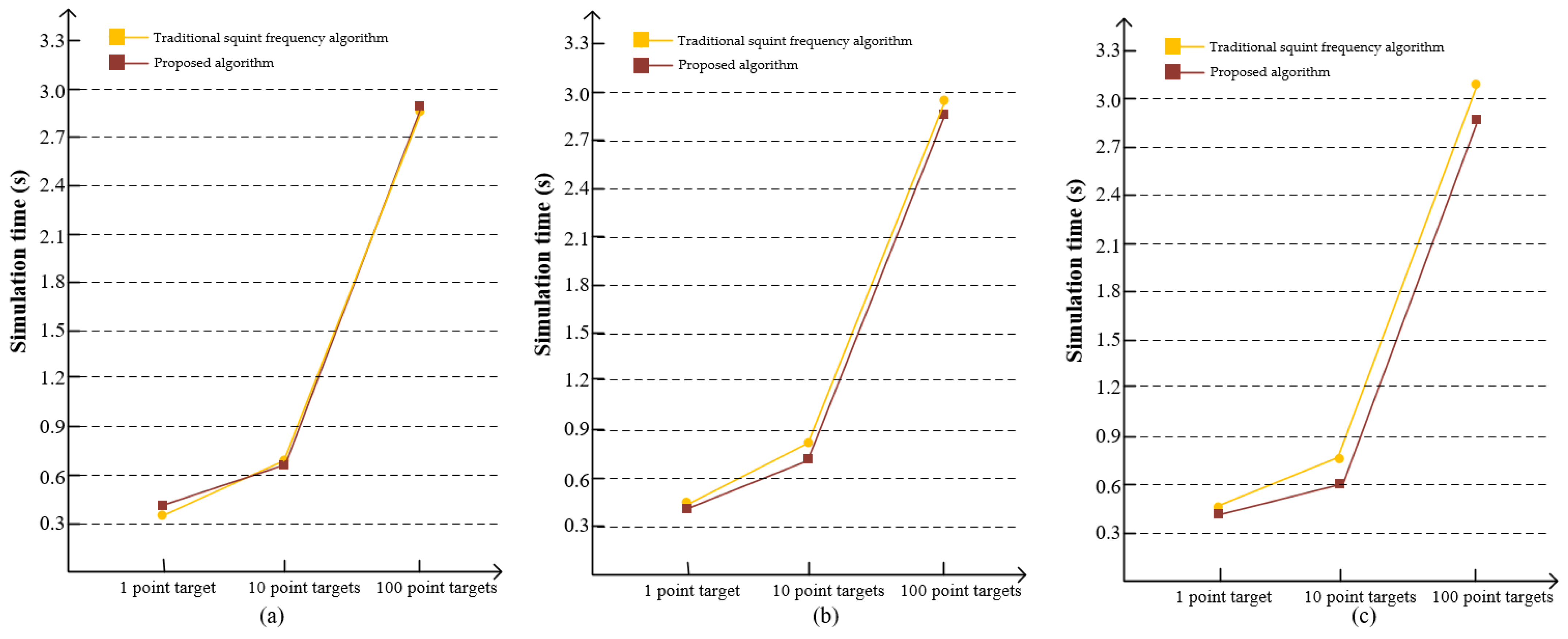
Squint Angle	Algorithms	Simulation Times (s)
		1 Target	10 Targets	100 Targets
30°	Time domain algorithm	3.27	33.55	329.68
	Traditional squint frequency algorithm	0.37	0.69	2.87
	Proposed algorithm	0.41	0.66	2.91
45°	Time domain algorithm	3.67	35.75	332.13
	Traditional squint frequency algorithm	0.43	0.77	2.93
	Proposed algorithm	0.39	0.68	2.88
60°	Time domain algorithm	3.87	37.53	339.53
	Traditional squint frequency algorithm	0.45	0.73	3.05
	Proposed algorithm	0.42	0.61	2.91

.

As can be seen from Figure 6, Table 2 and Table 3, for a the perspective of simulation quality, the time domain algorithm is not affected by the squint angle and always has high precision. The point target of the traditional squint frequency domain algorithm is well focused under a squint angle of 30°, but the values of PSLR and ISLR are slightly higher than those of the time domain algorithm. Under squint angles of 45° and 60°, the imaging results of the traditional squint frequency domain algorithm are poor, and the values of PSLR and ISLR are significantly higher than those of the time domain algorithm and the proposed algorithm. Therefore, the traditional frequency domain algorithm is not suitable for simulations in cases of high squint. However, the quality of the proposed algorithm is high whatever the squint angle is 30°, 45°, or 60°. Although the proposed algorithm is not as accurate as the time domain algorithm, its imaging result of the point target is well focused. The values of PSLR and ISLR are almost the same as those of the time domain algorithm. In particular, when the squint angle increases, the PSLR and ISLR increase slightly.

From the perspective of simulation efficiency, obviously, the computational efficiency of the frequency domain algorithm is higher than that of the time domain algorithm. The time domain algorithm calculates the raw data of each target in a scene, and this is the reason why the time domain algorithm has a high accuracy and low efficiency. The traditional squint frequency domain algorithm has almost an equivalent efficiency to the proposed algorithm; however, with the increase in squint angle, the computing time of the proposed algorithm is shorter than the computing time of the traditional squint frequency domain algorithm, because the NUFFT of the proposed algorithm saves more time than the interpolation operation of the traditional frequency domain algorithm when the squint angle increases. The computational complexity will be analyzed in Section 3.2.

The phase error of the proposed algorithm compared to the time domain algorithm increases as the squint angle increases, and the phase error is at its maximum under a squint of 60°. However, the phase errors of the azimuth and the range are less than 20°, the phase errors are shown in Figure 7, the imaging result will not be affected. Therefore, the accuracy of proposed algorithm is high.

The input image and imaging results of the distributed target simulation after geometric correction are shown in Figure 8, and the simulation parameters of the distributed target are shown in

Table 4. Simulation parameters of the distributed target.

Parameter	Value
Signal pulse width	30 us
Pulse repetition frequency	1300 Hz
Signal bandwidth	60 MHz
Height	5 km
Velocity	400 m/s
Squint angle	60°
Slant range of image center	60 km
Center frequency	9.65 GHz

. From the results of the point target and the distributed target, the proposed algorithm can simulate the original image better than the traditional frequency domain simulation algorithm, and the imaging results of the proposed method are almost the same as those of the input image. More importantly, the proposed algorithm only takes 21 s to complete a distributed target simulation. Compared with the time domain algorithm, the computational efficiency is improved by an order of magnitude.

3.2. Performance Analysis

As noted in the previous description, the entire proposed algorithm primarily includes complex multiplication and additions. The computational complexity is expressed through complex multiplication. Assuming that the size of the raw data is $N_a\times N_r$, $N_a$ is the number of azimuth samples and $N_r$ is the number of range samples. For simplicity, the scene size is also set to $N_a\times N_r$. According to Equation (2), the computational complexity of the time domain algorithm can be expressed as:

$$N_1\approx {\left(N_a·N_r\right)}^2$$

(30)

According to Figure 2, compared with the broadside frequency domain algorithm, the traditional squint frequency domain algorithm requires interpolation operations. Assuming that the computational complexity of interpolation is $N_i$, the computational complexity of traditional squint frequency domain algorithm can be expressed as:

$$N_2\approx N_i+3N_a·N_r+2N_a·N_r{\log }_2{N}_a+2N_a·N_r{\log }_2{N}_r$$

(31)

According to Section 2, assuming that the computational complexity of NUFFT is $N_n$, the computational complexity of the proposed algorithm is expressed as:

$$N_3\approx N_n+3N_a·N_r+2N_a·N_r{\log }_2{N}_a+N_a·N_r{\log }_2{N}_r$$

(32)

It can be seen from Equations (30)–(32) that the proposed algorithm has the lowest complexity, followed by the traditional frequency domain algorithm; the time domain algorithm is the most complicated. Therefore, if raw data simulation seeks a high accuracy and there is no limitation to efficiency, the time domain algorithm should be selected. However, if a mission needs to simulate an image quickly and accurately in the case of high squint, the proposed algorithm is undoubtedly the best choice.

4. Discussion

From the above experiment results, we discuss the proposed method from the following three aspects: hardware requirement, accuracy, and efficiency.

First, the proposed algorithm can quickly simulate raw data without high-performance hardware. The simulation platform and hardware information are listed in

Table 5. Simulation platform and hardware information.

Platform	Information
CPU	Inter Xeon Gold 6126
	Number of Core: 48
	Clock Speed: 2.6 GHz
Memory	128 GB
Computing software	MATLAB 9.4 (R2018a)
Operating system	Windows 10

. It can be seen that the hardware requirements of the proposed algorithm are not strict. However, other time domain acceleration algorithms proposed by some researchers require a high-performance central processing unit (CPU) and graphics processing unit (GPU), for example, the algorithms in [17,18,19,20,21] require a powerful CPU and GPU for acceleration.

Second, in this paper, a back-projection algorithm is used to image the generated raw data. A back-projection algorithm is an accurate imaging algorithm, which is not affected by any factors. This imaging algorithm can accurately correspond to the information of raw data; therefore, in order to evaluate the accuracy of the generated raw data, the back-projection algorithm is used. We take the results from the BP algorithm as an evaluation standard to determine the accuracy of the raw data simulation. The accuracy of existing frequency domain raw data simulation algorithms is not satisfactory, especially in the case of high squint. The proposed algorithm is different from the traditional frequency domain simulation algorithm; we considered another approach, using the method of coordinate transformation. On the one hand, the proposed algorithm retains the high efficiency of the traditional frequency domain raw data simulation algorithm. On the other hand, through coordinate transformation and NUFFT, the accuracy is higher than that of the traditional frequency domain raw data simulation algorithm in the case of high squint.

Finally, in terms of efficiency, the traditional time domain algorithm has a very large amount of needed computation, and it calculates the raw data of each point in turn. However, the proposed algorithm in this paper adopts a unified processing method for all points through a transfer function in the frequency domain, and this computing mode is efficient. In addition, the computational complexity is shown in Section 3.2, and, compared with the time domain algorithm, the proposed algorithm has great advantages in terms of the amount of computation. In order to clearly show the operation time of the traditional squint frequency algorithm and the proposed algorithm, we created line charts, as shown in Figure 9, according to Table 3, and these line charts can more clearly show the changes in the trends of the computational efficiency. Due to the computational time of the time domain algorithm being much higher than that of the frequency domain algorithm, we do not show the time of the time domain algorithm on the line chart. As can be seen from Figure 9, the traditional squint frequency domain algorithm has almost the same efficiency as the proposed algorithm. With an increase in squint angle, the computing time of the proposed algorithm is shorter than that of the computing time of the traditional squint frequency domain algorithm. The proposed algorithm is more suitable for raw data simulation than the traditional squint frequency domain algorithm in the case of large squint.

In future work, we will continue to focus on how to improve the accuracy of the proposed algorithm and maintain the original computational efficiency. By referring to the imaging algorithm, we will continue to seek an algorithm that can improve the accuracy of raw data simulations. In addition, the recent deep automated image quality analysis method is also a potential direction.

5. Conclusions

High-squint SAR suffers from the range-azimuth coupling effect, and it is the reason why the frequency domain simulation algorithm is invalid when a squint angle exists. We analyzed the geometries of broadside and high-squint spotlight SAR. According to the different geometries, a frequency domain simulation algorithm based on coordinate transformation and NUFFT is proposed. NUFFT is used to solve problems after coordinate transformations. Comparative experiments show that the proposed algorithm simulates the characteristics of high-squint SAR, as well as point and distributed target imaging results and is well focused under a high squint angle. More importantly, the accuracy of the proposed algorithm is higher than that of the traditional algorithm. In addition, the computational efficiency of the proposed algorithm can be significantly improved, in contrast to the traditional time domain algorithm. In the future, relevant research will continue. We will focus on methods to reduce any artifacts in high-squint spotlight SAR simulated data generation; for example, recent deep automated image quality analysis methods [38] of the proposed algorithm show great potential, in the simulation of high-squint spotlight SAR raw data simulations.

References

- Li, D.; Rodriguez-Cassola, M.; Prats-Iraola, P.; Wu, M.; Moreira, A. Reverse Backprojection Algorithm for the Accurate Generation of SAR Raw Data of Natural Scenes. IEEE Geosci. Remote Sens. Lett. 2017, 14, 2072–2076. [Google Scholar] [CrossRef] [Green Version]
- Zhang, Y.; Sun, J.; Lei, P.; Hong, W. SAR-Based Paired Echo Focusing and Suppression of Vibrating Targets. IEEE Trans. Geosci. Remote Sens. 2014, 52, 7593–7605. [Google Scholar] [CrossRef]
- Niu, S.; Qiu, X.; Lei, B.; Ding, C.; Fu, K. Parameter Extraction Based on Deep Neural Network for SAR Target Simulation. IEEE Trans. Geosci. Remote Sens. 2020, 58, 4901–4914. [Google Scholar] [CrossRef]
- Tong, X.; Bao, M.; Sun, G.; Han, L.; Zhang, Y.; Xing, M. Refocusing of Moving Ships in Squint SAR Images Based on Spectrum Orthogonalization. Remote Sens. 2021, 13, 2807. [Google Scholar] [CrossRef]
- Huai, Y.; Liang, Y.; Ding, J.; Xing, M.; Zeng, L.; Li, Z. An Inverse Extended Omega-K Algorithm for SAR Raw Data Simulation With Trajectory Deviations. IEEE Geosci. Remote Sens. Lett. 2016, 13, 826–830. [Google Scholar] [CrossRef]
- Li, N.; Zhang, H.; Zhao, J.; Wu, L.; Guo, Z. An Azimuth Signal-Reconstruction Method Based on Two-Step Projection Technology for Spaceborne Azimuth Multi-Channel High-Resolution and Wide-Swath SAR. Remote Sens. 2021, 13, 4988. [Google Scholar] [CrossRef]
- Li, N.; Shen, Q.; Wang, L.; Wang, Q.; Guo, Z.; Zhao, J. Optimal time selection for ISAR imaging of ship targets based on time-frequency analysis of multiple scatterers. IEEE Geosci. Remote Sens. Lett. 2021, 19, 1–5. [Google Scholar] [CrossRef]
- Xing, M.; Wu, Y.; Zhang, Y.; Sun, G.; Bao, Z. Azimuth Resampling Processing for Highly Squinted Synthetic Aperture Radar Imaging with Several Modes. IEEE Trans. Geosci. Remote Sens. 2014, 52, 4339–4352. [Google Scholar] [CrossRef]
- Fan, W.; Zhang, M.; Li, J.; Wei, P. Modified Range-Doppler Algorithm for High Squint SAR Echo Processing. IEEE Geosci. Remote Sens. Lett. 2019, 16, 422–426. [Google Scholar] [CrossRef]
- Chiang, C.-Y.; Chen, K.-S.; Yang, Y.; Zhang, Y.; Zhang, T. SAR Image Simulation of Complex Target including Multiple Scattering. Remote Sens. 2021, 13, 4854. [Google Scholar] [CrossRef]
- Jiang, W.; Wang, Y.; Li, Z.; Liu, G.; Zhang, M. Simulation of a Wideband Radar Echo of a Target on a Dynamic Sea Surface. Remote Sens. 2021, 13, 3186. [Google Scholar] [CrossRef]
- Ku, C.; Chen, K.; Chang, P.; Chang, Y. Imaging Simulation for Synthetic Aperture Radar: A Full-Wave Approach. Remote Sens. 2018, 10, 1404. [Google Scholar] [CrossRef] [Green Version]
- Xiao, P.; Liu, M.; Guo, W.; Chen, W. Reconstruction of Synthetic Aperture Radar Raw Data under Analog-To-Digital Converter Saturation Distortion for Large Dynamic Range Scenes. Remote Sens. 2019, 11, 1043. [Google Scholar] [CrossRef] [Green Version]
- Qian, Y.; Zhu, D. Image Formation of Azimuth Periodically Gapped SAR Raw Data with Complex Deconvolution. Remote Sens. 2019, 11, 2698. [Google Scholar] [CrossRef] [Green Version]
- Ma, B.; Yu, B.; Liu, C.; Wang, Y. A 2-D Fourier Domain Algorithm for StripMap FMCW-SAR Raw Signal Simulation. J. Electron. Inf. Technol. 2011, 33, 375–380. [Google Scholar] [CrossRef]
- Wei, L.; Li, S.; Wu, Y.; Xiang, M. Performance Comparison of Algorithms for SAR Raw Signal Generation. J. Electron. Inf. Technol. 2005, 27, 262–265. [Google Scholar]
- Fu, Z.; Bai, L.; Guo, Z.; Min, L.; Li, N. Research on Acceleration Algorithm for Raw Data Simulation of High Resolution Squint Spotlight SAR. In Proceedings of the 2021 IEEE International Geoscience and Remote Sensing Symposium (IGARSS 2021), Brussels, Belgium, 11–16 July 2021; pp. 3281–3284. [Google Scholar] [CrossRef]
- Zhang, F.; Hu, C.; Li, W.; Hu, W.; Wang, P.; Li, H. A Deep Collaborative Computing Based SAR Raw Data Simulation on Multiple CPU/GPU Platform. IEEE J. Sel. Top. Appl. Earth Obs. Remote Sens. 2017, 10, 387–399. [Google Scholar] [CrossRef]
- Zhang, F.; Yao, X.; Tang, H.; Yin, Q.; Hu, Y.; Lei, B. Multiple Mode SAR Raw Data Simulation and Parallel Acceleration for Gaofen-3 Mission. IEEE J. Sel. Top. Appl. Earth Obs. Remote Sens. 2018, 11, 2115–2126. [Google Scholar] [CrossRef]
- Zhang, F.; Hu, C.; Li, W.; Hu, W.; Wang, P. Accelerating Time-Domain SAR Raw Data Simulation for Large Areas Using Multi-GPUs. IEEE J. Sel. Top. Appl. Earth Obs. Remote Sens. 2014, 7, 3956–3966. [Google Scholar] [CrossRef]
- Jing, G.; Zhang, Y.; Li, Z.; Sun, G.; Xing, M.; Bao, Z. Efficient Realiazation of SAR Echo Simulation Based on GPU. J. Syst. Eng. Electron. 2016, 38, 2493–2498. [Google Scholar] [CrossRef]
- Franceschetti, G.; Schirinzi, G. A SAR Processor Based on Two Dimensional FFT Codes. IEEE Trans. Aerosp. Electron. Syst. 1990, 26, 356–366. [Google Scholar] [CrossRef]
- Franceschetti, G.; Migliaccio, M.; Riccio, D.; Schirinzi, G. SARAS: A Synthetic Aperture Radar (SAR) Raw Signal Simulator. IEEE Trans. Geosci. Remote Sens. 1992, 30, 110–123. [Google Scholar] [CrossRef]
- Franceschetti, G.; Migliaccio, M.; Riccio, D. On ocean SAR raw signal simulation. IEEE Trans. Geosci. Remote Sens. 1998, 36, 84–100. [Google Scholar] [CrossRef]
- Franceschetti, G.; Lanari, R.; Marzouk, E. A New Two-Dimensional Squint Mode SAR Processor. IEEE Trans. Aerosp. Electron. Syst. 1996, 32, 854–863. [Google Scholar] [CrossRef]
- Franceschetti, G.; Lodice, A.; Riccio, D.; Ruello, G.; Siviero, R. SAR Raw Signal Simulation of Oil Slicks in Ocean Environments. IEEE Trans. Geosci. Remote Sens. 2002, 40, 1935–1949. [Google Scholar] [CrossRef]
- Franceschetti, G.; Lodice, A.; Riccio, D.; Ruello, G. SAR Raw Singal Simulation for Urban Structures. IEEE Trans. Geosci. Remote Sens. 2003, 41, 1986–1995. [Google Scholar] [CrossRef]
- Franceschetti, G.; Lodice, A.; Perna, S.; Riccio, D. Efficient Simulation of Airborne SAR Raw Data of Extended Scenes. IEEE Trans. Geosci. Remote Sens. 2006, 44, 2851–2860. [Google Scholar] [CrossRef]
- Franceschetti, G.; Guida, R.; Lodice, A.; Riccio, D.; Ruello, G. Efficient Simulation of Hybrid Stripmap/Spotlight SAR Raw Signals from Extended Scenes. IEEE Trans. Geosci. Remote Sens. 2006, 42, 2385–2396. [Google Scholar] [CrossRef]
- Franceschetti, G.; Lodice, A.; Perna, S.; Riccio, D. SAR Sensor Trajectory Deviations: Fourier Domain Formulation and Extended Scene Simulation of Raw Signal. IEEE Trans. Geosci. Remote Sens. 2006, 44, 2323–2334. [Google Scholar] [CrossRef]
- Wang, Y.; Zhang, Z.; Deng, Y. Squint Spotlight SAR Raw Signal Simulation in the Frequency Domain Using Optical Principles. IEEE Trans. Geosci. Remote Sens. 2008, 46, 2208–2215. [Google Scholar] [CrossRef]
- Diao, G.; Xu, X. Fast Algorithm for SAR Raw Data Simulation with Large Squint Angles. J. Electron. Inf. Technol. 2011, 33, 684–689. [Google Scholar] [CrossRef]
- Li, G.; Ma, Y.; Hou, J.; Xu, G. Sub-aperture Keystone Transform Based Echo Simulation Method for High-squint SAR with a Curve Trajectory. J. Electron. Inf. Technol. 2020, 42, 2261–2268. [Google Scholar] [CrossRef]
- Breglia, A.; Capozzoli, A.; Curcio, C.; Liseno, A. NUFFT-Based Interpolation in Backprojection Algorithms. IEEE Geosci. Remote Sens. Lett. 2021, 18, 2117–2121. [Google Scholar] [CrossRef]
- Hu, R.; Li, X.; Yeo, T.; Yang, Y.; Chi, C.; Zuo, F.; Hu, X.; Pi, Y. Refocusing and Zoom-In Polar Format Algorithm for Curvilinear Spotlight SAR Imaging on Arbitrary Region of Interest. IEEE Trans. Geosci. Remote Sens. 2019, 57, 7995–8010. [Google Scholar] [CrossRef]
- Zhao, S.; Deng, Y.; Wang, R. Imaging for High-Resolution Wide-Swath Spaceborne SAR Using Cubic Filtering and NUFFT Based on Circular Orbit Approximation. IEEE Trans. Geosci. Remote Sens. 2016, 55, 787–800. [Google Scholar] [CrossRef]
- Capozzoli, A.; Curio, C.; Liseno, A. Optimized Nonuniform FFTs and Their Application to Array Factor Computation. IEEE T Antenn Propag. 2019, 67, 3924–3938. [Google Scholar] [CrossRef]
- Mukherjee, S.; Valenzise, G.; Cheng, I. Potential of Deep Features for Opinion-Unaware, Distortion-Unaware, No-Reference Image Quality. Lect. Notes Comput. Sci. 2020, 2015, 87–95. [Google Scholar] [CrossRef]