
LiDAR-Visual-Inertial Odometry Based on Optimized Visual Point-Line Features

Abstract
:
1. Introduction
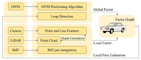
2. System Overview
3. Front-End: Feature Extraction and Matching Tracking
3.1. Line Feature Extraction
3.2. Inter-Frame Feature Constraint Matching
3.3. LiDAR-Aided Depth Correlation of Visual Features
4. Back-End: LVIO-GNSS Fusion Framework Based on Factor Graph
4.1. Construction of Factor Graph Optimization Framework
4.2. IMU Factor
4.3. Visual Feature Factor
4.3.1. Visual Point Feature Factor
4.3.2. Visual Line Feature Factor
4.4. LiDAR Factor
4.5. GNSS Factor and Loop Factor
5. Experimental Results
5.1. Real-Time Performance
5.1.1. Indoor Environment
5.1.2. Outdoor Environment
5.2. Positioning Accuracy
5.2.1. Indoor Environment
5.2.2. Outdoor Environment
5.3. Mapping Performance
6. Discussion
7. Conclusions
Author Contributions
Funding
Institutional Review Board Statement
Informed Consent Statement
Data Availability Statement
Conflicts of Interest
References
- Qian, Q.; Bai, T.M.; Bi, Y.F.; Qiao, C.Y.; Xiang, Z.Y. Monocular Simultaneous Localization and Mapping Initialization Method Based on Point and Line Features. Acta Opt. Sin. 2021, 41, 1215002. [Google Scholar]
- Shan, T.; Englot, B. LeGO-LOAM: Lightweight and Ground-Optimized Lidar Odometry and Mapping on Variable Terrain. In Proceedings of the 2018 IEEE/RSJ International Conference on Intelligent Robots and Systems (IROS), Madrid, Spain, 1–5 October 2018; pp. 4758–4765. [Google Scholar]
- Zuo, X.; Xie, X.; Liu, Y.; Huang, G. Robust visual SLAM with point and line features. In Proceedings of the 2017 IEEE/RSJ International Conference on Intelligent Robots and Systems (IROS), Vancouver, BC, Canada, 24–28 September 2017; pp. 1775–1782. [Google Scholar]
- Zhang, J.; Singh, S. Laser-Visual-Inertial Odometry and Mapping with High Robustness and Low Drift. J. Field Robot. 2018, 35, 1242–1264. [Google Scholar] [CrossRef]
- Qin, T.; Li, P.; Shen, S. Vins-mono: A robust and versatile monocular visual-inertial state estimator. IEEE Trans. Robot. 2018, 34, 1004–1020. [Google Scholar] [CrossRef] [Green Version]
- Mur-Artal, R.; Tardós, J.D. ORB-SLAM2: An open-source slam system for monocular, stereo, and rgb-d cameras. IEEE Trans. Robot. 2018, 33, 1255–1262. [Google Scholar] [CrossRef] [Green Version]
- Forster, C.; Carlone, L.; Dellaert, F.; Scaramuzza, D. On-manifold preintegration for real-time visual–inertial odometry. IEEE Trans. Robot. 2017, 33, 1–21. [Google Scholar] [CrossRef] [Green Version]
- Forster, C.; Zhang, Z.; Gassner, M.; Werlberger, M.; Scaramuzza, D. SVO: Semi-direct visual odometry for monocular and multicamera systems. IEEE Trans. Robot. 2016, 33, 249–265. [Google Scholar] [CrossRef] [Green Version]
- He, Y.; Zhao, J.; Guo, Y.; He, W.H.; Yuan, K. Pl-vio: Tightly-coupled monocular visual–inertial odometry using point and line features. Sensors 2018, 18, 1159. [Google Scholar] [CrossRef] [PubMed] [Green Version]
- Wen, H.; Tian, J.; Li, D. PLS-VIO: Stereo Vision-inertial Odometry Based on Point and Line Features. In Proceedings of the 2020 International Conference on High Performance Big Data and Intelligent Systems (HPBD&IS), Shenzhen, China, 23 May 2020. [Google Scholar]
- Pumarola, A.; Vakhitov, A.; Agudo, A.; Sanfeliu, A.; Moreno-Noguer, F. PL-SLAM: Real-time monocular visual SLAM with points and lines. In Proceedings of the 2017 IEEE International Conference on Robotics and Automation (ICRA), Singapore, 29 May–3 June 2017; pp. 4503–4508. [Google Scholar]
- Fu, Q.; Wang, J.; Yu, H.; Ali, I.; Zhang, H. PL-VINS: Real-Time Monocular Visual-Inertial SLAM with Point and Line. [DB/OL]. Available online: https://arxiv.org/abs/2009.07462v1 (accessed on 27 November 2021).
- Zhang, J.; Singh, S. LOAM: Lidar Odometry and Mapping in Real-time. In Proceedings of the 2014 Robotics: Science and Systems, Berkeley, CA, USA, 12–16 July 2014; pp. 9–17. [Google Scholar]
- Shan, T.; Englot, B.; Meyers, D.; Wang, W.; Rus, D. LIO-SAM: Tightly-Coupled Lidar Inertial Odometry via Smoothing and Mapping. [DB/OL]. Available online: https://arxiv.org/abs/2007.00258v3 (accessed on 27 November 2021).
- Xiang, Z.; Yu, J.; Li, J.; Su, J. ViLiVO: Virtual LiDAR-Visual Odometry for an Autonomous Vehicle with a Multi-Camera System. In Proceedings of the 2019 IEEE/RSJ International Conference on Intelligent Robots and Systems (IROS), Macao, China, 3–8 November 2019; pp. 2486–2492. [Google Scholar]
- Chen, S.; Zhou, B.; Jiang, C.; Xue, W.; Li, Q. A LiDAR/Visual SLAM Backend with Loop Closure Detection and Graph Optimization. Remote Sens. 2021, 13, 2720. [Google Scholar] [CrossRef]
- Lin, J.; Zheng, C.; Xu, W.; Zhang, F. R2LIVE: A Robust, Real-Time, LiDAR-Inertial-Visual Tightly-Coupled State Estimator and Mapping. [DB/OL]. Available online: https://arxiv.org/abs/2102.12400 (accessed on 27 November 2021).
- Huang, S.; Ma, Z.; Mu, T.; Fu, H.; Hu, S. Lidar-Monocular Visual Odometry using Point and Line Features. In Proceedings of the 2020 IEEE International Conference on Robotics and Automation(ICRA), Online, 1–15 June 2020; pp. 1091–1097. [Google Scholar]
- Zhou, L.; Wang, S.; Kaess, M. DPLVO: Direct Point-Line Monocular Visual Odometry. IEEE Robot. Autom. Lett. 2021, 6, 7113–7120. [Google Scholar] [CrossRef]
- He, X.; Pan, S.G.; Tan, Y.; Gao, W.; Zhang, H. VIO-GNSS Location Algorithm Based on Point-Line Feature in Outdoor Scene. Laser Optoelectron. Prog. 2022, 56, 1815002. [Google Scholar]
- Silva, V.D.; Roche, J.; Kondoz, A. Fusion of LiDAR and camera sensor data for environment sensing in driverless vehicles. arXiv 2018, arXiv:1710.06230. [Google Scholar]
- Liu, X.; Li, D.; Shi, J.; Li, A.; Jiang, L. A framework for low-cost Fusion Positioning with Single Frequency RTK/MEMS-IMU/VIO. J. Phys. Conf. Ser. 2021, 1738, 012007. [Google Scholar] [CrossRef]
- Mascaro, R.; Teixeira, L.; Hinzmann, T.; Siegwart, R.; Gomsf, M.C. Graph-optimization based multi-sensor fusion for robust uav pose estimation. In Proceedings of the 2018 IEEE International Conference on Robotics and Automation(ICRA), Brisbane, Australia, 21–24 May 2018; pp. 1421–1428. [Google Scholar]
- Woosik, L.; Eckenhoff, K.; Geneva, P.; Huang, G.Q. Intermittent GPS-aided VIO: Online Initialization and Calibration. In Proceedings of the 2018 IEEE International Conference on Robotics and Automation(ICRA), Paris, France, 31 May–6 June 2020; pp. 5724–5731. [Google Scholar]
- Qin, T.; Cao, S.; Pan, J.; Shen, S. A General Optimization-Based Framework for Global Pose Estimation with Multiple Sensors. [DB/OL]. Available online: https://arxiv.org/abs/1901.03642 (accessed on 27 November 2021).
- Fernandes, L.A.F.; Oliveira, M.M. Real-time line detection through an improved Hough transform voting scheme. Pattern Recognit. 2008, 41, 299–314. [Google Scholar] [CrossRef]
- Nieto, M.; Cuevas, C.; Salgado, L.; Narciso, G. Line segment detection using weighted mean shift procedures on a 2D slice sampling strategy. Pattern Anal. Appl. 2011, 14, 149–163. [Google Scholar] [CrossRef]
- Akinlar, C.; Topal, C. EDLines: A real-time line segment detector with a false detection control. Pattern Recognit. Lett. 2011, 32, 1633–1642. [Google Scholar] [CrossRef]
- Gioi, R.; Jakubowicz, J.; Morel, J.M.; Randall, G. LSD: A fast line segment detector with a false detection control. IEEE Trans. Pattern Anal. Mach. Intell. 2010, 32, 722–732. [Google Scholar] [CrossRef] [PubMed]
- Shan, T.; Englot, B.; Ratti, C.; Rus, D. LVI-SAM: Tightly-Coupled Lidar-Visual-Inertial Odometry via Smoothing and Mapping. [DB/OL]. Available online: https://arxiv.org/abs/2104.10831 (accessed on 27 November 2021).


| Sequence | Vins_Mono (w/o loop) | Vins_Mono (w/ loop) | PL-VIO | LVI-SAM | Purposed |
|---|---|---|---|---|---|
| ATE_RMSE(m)/Mean Error(m) | |||||
| MH_01_easy | 0.213/0.189 | 0.188/0.158 | 0.093/0.081 | 0.181/0.147 | 0.073/0.062 |
| MH_02_easy | 0.235/0.193 | 0.188/0.157 | 0.072/0.062 | 0.182/0.167 | 0.045/0.039 |
| MH_03_medium | 0.399/0.321 | 0.402/0.315 | 0.260/0.234 | 0.400/0.308 | 0.056/0.050 |
| MH_04_difficult | 0.476/0.423 | 0.422/0.348 | 0.364/0.349 | 0.398/0.399 | 0.079/0.075 |
| MH_05_difficult | 0.426/0.384 | 0.370/0.309 | 0.251/0.238 | 0.380/0.287 | 0.139/0.127 |
| V1_01_easy | 0.157/0.137 | 0.145/0.121 | 0.078/0.067 | 0.142/0.119 | 0.040/0.037 |
| V1_03_difficult | 0.314/0.275 | 0.329/0.289 | 0.205/0.179 | 0.322/0.283 | 0.077/0.069 |
| V2_01_easy | 0.133/0.115 | 0.120/0.108 | 0.086/0.072 | 0.121/0.110 | 0.056/0.048 |
| V2_02_medium | 0.287/0.244 | 0.293/0.255 | 0.150/0.097 | 0.291/0.250 | 0.089/0.078 |
| V2_03_difficult | 0.343/0.299 | 0.351/0.315 | 0.273/0.249 | 0.351/0.308 | 0.098/0.092 |
| Sequence | Hong Kong 0428 | Hong Kong 0314 |
|---|---|---|
| ATE_RMSE(m)/Mean Error(m) | ||
| Vins_Mono (w/o loop) | 101.735/89.470 | 40.651/35.035 |
| Vins_Mono (w/ loop) | 76.179/67.535 | 19.191/15.617 |
| LIO-SAM | 7.181/6.787 | 41.933/39.672 |
| LVI-SAM | 9.764/9.061 | 3.065/2.557 |
| Purposed(*) | 9.475/8.884 | 2.842/2.456 |
| Purposed(#) | 5.808/5.436 | 2.595/2.041 |
| Purposed | 5.299/4.955 | 2.249/1.880 |
Publisher’s Note: MDPI stays neutral with regard to jurisdictional claims in published maps and institutional affiliations. |
© 2022 by the authors. Licensee MDPI, Basel, Switzerland. This article is an open access article distributed under the terms and conditions of the Creative Commons Attribution (CC BY) license (https://creativecommons.org/licenses/by/4.0/).
Share and Cite
He, X.; Gao, W.; Sheng, C.; Zhang, Z.; Pan, S.; Duan, L.; Zhang, H.; Lu, X. LiDAR-Visual-Inertial Odometry Based on Optimized Visual Point-Line Features. Remote Sens. 2022, 14, 622. https://doi.org/10.3390/rs14030622
He X, Gao W, Sheng C, Zhang Z, Pan S, Duan L, Zhang H, Lu X. LiDAR-Visual-Inertial Odometry Based on Optimized Visual Point-Line Features. Remote Sensing. 2022; 14(3):622. https://doi.org/10.3390/rs14030622
Chicago/Turabian StyleHe, Xuan, Wang Gao, Chuanzhen Sheng, Ziteng Zhang, Shuguo Pan, Lijin Duan, Hui Zhang, and Xinyu Lu. 2022. "LiDAR-Visual-Inertial Odometry Based on Optimized Visual Point-Line Features" Remote Sensing 14, no. 3: 622. https://doi.org/10.3390/rs14030622