Article

Combined Use of Aerial Photogrammetry and Terrestrial Laser Scanning for Detecting Geomorphological Changes in Hornsund, Svalbard

by
Małgorzata Błaszczyk
1,*,
Michał Laska
1,
Agnar Sivertsen
2 and
Shridhar D. Jawak
3
1
Institute of Earth Sciences, University of Silesia in Katowice, Bedzinska 60, 41-200 Sosnowiec, Poland
2
NORCE Norwegian Research Center AS, Sykehusvn 21, 9019 Tromsø, Norway
3
Svalbard Integrated Arctic Earth Observing System (SIOS), SIOS Knowledge Centre, Svalbard Science Centre, P.O. Box 156, N-9171 Longyearbyen, Norway
*
Author to whom correspondence should be addressed.
Remote Sens. 2022, 14(3), 601; https://doi.org/10.3390/rs14030601
Submission received: 23 December 2021 / Revised: 19 January 2022 / Accepted: 25 January 2022 / Published: 26 January 2022

Abstract

:
The Arctic is a region undergoing continuous and significant changes in land relief due to different glaciological, geomorphological and hydrogeological processes. To study those phenomena, digital elevation models (DEMs) and highly accurate maps with high spatial resolution are of prime importance. In this work, we assess the accuracy of high-resolution photogrammetric DEMs and orthomosaics derived from aerial images captured in 2020 over Hornsund, Svalbard. Further, we demonstrate the accuracy of DEMs generated using point clouds acquired in 2021 with a Riegl VZ®-6000 terrestrial laser scanner (TLS). Aerial and terrestrial data were georeferenced and registered based on very reliable ground control points measured in the field. Both DEMs, however, had some data gaps due to insufficient overlaps in aerial images and limited sensing range of the TLS. Therefore, we compared and integrated the two techniques to create a continuous and gapless DEM for the scientific community in Svalbard. This approach also made it possible to identify geomorphological activity over a one-year period, such as the melting of ice cores at the periglacial zone, changes along the shoreline or snow thickness in gullies. The study highlights the potential for combining other techniques to represent the active processes in this region.

Graphical Abstract

1. Introduction

The Hornsund area in southern Spitsbergen (Svalbard) is the focus of wide glaciological [1,2,3,4], hydrological [5,6,7,8,9], snow [9], permafrost [10,11], geomorphometric [12,13,14] and biological [15] studies performed due to intensive alterations in the surveyed terrain. Digital mapping of such an environment and its related phenomena has become a fundamental requirement to keep track of all such alterations [16]. The most up-to-date, accurate and precise digital elevation models (DEM) for the study area are generated based on high-resolution satellites and aerial photos [17]. From these, the DEM with the highest spatial resolution (2 m) and accuracy (standard deviation = 0.6 m) is derived from aerial photographs taken in 2011. However, to monitor climate-induced change in the territory, there is a need for more frequent and accurate data on terrain elevation [17].
The aim of the paper is to examine and combine two DEMs produced from aerial image sets and terrestrial laser scanning (TLS). All data created within the project are further available to the scientific community through the Svalbard Integrated Arctic Earth Observing System (SIOS). Aerial images for the studied area were provided by SIOS through a dedicated call of proposals (https://sios-svalbard.org/AirborneRS (accessed on 23 December 2021)). One of SIOS’s missions is to reduce the environmental footprint of scientific observations in Svalbard [18]. To achieve this mission, SIOS supports and coordinates the usage of unmanned aerial vehicles (UAVs) and a crewed Dornier aircraft to acquire imagery and hyperspectral data for the Svalbard research community to support scientific projects (https://sios-svalbard.org/AirborneRemoteSensing (accessed on 23 December 2021)). The project started in 2020 and so far, no publications have presented the accuracy of the data collected within the framework of the project. In this study, we examine and present the accuracy of products such as orthomosaics and DEMs obtained during the mission. The aerial data over two Hornsund zones, the Fuglebergsletta and Werenskioldbreen areas, were collected in June 2020 (Figure 1). The mission took place at the beginning of the ablation season, when some snow cover was present in the numerous gullies. Additionally, the flight level limited the sidelap of images, causing data gaps in the DEM. To address these limitations, a long-range TLS campaign was performed in August 2021. Long-range terrestrial laser scanning is an emerging method for the monitoring of complex and rough terrain such as mountain slopes, outcrops and deformations [16,19,20,21,22,23]. Here, we used the ultra-long laser scanner Riegl VZ®-6000, which has been successfully used in cryosphere studies such as glacier mass balance measurements in China [24,25]; the mass balance of very small glaciers in the Swiss Alps [26]; snow distribution at a glacier located in the Ötztal Alps, Austria [27]; glacier snowline determination [28]; or relationships between different climate forcing and flows of Helheim Glacier, Greenland [29]. However, at this point there are not many studies on the accuracy of ultra-long laser scans [23,26,30], especially over 2 km [27]. Further, to our knowledge there has not yet been a study published concerning the quality control of TLS-collected data with the Riegl VZ®-6000 instrument in the polar region. To fill this gap, we analyzed the accuracy of the relative and absolute registration of four scans collected over the complex Fuglebergsletta area, the most studied area near the Polish Polar Station.
Terrestrial laser scanning (TLS) was next applied to complement the aerial photogrammetry. The integration of 3D modeling techniques is advantageous for obtaining the most complete and useful object coverage for many application areas [19]. Integration of aircraft-based, helicopter-based and UAV photogrammetry with TLS is popular, especially at large or inaccessible sites [21,23,30,31,32]. In this paper, digital aerial photogrammetry and TLS were combined to produce a continuous DEM with the highest possible resolution and accuracy. Thanks to that, this DEM, based on aerial photos and scanning (TLS), can be successfully applied to many environmental applications, such as hydrology modeling, glacier change detection, quantifying depositional and erosional processes in dynamic and complex fluvial systems, the evolution of the landscape, geomorphology and the monitoring of landslide displacement [13,33].

2. Study Area

The study area is located in the southern part of Spitsbergen, Svalbard (Figure 1). The area is characterized by diverse surface coverage such as relatively flat topography, mountains, tidewater glaciers and land-based glaciers. Narrow coastal plains with raised marine terraces surround the fjord shores [34]. Further inland, mountain massifs range in elevation up to 763 m above sea level (a.s.l.). The steep rock walls are cut by a system of deep chutes and gullies [13]. Two regions are analyzed in this paper. The eastern part is Fuglebergsletta, containing the Fugleberget massif and Hansbreen tidewater glacier; the retreat of the Hansbreen caused the exposure of wide lateral moraine ridges with buried glacial ice [35]. The western studied part is the Werenskioldbreen area; the land-based Werenskioldbreen glacier’s foreground is flat with active glaciofluvial landforms and moraine. The vicinity of the Polish Polar Station, located on the shore, makes these two areas the focus of numerous environmental studies.

3. Materials and Methods

3.1. Aerial Imagery

3.1.1. Data Preprocessing

Imagery acquisition over the research area was carried out during a SIOS crewed aircraft campaign on 22 June 2020. The aircraft, a Dornier DO228, is fitted with an RGB camera (Phasone IXU-150, Schneider LS 55 mm f/2.8) and a hyperspectral imager (VNIR-1800, Norsk elektrooptikk; [18]). The RGB camera and the hyperspectral imager can acquire images with a ground resolution of 0.1 m and 0.3 m from a flight altitude of 1000 m, respectively. During the Hornsund campaign, 622 high-resolution RGB photos were acquired. Out of these, 326 were related to the Fuglebergsletta area (covering Polish Polar Station and Hansbreen surroundings) and 296 to the foreground and frontal part of Werenskioldbreen (Figure 1). The images were all acquired at a flight altitude of 1000 m a.s.l., or approximately 935 m above ground level, resulting in a ground resolution of approximately 0.085 m per pixel. Due to the variable lighting conditions during the mission, preliminary exposure compensation was performed (Figure 2). The entire dataset was converted from the RAW format (48 bit IIQ) to JPEG (24-bit).

3.1.2. Ground Control Points and Checkpoints

There was no opportunity to place dedicated ground control points (GCPs) and checkpoints before the flight campaign. Therefore, natural points were measured during the fieldwork in 2021, between 13–18 August (Figure 1). The vast majority concerned centroids of the characteristic large boulders which could have been correctly defined in the previously taken aerial photos. Fifty-nine points were measured in WGS 84 UTM 33X projection by Leica GX1230GG receivers. Measurements were performed at GNSS post-processing mode (30 min sessions, Phase Fixed solution) and RTK-GNSS mode, with corrections from the reference station at the Polish Polar Station (PPS). The GCPs at Fuglebergsletta were within the 4 km range from the PPS. The GCPs at the Werenskioldbreen area were 11–12.5 km from the PPS. The average horizontal and vertical accuracy related to the postprocessing measurements was 0.0003 m and 0.0008 m, respectively. The average horizontal and vertical accuracy related to the RTK mode was 0.01 m and 0.024 m, respectively.

3.1.3. Data Processing and Quality

The attitude and position of the camera were recorded for each image, using an onboard navigation system (Applanix POS AV 410). The flight data, together with the GNSS correction measurements from the Polish Polar Station, were postprocessed using Applanix PosPac MMS 8 software. The total accuracy of the postprocessed camera position and orientation were within 0.025 m and 0.01 degrees, respectively. The aerial images were processed in Agisoft Metashape 1.7.5 software (https://www.agisoft.com/ (accessed on 23 December 2021)), using the postprocessed camera position and orientation for each image. The structure-from-motion method was used to obtain high-resolution DEMs and orthomosaics (Figure 2). Structure from motion (SfM) is a photogrammetric technique for estimating three-dimensional models from two-dimensional images, collected in proper overlap and coupled with local motion signals [36]. It is widely used in modern photogrammetry, especially low-level, where UAVs are applied [37].
At the following stages of data processing, the images in full resolution (8280 × 6208 pixels) were applied. Next, 30 GCPs were used in the aerotriangulation process (Figure 1). In the Fuglebergsletta area, the selected 27 GCPs were characterized by an appropriate distribution, presented in Figure 1. The GCP density was 1.17 GCP/km2. In the Werenskioldbreen area, only three GCPs were measured, mainly located in the southern part of the study. The GCP density was only 0.11 GCP/km2. The aggressive depth filtering was used to generate dense point clouds, which produced the best results among the available levels. The remaining artefacts were removed manually. Due to the negligible number of vertical objects and the use of very high-quality images, estimated by the software at above 0.80, the total number of removed points was insignificant, below 0.1%.
The remaining 29 points measured by GPS, which did not participate in the aerotriangulation process, were used as checkpoints (Figure 1) to validate the vertical accuracy of DEM and horizontal accuracy of the orthomosaic generated for Fuglebergsletta. The point cloud data were exported into the grid format (*.tif) and compared against the GCPs in ArcGIS software.

3.2. Terrestrial Laser Scanning (TLS)

3.2.1. Long-Range Terrestrial Laser Scanning

The TLS survey was carried out on 15 August 2021, using the Riegl VZ®-6000 long-range terrestrial laser scanner (Figure 1). The scanner has an effective maximum range of around 6 km, operates at a wavelength of 1064 nm and uses class 3B laser beams, so can be used in snow and glacier studies thanks to high rates of reflection (80%) from snow- and ice-covered terrain [23,24,29]. The result of a single laser scan is a large quantity of 3D data, usually of the order of several million point measurements, each with an x, y, z and intensity value. This dataset is termed a point cloud and is the raw ‘product’ of scanning [38]. The laser footprint size estimated from the beam divergence (0.12 mrad for Riegl VZ®-6000) gives spot sizes of 15 mm at 60 m, 120 mm at 1000 m, 240 mm at 2000 m and up to 720 mm at distances of 6000 m [39].
Although the range of 6 km theoretically covers most of the area of interest, in order to increase the density of scans in the far field and reduce shadowing problems [23], a total of four scans were acquired from various positions to cover the area as uniformly as possible. The scanning frequency was set to 30 kHz and column and line resolutions to 0.002°. Riegl instrument uses laser light, so is relatively slow compared to the phase difference scanners [40]. Therefore, the number of the positions and scan resolutions were chosen to take advantage of good atmospheric conditions, which is not common in harsh Arctic conditions. Associated phenomena affecting long-distance estimations are air temperature, pressure and humidity. Therefore, we used meteorological data from a nearby meteorological station at the Polish Polar Station during measurements.

3.2.2. Point Cloud Registration

Relative and absolute positioning of scans [38] (Figure 2) was performed using RiSCAN Pro 2.12.1 (http://www.riegl.com/products/software-packages/riscan-pro/ (accessed on 23 December 2021)). The maximum measured distance by TLS within the study area was about 7.8 km. However, to minimize the effect of the laser footprint size for long distances, during the registration process we used only parts of point clouds within the range of 3 km from the laser scanner position. The data were also filtered to remove noises, and the unstable area of the glacier was omitted during the registration of the scan.
Fine cloud-to-cloud registration was performed by a Multi-Station Adjustment (MSA) tool in RiSCAN Pro [32]. The software identifies common plane patches from different scan positions, links them together and minimizes the errors between all these linked plane patches by using an iterative matching algorithm [41]. The standard procedure in MSA uses a plane patch filter [32]; however, our study used triangulated polydata to increase the number of planes in the registration process. As a result, all point clouds from the four stations were merged into a single point cloud.
An absolute registration was performed in the last step to fit the merged point clouds into the reflectors scanned during the field campaign. Five Riegl flat reflectors (50 mm diameters) were distributed spatially as evenly as possible around each of the four scanner positions and measured using RTK-GNSS in the UTM 33X zone. Leica GX1230GG receivers operating in the RTK mode used corrections from the reference station at the Polish Polar Station. The average horizontal and vertical accuracy of RTK GNSS measurements of all 20 reflectors was 0.01 m and 0.02 m, respectively.

3.2.3. Validation of TLS

Absolute positioning allows laser scans to be integrated with the other registered data [38]. However, before such integration, validation of the data should be performed. The densities of TLS point clouds strongly depend on the distance to the scanning system and the chosen scan frequency [23]. Therefore, to uniform the data, point clouds were first filtered with the Octree algorithm in RiSCAN Pro 2.12.1 and then exported to the LAS format. Next, the data were imported to ArcGIS, converted into the raster format and compared against the 19 GCPs and checkpoints measured in 2021 (see Chapter 3.1.2) which were captured during scanning.

3.3. Integration of Aerial and TLS Based Data

To assess the difference between aerial-based and TLS-based DEMs, we used the freely available Multiscale Model-to-Model Cloud Comparison (M3C2) plugin for open-source CloudCompare software [42]. M3C2 is an algorithm used for multitemporal point cloud distance calculations. It estimates local positions in two input point clouds by using the surface normal vectors to determine the median point within a cylinder of defined radius [42,43]. For the point-cloud-based strategy, the M3C2 algorithm is chosen as the best-established method, especially in earth sciences, when dealing with irregular surfaces [44]. Here, we used the algorithm to compare the data and find areas where differences between both point clouds were significantly larger than the estimated accuracy of the DEMs generated from those point clouds. Buildings and noises were removed from the point clouds. Normal calculations were performed at a fixed scale (D = 2 m) using the core point file.
Both DEMs contain data gaps; therefore, we combined both DEMs to create a continuous gapless product with the best possible accuracy and resolution. Missing data in aerial-based DEM stem from too low a sidelap of images. TLS data gaps arise from two primary sources: a line-of-sight obstacle resulting in occlusion (holes in the data as some foreground interfered with the scanner’s line of sight) and a dropout resulting from a specular reflective or absorbent surface, preventing the energy from a given laser pulse from returning to the TLS instrument [38,45]. Furthermore, TLS data has inhomogeneous point density throughout the area [16,22,30,42,46]. Thus, we used the aerial-based DEM with relatively homogeneous point distribution as the reference dataset. Next, the data gaps and areas covered by snow were replaced by the data from TLS. In a few small zones without any data, TLS data were interpolated using the Inverse Distance Weighting (IDW) algorithm [16].

4. Results

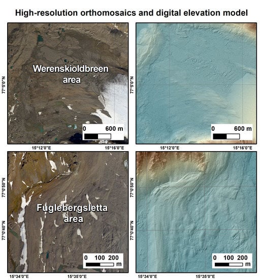
4.1. Digital Elevation Model and Orthomosaics Based on Aerial Imageries

4.1.1. Fuglebergsletta

As a result of aligning the images, 325 from 326 were correctly aligned. Camera locations and image overlaps are presented in Figure 3A. Details on data processing are shown in Table 1. The final resolution of the DEM equals 0.169 m and the point density was 35.2 points/m2. The root mean square error for all 27 GCP locations calculated by the software was 0.0018 m. Based on the improved dense clouds, digital elevation models were generated. The DEM was exported to raster format with 0.169 m resolution, the best possible resolution with this software, to increase the possibility of mapping even the smallest geomorphological features [16]. The vertical quality of the DEM was assessed based on 29 GCPs that were not used in the aerotriangulation process (Figure 4A). The standard deviation equaled 0.14 m, with a mean value of −0.22 m and a median value of −0.19 m. The maximal vertical error of the DEM equaled 0.54 m. There is a small systematic error in the DEM. In general, the elevation of the DEM generated in Agisoft is slightly higher than the measured elevation of the checkpoints.
After the final colour calibration of the entire dataset, an orthomosaic was produced (Figure 4B). The resolution of the orthomosaic was two times higher than the DEMs, which were the basis for its creation, and equalled 0.0843 m. The horizontal accuracy of the orthomosaic was estimated based on the same GCP points as those used for the DEM accuracy assessment. The standard deviation of the horizontal accuracy equalled 0.10 m, with a mean value of −0.12 m and a median value of −0.10 m.
In the low-image-overlap areas, the insufficient color blending over merged images may be noticeable. Even using color and white balance calibration in postprocessing, this effect was difficult to eliminate. For flat areas located below c. 140 m a.s.l., the applied flight parameters were sufficient to assemble the models. However, the mountain slopes and peaks on both study sites were characterized by either insufficient or a complete lack of coverage (Figure 3A). This resulted in broad blank areas (Figure 4) in the DEM and orthomosaic. Parts of the model composed only of a pair of images occasionally presented coarse graining or a deep generalization of elevation data (Figure 5A). Similar effects occur even with multiple overlaps on watercourses, surface water (Figure 5A) and the sea. For this reason, the DEM shows negative point values, reaching –15 m. Artefacts were also generated by moving objects, such as animals (Figure 5B).

4.1.2. Werenskioldbreen Area

As a result of aligning the images, 285 out of 296 photos for Werenskioldbreen were aligned correctly. Both the automatic and manual alignment functions failed to merge ten images representing the southern part of the glacier. It was caused by low overlap over the Angellfjellet ridge (594 m a.s.l.) and partial cloud cover over this area, making it difficult to detect tie points correctly. Camera locations and image overlaps for the second area are presented in Figure 3B. Details on data processing are described in Table 1. The final resolution of the DEM equals 0.174 m and the point density is 33 points/m2. The root mean square error for three points used in aerotriangulation was 0.0011 m. The resolution of the DEM in raster format and orthomosaics generated for the zone was 0.174 and 0.087 m, respectively (Figure 6). The resolution difference between orthomosaics for Werenskioldbreen and Fuglebergsletta was caused by the variation between mean ground level and flight altitude. Similar to the DEM for Fuglebergsletta, noises over water bodies (e.g., Figure 5C) are also present for the Werenskioldbreen area.
No checkpoints were applied to assess the final absolute vertical accuracy of the DEM and horizontal accuracy of the orthomosaic. However, we compared the DEM and orthomosaic generated using three points in aerotriangulation and without using any GCP. Results show significant improvement of the former products. The DEM accuracy measured over the three GCPs increased from 1.77 m to 0.22 m. The horizontal accuracy of the orthomosaic increased from 1.29 m to around 0.1 m (the orthomosaic was shifted towards the southeast).

4.2. TLS

In this study, we only used point clouds within 3 km from the laser scanner position (Figure 7; see Chapter 3.2.2). The four scans were registered using nearly 540,000 plane patches detected throughout the area (Figure 7). The final point cloud had over 117 million points, with a density of around 500–600 thousand points per m2 in the near-field region of the scans and just a few points per m2 at the distance of 3 km from the scanner. The RMS error obtained during the relative registration of all four point clouds was 0.09 m.
The final point cloud was then georeferenced utilizing 20 RIEGL reflectors (Figure 7C), with an RMS error of 0.13 m. The lowest accuracy in the northerly direction (0.2 to 0.3 m) was noticed for the two lateral scans, numbers 2 and 4. The lowest accuracy in the easterly direction was for scan number 1 (0.21 to 0.25 m). Height accuracy was high for all scans (of order 0.01–0.05 m).
The georeferenced cloud point was next filtered using an Octree algorithm in RiSCAN Pro 2.12.1 with a cell length of 0.16 m and converted into the raster format in ArcGIS (Esri, California) with 0.16 m resolution. As the areas of DEM interpolated in the shadow are characterized by lower accuracy, NoData values were assigned to the raster where holes in the data were present. Therefore, the DEM contains data gaps and keeps information only at spots measured directly by the laser scanner. The vertical quality of the TLS-based DEM was assessed based on the 19 independent points (Figure 7B). The standard deviation equalled 0.31 m and median value −0.19 m. The maximal vertical error of the DEM was 0.93 m.

4.3. Integration of Aerial DEM with TLS

The resulting M3C2-based point cloud distances are presented in Figure 8. Generally, the differences between both point clouds over the surveyed area were in the range of the vertical accuracy of the product (SD equalled 0.14 m and 0.31 m for aerial and TLS data, respectively). The map of surface differences shows local changes ranging from −4 m to 2 m (Figure 8A). The largest recorded differences, up to −4 m, are noted over the gullies and depressions filled by snow in 2020. Therefore, before integrating both DEMs, all areas covered by snow were removed from the aerial-based point cloud (Figure 8B,C). We also documented the erosion of lateral moraine of Hansbreen (around −0.7 m), which consists of an ice core covered with debris, as well as erosion along the shoreline. There are elevation changes of about 1 m concentrated over the mountain slope in the western part of the analyzed area. Numerous large boulders probably affect the quality and accuracy of the TLS-based DEM in that zone. As the scanner was located on marine terraces, around 300 m below, the laser beam was directed significantly upwards, and reflected off the wall of these boulders, rather than the top. Regardless of these local differences, we combined both DEMs into one continuous product. The final dataset (Figure 8D) is composed of a mosaic of two DEMs in raster format. All data gaps and snow areas in the aerial-based DEM were filled with the TLS-based DEM, with a blending option over a two-meter seamline. Moreover, we interpolated DEM values for a few remaining holes, where no data from both campaigns were present and interpolation of the DEM was made under the building and infrastructure of PPS (Figure 8D).

5. Discussion

The two approaches to acquiring the terrain data discussed in this paper are helpful in studying the landform topography and different environmental processes in the Hornsund area. However, both technologies have their limitations. The best vertical accuracy was noted for the aerial-based DEM. However, the limited sidelap of the mission caused data gaps in DEM over mountain slopes. Such settings should be considered when planning subsequent missions in the future, especially when the area of interest is land relief of the mountain regions.
Further, as GCPs and checkpoints were not established prior to the photograph surveys, we chose large, outsize boulders to serve as calibration and validation points [47,48]. Using such existing ‘stable’ features is a limitation of studies that use photogrammetric methods to produce DEMs [48]. For the first studied zone, Fuglebergsletta, we used enough GCPs to generate the DEM and orthomosaic and assess their accuracy. For the Werenskioldbreen area, only three points would have been used to create the DEM and orthomosaic. Thus, more significant distortions in the northern part of the study must be expected due to the lack of GCPs in that part of the model. Notwithstanding this, we generated the best products with the best resolution and accuracy for the Hornsund area. Further, it is possible to supplement them with better-representing GCPs and recalculate the dataset in the future. We would also like to underline here that regardless of the vertical accuracy of DEMs, the very high resolution of the DEMs gives the possibility to map even the smallest geomorphological features, compute geomorphometric indices and carefully estimate geomorphometric parameters [16].
The accuracy of the TLS-based DEM is slightly lower than the aerial-based product. One of the properties that strongly influenced the long-range TLS was an inhomogeneous point density throughout the area of interest and positional uncertainty due to the laser beam width [22,30,42,46]. Laser footprint size at long 3 km distances equals around 0.36 m. Furthermore, on inclined surfaces the laser footprint becomes deformed to an ellipse [22]. The uncertainty caused by these large footprints are not yet quantified, but is expected to be in the order of decimeters and strongly depends on the distance from the scanner to the surface [27]. Laser scanner data are susceptible to data gaps in locations not in the direct line-of-sight of the scanner, resulting in ‘range shadows’ which inherently added uncertainty to the derived product [22,38,42,45,49]. Further, the configuration of the scan position and Riegl flat reflectors [30] was limited by terrain conditions, which would increase the error in relative alignment and absolute registration of scans. Considering all these limitations, the final vertical and horizontal accuracy of the TLS-based DEM of order 0.30 m is not unexpected to be in the lower-decimeter range [27] and is the best possible for the complex natural terrain. The DEM at interpolated areas has a quality lower than estimated in the study. In the future, viewshed analysis before TLS fieldwork could remove the shadowing effect [50,51] and improve the accuracy of the data.
The snow cover present in the aerial imagery taken in 2020 and data gaps in both point clouds led us to integrate both datasets [32,52]. Usually, within point-cloud-based strategies, the data acquired in at least two epochs are used to determine the geometric changes between them [30,43,44,52]. Here, apart from the accuracy assessment, we compared and combined the data acquired within one year. The distances between both point clouds were distributed unevenly over the whole area. The differences lower than the vertical accuracy of DEM (SD = 0.31 m) indicated the stable area. The final DEM for Fuglebergsletta was composed of the aerial-based DEM, with data gaps and the snow-covered regions filled by TLS data. One needs to keep in mind that the expected accuracy of such a product is lower than singular point clouds acquired over two years, as the combined DEM comes from the datasets collected in 2020 and 2021. Merging two DEMs from two different years is challenging, as the study area is undergoing continuous changes in land relief. However, temporal changes in most of the area are below the accuracy of both DEMs, and therefore the DEM can be successfully applied to hydrological, glaciological, biological and geomorphometric studies, when observed changes are larger than the accuracy of the DEM. In other words, the merged DEM that we have generated represents the topography of the region’s independent annual surface elevation changes, since the incorporated data were collected during the following two years. In the process of merging two datasets, the annual elevation changes may not reflect in the resulting DEM because of suppression of high-density elevation data recorded from TLS and photogrammetric methods [53,54].
To conclude, the final point clouds, DEMs and orthomosaic are the best terrain products with the highest spatial resolution for the Hornsund area and can be used for further environmental studies. They allowed us to identify local geomorphic processes, such as melting of ice cores at the periglacial area or shoreline erosion. However, for studies aiming to identify changes within a specified time range or slow geomorphometric processes on slopes, we recommend using data from the same types of sources (aerial/TLS) or stemming from a more extended period, such as DEMs generated from aerial imagery taken in 2011 [17]. In addition, we would like to underline here that all the DEMs should be first co-registered [55,56] and the final error must be defined to differentiate between real changes and data noise [22]. This is especially important for the DEM of the Werenskioldbreen area, as only three GCPs located along an almost-straight line were used in the data processing. This suggests that despite the high relative accuracy of the DEM, the absolute accuracy could be lower and decrease with the distance from measured GCPs; therefore, co-registration is needed when comparing with the other data.

6. Conclusions

The Hornsund area is the site in the focus of several studies due to the vicinity of the Polish Polar Station. It is a complex terrain under constant changes, although it lacks repeated datasets with spatial resolution high enough to map even the smallest geomorphological features. In the present study we derived aerial-based DEMs, TLS-based DEMs and orthomosaics, and assessed their accuracy and usefulness for further environmental studies.
Aerial data provided by SIOS were used to generate the DEMs and orthomosaics for the Fuglebergsletta and Werenskioldbreen areas. The products lack gaps over the mountain slopes due to the low sidelap during the flight. Nevertheless, the derived DEM has sufficient quality to study different geomorphometric features. Long-range TLS, despite limitations such as data gaps, complex terrain which limits scan positions and large laser footprint sizes at long distances, can also serve for future analysis of the different geomorphological processes. In particular, the area close to the scanner position with very dense point clouds can be used for future studies of 3D displacements and minor geomorphological features.
This work demonstrates that combining other techniques could be an option, especially in remote polar areas, when data acquisition depends on many factors. In order to remove the aforementioned holes in the datasets from aerial and TLS surveys, we integrated both DEMs over the area close to the Polish Polar Station. Comparison of the point clouds revealed a few small zones under local geomorphic processes, such as the melting of ice cores at the periglacial zone and changes along the shoreline. The differences in both products over the rest of the area were generally lower than the accuracy of both DEMs. This allowed us to combine the data and create the final continuous DEM without gaps for the Fuglebergsletta area. After the proper co-registration, all point clouds and DEMs can be successfully applied in further studies of landform evolution and hydrological, geomorphometric and other processes in the region.

Author Contributions

Conceptualization, M.B.; methodology, M.B., M.L., A.S. and S.D.J.; flight planning, mission execution and aerial data acquisition A.S., S.D.J., M.L. and M.B.; data curation, M.B. and M.L.; writing—original draft preparation, M.B. and M.L.; writing—review and editing, S.D.J. and A.S. All authors have read and agreed to the published version of the manuscript.

Funding

The fieldwork has been financed by the Centre for Polar Studies of the University of Silesia, Poland. The SIOS KC would like to acknowledge the support from the Research Council of Norway (RCN) through projects No. 291644 & No. 269927 and the Norwegian Space Agency (NoSA) through contract No. NIT 12.20.5. The Hyperspectral sensor onboard the Dornier aircraft is funded by the SIOS-InfraNor project (No. 269927).

Informed Consent Statement

Not applicable.

Data Availability Statement

Publicly available datasets were analyzed in this study. This data can be found here: DEM for Fuglebergsletta area from Dornier images: https://ppdb.us.edu.pl/geonetwork/srv/eng/catalog.search#/metadata/69987fe3-f0ed-4fdc-b597-41dd5ae7d21a (accessed on 23 December 2021), Orthomosaic for Fuglebergsletta area from Dornier images: https://ppdb.us.edu.pl/geonetwork/srv/eng/catalog.search#/metadata/9b980572-2bcb-401f-a2e6-2a7a16428dd7 (accessed on 23 December 2021), DEM for Werenskioldbreen area from Dornier images: https://ppdb.us.edu.pl/geonetwork/srv/eng/catalog.search#/metadata/87a556ed-6b8f-4d06-9c20-1a5b6b23d280 (accessed on 23 December 2021), Orthomosaic for Werenskioldbreen area from Dornier images: https://ppdb.us.edu.pl/geonetwork/srv/eng/catalog.search#/metadata/c99085cb-7e4c-43dd-866b-f2f909b44937 (accessed on 23 December 2021), Terrestrial laser scanner (TLS) data for Fuglebergsletta area: https://ppdb.us.edu.pl/geonetwork/srv/eng/catalog.search#/metadata/8bb03c41-35de-46b5-87c1-bd6c82fa2914 (accessed on 23 December 2021), Combined DEM for Fuglebergsletta area from Dornier images and terrestrial laser scanner (TLS): https://ppdb.us.edu.pl/geonetwork/srv/eng/catalog.search#/metadata/eec5dd69-20c0-46c6-aa16-8bb9cece3e85 (accessed on 23 December 2021).

Acknowledgments

The authors would like to acknowledge the Institute of Geophysics PAS and project POLARPOL for enabling the use of terrestrial laser scanner Riegl VZ®-6000. The studies were carried out as part of the scientific activity of the Centre for Polar Studies (University of Silesia in Katowice) with the use of research and logistic equipment (GNSS receivers and supporting equipment) of the Polar Laboratory of the University of Silesia in Katowice. The authors would like to thank Jacek Jania and participants of the polar expedition of the University of Silesia in Katowice 2021 for assistance with the fieldwork. Thanks are directed to the staff of the Institute of Geophysics PAS and the Polish Polar Station, Hornsund for assistance during the field campaign. All the authors acknowledge the SIOS Knowledge Centre (SIOS-KC) for funding and conducting flight campaigns over the study area.

Conflicts of Interest

The authors declare no conflict of interest.

References

  1. Grabiec, M.; Puczko, D.; Budzik, T.; Gajek, G. Snow distribution patterns on Svalbard glaciers derived from radio-echo soundings. Pol. Polar Res. 2011, 32, 393–421. [Google Scholar] [CrossRef] [Green Version]
  2. Grabiec, M.; Jania, J.A.; Puczko, D.; Kolondra, L.; Budzik, T. Surface and bed morphology of Hansbreen, a tidewater glacier in Spitsbergen. Pol. Polar Res. 2012, 33, 111–138. [Google Scholar] [CrossRef]
  3. Ziaja, W.; Ostafin, K. Landscape–seascape dynamics in the isthmus between Sørkapp Land and the rest of Spitsbergen: Will a new big Arctic island form? AMBIO 2015, 44, 332–342. [Google Scholar] [CrossRef] [Green Version]
  4. Błaszczyk, M.; Jania, J.A.; Ciepły, M.; Grabiec, M.; Ignatiuk, D.; Kolondra, L.; Kruss, A.; Luks, B.; Moskalik, M.; Pastusiak, T.; et al. Factors Controlling Terminus Position of Hansbreen, a Tidewater Glacier in Svalbard. J. Geophys. Res. Earth Surf. 2021, 126, e2020JF005763. [Google Scholar] [CrossRef]
  5. Majchrowska, E.; Ignatiuk, D.; Jania, J.; Marszałek, H.; Wąsik, M. Seasonal and interannual variability in runoff from the Werenskioldbreen catchment, Spitsbergen. Pol. Polar Res. 2015, 36, 197–224. [Google Scholar] [CrossRef] [Green Version]
  6. Stachnik, Ł.; Majchrowska, E.; Yde, J.C.; Nawrot, A.P.; Cichała-Kamrowska, K.; Ignatiuk, D.; Piechota, A. Chemical denudation and the role of sulfide oxidation at Werenskioldbreen, Svalbard. J. Hydrol. 2016, 538, 177–193. [Google Scholar] [CrossRef] [Green Version]
  7. Wawrzyniak, T.; Osuch, M.; Nawrot, A.; Napiorkowski, J.J. Run-off modelling in an Arctic unglaciated catchment (Fuglebekken, Spitsbergen). Ann. Glaciol. 2017, 58, 36–46. [Google Scholar] [CrossRef] [Green Version]
  8. Osuch, M.; Wawrzyniak, T.; Nawrot, A. Diagnosis of the hydrology of a small Arctic permafrost catchment using HBV conceptual rainfall-runoff model. Hydrol. Res. 2019, 50, 459–478. [Google Scholar] [CrossRef] [Green Version]
  9. Kępski, D.; Luks, B.; Migała, K.; Wawrzyniak, T.; Westermann, S.; Wojtuń, B. Terrestrial Remote Sensing of Snowmelt in a Diverse High-Arctic Tundra Environment Using Time-Lapse Imagery. Remote Sens. 2017, 9, 733. [Google Scholar] [CrossRef] [Green Version]
  10. Dolnicki, P.; Grabiec, M.; Puczko, D.; Gawor, Ł.; Budzik, T.; Klementowski, J. Variability of temperature and thickness of permafrost active layer at coastal sites of Svalbard. Pol. Polar Res. 2013, 34, 353–374. [Google Scholar] [CrossRef] [Green Version]
  11. Glazer, M.; Dobiński, W.; Marciniak, A.; Majdański, M.; Błaszczyk, M. Spatial distribution and controls of permafrost development in non-glacial Arctic catchment over the Holocene, Fuglebekken, SW Spitsbergen. Geomorphology 2020, 358, 107128. [Google Scholar] [CrossRef]
  12. Zagórski, P.; Rodzik, J.; Moskalik, M.; Strzelecki, M.C.; Lim, M.; Błaszczyk, M.; Promińska, A.; Kruszewski, G.; Styszyńska, A.; Malczewski, A. Multidecadal (1960–2011) shoreline changes in Isbjørnhamna (Hornsund, Svalbard). Pol. Polar Res. 2015, 36, 369–390. [Google Scholar] [CrossRef]
  13. Senderak, K.; Kondracka, M.; Gądek, B. Talus slope evolution under the influence of glaciers with the example of slopes near the Hans Glacier, SW Spitsbergen, Norway. Geomorphology 2017, 285, 225–234. [Google Scholar] [CrossRef]
  14. Strzelecki, M.C.; Szczuciński, W.; Dominiczak, A.; Zagórski, P.; Dudek, J.; Knight, J. New fjords, new coasts, new landscapes: The geomorphology of paraglacial coasts formed after recent glacier retreat in Brepollen (Hornsund, southern Svalbard). Earth Surf. Process. Landf. 2020, 45, 1325–1334. [Google Scholar] [CrossRef] [Green Version]
  15. Sułowicz, S.; Bondarczuk, K.; Ignatiuk, D.; Jania, J.A.; Piotrowska-Seget, Z. Microbial communities from subglacial water of naled ice bodies in the forefield of Werenskioldbreen, Svalbard. Sci. Total Environ. 2020, 723, 138025. [Google Scholar] [CrossRef] [PubMed]
  16. Marotta, F.; Teruggi, S.; Achille, C.; Vassena, G.P.; Fassi, F. Integrated Laser Scanner Techniques to Produce High-Resolution DTM of Vegetated Territory. Remote Sens. 2021, 13, 2504. [Google Scholar] [CrossRef]
  17. Błaszczyk, M.; Ignatiuk, D.; Grabiec, M.; Kolondra, L.; Laska, M.; Decaux, L.; Jania, J.; Berthier, E.; Luks, B.; Barzycka, B.; et al. Quality Assessment and Glaciological Applications of Digital Elevation Models Derived from Space-Borne and Aerial Images over Two Tidewater Glaciers of Southern Spitsbergen. Remote Sens. 2019, 11, 1121. [Google Scholar] [CrossRef] [Green Version]
  18. Jawak, S.D.; Andersen, B.N.; Pohjola, V.A.; Godøy, Ø.; Hübner, C.; Jennings, I.; Ignatiuk, D.; Holmén, K.; Sivertsen, A.; Hann, R.; et al. SIOS’s Earth Observation (EO), Remote Sensing (RS), and Operational Activities in Response to COVID-19. Remote Sens. 2021, 13, 712. [Google Scholar] [CrossRef]
  19. Buckley, S.J.; Schwarz, E.; Terlaky, V.; Howell, J.A.; Arnott, R.W.C. Terrestrial laser scanning combined with photogrammetry for digital outcrop modelling. Int. Arch. Photogramm. Remote Sens. Spat. Inf. Sci. 2009, 38, 75–80. [Google Scholar]
  20. Prokop, A.; Delaney, C. A high resolution approach to defining spatial snow height distribution in avalanche release zones for dynamic avalanche modeling. In Proceedings of the ISSW 2010, Lake Tahoe, CA, USA, 17–22 October 2010; pp. 839–845. [Google Scholar]
  21. Sima, A.A.; Buckley, S.J.; Schneider, D.; Howell, J.A. An improved workflow for image- and laser-based virtual geological outcrop modelling. Int. Arch. Photogramm. Remote Sens. Spat. Inf. Sci. 2010, 3, 115–119. [Google Scholar]
  22. Fey, C.; Wichmann, V. Long-range terrestrial laser scanning for geomorphological change detection in alpine terrain—Handling uncertainties. Earth Surf. Process. Landf. 2017, 42, 789–802. [Google Scholar] [CrossRef]
  23. Müller, D.; Walter, T.R.; Schöpa, A.; Witt, T.; Steinke, B.; Gudmundsson, M.T.; Dürig, T. High-Resolution Digital Elevation Modeling from TLS and UAV Campaign Reveals Structural Complexity at the 2014/2015 Holuhraun Eruption Site, Iceland. Front. Earth Sci. 2017, 5, 59. [Google Scholar] [CrossRef] [Green Version]
  24. Xu, C.; Li, Z.; Wang, F.; Li, H.; Wang, W.; Wang, L.I.N. Using an ultra-long-range terrestrial laser scanner to monitor the net mass balance of Urumqi Glacier No. 1, eastern Tien Shan, China, at the monthly scale. J. Glaciol. 2017, 63, 792–802. [Google Scholar] [CrossRef]
  25. Wang, F.; Xu, C.; Li, Z.-Q.; Anjum, M.N.; Wang, L. Applicability of an ultra-long-range terrestrial laser scanner to monitor the mass balance of Muz Taw Glacier, Sawir Mountains, China. Sci. Cold Arid Reg. 2018, 10, 47–54. [Google Scholar]
  26. Fischer, M.; Huss, M.; Kummert, M.; Hoelzle, M. Application and validation of long-range terrestrial laser scanning to monitor the mass balance of very small glaciers in the Swiss Alps. Cryosphere 2016, 10, 1279–1295. [Google Scholar] [CrossRef] [Green Version]
  27. Voordendag, A.B.; Goger, B.; Klug, C.; Prinz, R.; Rutzinger, M.; Kaser, G. Automated and permanent long-range terrestrial laser scanning in a high mountain environment: Setup and first results. ISPRS Ann. Photogramm. Remote Sens. Spat. Inf. Sci. 2021, 2, 153–160. [Google Scholar] [CrossRef]
  28. Prantl, H.; Nicholson, L.; Sailer, R.; Hanzer, F.; Juen, I.F.; Rastner, P. Glacier Snowline Determination from Terrestrial Laser Scanning Intensity Data. Geosciences 2017, 7, 60. [Google Scholar] [CrossRef] [Green Version]
  29. LeWinter, A.; Finnegan, D.C.; Hamilton, G.S.; Stearns, L.A.; Gadomski, P.J. Continuous Monitoring of Greenland Outlet Glaciers Using an Autonomous Terrestrial LiDAR Scanning System: Design, Development and Testing at Helheim Glacier. In Proceedings of the AGU Fall Meeting, San Fracnisco, CA, USA, 15–16 December 2014. [Google Scholar]
  30. Pfeiffer, J.; Zieher, T.; Bremer, M.; Wichmann, V.; Rutzinger, M. Derivation of Three-Dimensional Displacement Vectors from Multi-Temporal Long-Range Terrestrial Laser Scanning at the Reissenschuh Landslide (Tyrol, Austria). Remote Sens. 2018, 10, 1688. [Google Scholar] [CrossRef] [Green Version]
  31. Dietrich, A.; Krautblatter, M. Deciphering controls for debris-flow erosion derived from a LiDAR-recorded extreme event and a calibrated numerical model (Roßbichelbach, Germany). Earth Surf. Process. Landf. 2019, 44, 1346–1361. [Google Scholar] [CrossRef]
  32. Pagano, M.; Palma, B.; Ruocco, A.; Parise, M. Discontinuity Characterization of Rock Masses through Terrestrial Laser Scanner and Unmanned Aerial Vehicle Techniques Aimed at Slope Stability Assessment. Appl. Sci. 2020, 10, 2960. [Google Scholar] [CrossRef]
  33. Milenković, M.; Pfeifer, N.; Glira, P. Applying Terrestrial Laser Scanning for Soil Surface Roughness Assessment. Remote Sens. 2015, 7, 2007. [Google Scholar] [CrossRef] [Green Version]
  34. Błaszczyk, M.; Jania, J.A.; Kolondra, L. Fluctuations of tidewater glaciers in Hornsund Fjord (Southern Svalbard) since the beginning of the 20th century. Pol. Polar Res. 2013, 34, 327–352. [Google Scholar] [CrossRef]
  35. Jania, J. Dynamiczne Procesy Glacjalne na Południowym Spitsbergenie (w Świetle Badań Fotointerpretacyjnych i Fotogrametrycznych). (Dynamic Glacial Processes in South Spitsbergen [in Light of Photo Interpretation and Photogrammetric Research]); Wydawnictwo Uniwersytetu Śląskiego: Katowice, Poland, 1988. [Google Scholar]
  36. Westoby, M.J.; Brasington, J.; Glasser, N.F.; Hambrey, M.J.; Reynolds, J.M. ‘Structure-from-Motion’ photogrammetry: A low-cost, effective tool for geoscience applications. Geomorphology 2012, 179, 300–314. [Google Scholar] [CrossRef] [Green Version]
  37. Hann, R.; Altstädter, B.; Betlem, P.; Deja, K.; Dragańska-Deja, K.; Ewertowski, M.; Hartvich, F.; Jonassen, M.; Lampert, A.; Laska, M.; et al. Scientific Applications of Unmanned Vehicles in Svalbard. In Moreno-Ibáñez et al (eds) SESS Report 2020; Svalbard Integrated Arctic Earth Observing System: Longyearbyen, Svalbard and Jan Mayen, 2021. [Google Scholar]
  38. Buckley, S.J.; Howell, J.A.; Enge, H.D.; Kurz, T.H. Terrestrial laser scanning in geology: Data acquisition, processing and accuracy considerations. J.Geol. Soc. 2008, 165, 625. [Google Scholar] [CrossRef]
  39. Riegl. Available online: http://www.riegl.com/nc/products/terrestrial-scanning/produktdetail/product/scanner/33/ (accessed on 16 December 2021).
  40. Kersten, T.P.; Mechelke, K.; Lindstaedt, M.; Sternberg, H. Methods for Geometric Accuracy Investigations of Terrestrial Laser Scanning Systems. Photogramm. Fernerkund. Geoinf. 2009, 4, 301–315. [Google Scholar] [CrossRef] [PubMed]
  41. Buchroithner, M.F.; Gaisecker, T. Ice surface changes in Eisriesenwelt (Salzburg, Austria) based on LIDAR measurements between 2017 and 2020. Die Höhle 2020. Available online: http://www.riegl.com/media-events/projects/terrestrial-scanning/project/manfred-f-buchroithner-thomas-gaisecker-ice-surface-changes-in-eisriesenwelt-salzburg-austria/ (accessed on 23 December 2021).
  42. Lague, D.; Brodu, N.; Leroux, J. Accurate 3D comparison of complex topography with terrestrial laser scanner: Application to the Rangitikei canyon (N-Z). ISPRS J. Photogramm. Remote Sens. 2013, 82, 10–26. [Google Scholar] [CrossRef] [Green Version]
  43. Anders, K.; Marx, S.; Boike, J.; Herfort, B.; Wilcox, E.J.; Langer, M.; Marsh, P.; Höfle, B. Multitemporal terrestrial laser scanning point clouds for thaw subsidence observation at Arctic permafrost monitoring sites. Earth Surf. Process. Landf. 2020, 45, 1589–1600. [Google Scholar] [CrossRef]
  44. Holst, C.; Janßen, J.; Schmitz, B.; Blome, M.; Dercks, M.; Schoch-Baumann, A.; Blöthe, J.; Schrott, L.; Kuhlmann, H.; Medic, T. Increasing Spatio-Temporal Resolution for Monitoring Alpine Solifluction Using Terrestrial Laser Scanners and 3D Vector Fields. Remote Sens. 2021, 13, 1192. [Google Scholar] [CrossRef]
  45. O’Banion, M.S.; Olsen, M.J.; Hollenbeck, J.P.; Wright, W.C. Data Gap Classification for Terrestrial Laser Scanning-Derived Digital Elevation Models. ISPRS Int. J. Geo-Inform. 2020, 9, 749. [Google Scholar] [CrossRef]
  46. Lichti, D.D.; Gordon, S.J. Error propagation in directly georeferenced terrestrial laser scanner point clouds for cultural heritage recording. In Proceedings of the FIG Working Week 2004, Athens, Greece, 22–27 May 2004. [Google Scholar]
  47. Staines, K.E.H.; Carrivick, J.L.; Tweed, F.S.; Evans, A.J.; Russell, A.J.; Jóhannesson, T.; Roberts, M. A multi-dimensional analysis of pro-glacial landscape change at Sólheimajökull, southern Iceland. Earth Surf. Process. Landf. 2015, 40, 809–822. [Google Scholar] [CrossRef]
  48. Tonkin, T.N.; Midgley, N.G.; Cook, S.J.; Graham, D.J. Ice-cored moraine degradation mapped and quantified using an unmanned aerial vehicle: A case study from a polythermal glacier in Svalbard. Geomorphology 2016, 258, 1–10. [Google Scholar] [CrossRef] [Green Version]
  49. Nesbit, P.R.; Hugenholtz, C.H. Enhancing UAV–SfM 3D Model Accuracy in High-Relief Landscapes by Incorporating Oblique Images. Remote Sens. 2019, 11, 239. [Google Scholar] [CrossRef] [Green Version]
  50. Starek, M.J.; Chu, T.; Mitasova, H.; Harmon, R.S. Viewshed simulation and optimization for digital terrain modelling with terrestrial laser scanning. Int. J. Remote Sens. 2020, 41, 6409–6426. [Google Scholar] [CrossRef]
  51. Heritage, G.L.; Milan, D.J.; Large, A.R.G.; Fuller, I.C. Influence of survey strategy and interpolation model on DEM quality. Geomorphology 2009, 112, 334–344. [Google Scholar] [CrossRef]
  52. Belmonte, A.; Sankey, T.; Biederman, J.; Bradford, J.; Goetz, S.; Kolb, T. UAV-Based Estimate of Snow Cover Dynamics: Optimizing Semi-Arid Forest Structure for Snow Persistence. Remote Sens. 2021, 13, 1036. [Google Scholar] [CrossRef]
  53. Jawak, S.D.; Luis, A.J. Synergistic use of multitemporal RAMP, ICESat and GPS to construct an accurate DEM of the Larsemann Hills region, Antarctica. Adv. Space Res. 2012, 50, 457–470. [Google Scholar] [CrossRef]
  54. Jawak, S.D.; Luis, A.J. Synergetic merging of Cartosat-1 and RAMP to generate improved digital elevation model of Schirmacher Oasis, east Antarctica. Int. Arch. Photogramm. Remote Sens. Spat. Inf. Sci. 2014, 40, 517. [Google Scholar] [CrossRef] [Green Version]
  55. Berthier, E.; Arnaud, Y.; Kumar, R.; Ahmad, S.; Wagnon, P.; Chevallier, P. Remote sensing estimates of glacier mass balances in the Himachal Pradesh (Western Himalaya, India). Remote Sens. Environ. 2007, 108, 327–338. [Google Scholar] [CrossRef] [Green Version]
  56. Nuth, C.; Schuler, T.V.; Kohler, J.; Altena, B.; Hagen, J.O. Estimating the long-term calving flux of Kronebreen, Svalbard, from geodetic elevation changes and mass-balance modeling. J. Glaciol. 2012, 58, 119–133. [Google Scholar] [CrossRef] [Green Version]
Figure 1. Location of the study area. The blue outlines represent the extent of aerial imagery acquired during the crewed aircraft campaign in 2020; the red polygon presents the range of data taken by terrestrial scanner Riegl VZ-6000 in 2021; the red asterisks illustrate the positions of the laser scanner; the orange dots represent ground control points and the yellow dots represent checkpoints measured by GPS in 2021; the blue rectangle presents the location of the Polish Polar Station, Hornsund.
Remotesensing 14 00601 g001
Figure 2. Processing workflow for airborne data and terrestrial laser scanning (TLS).
Remotesensing 14 00601 g002
Figure 3. Camera locations (black dots) and image numbers and overlaps over Fuglebergsletta (A) and Werenskioldbreen area (B).
Remotesensing 14 00601 g003
Figure 4. Digital Elevation Model (A) and orthomosaic (B) for the Fuglebergsletta area. Orange points represent GCPs used during processing in Agisoft, while yellow points served as checkpoints to estimate the quality of the products.
Remotesensing 14 00601 g004
Figure 5. Artefacts described in the text: coarse graining or a deep generalization of elevation data (A), artefacts generated by reindeers (B) and noises over water bodies (A,C).
Remotesensing 14 00601 g005
Figure 6. Digital Elevation Model (A) and orthomosaic (B) for the Werenskioldbreen area. Orange points represent GCPs used in processing in Agisoft.
Remotesensing 14 00601 g006
Figure 7. Terrestrial laser scanning data over the study area. The yellow polygon in (A) indicates the area covered by all scans, while the brown polygon presents the data range used in the registration procedure. Yellow asterisks in (B) illustrate the positions of the laser scanner. Orange and yellow dots represent GCPs and checkpoints that served to estimate the quality of the raster DEM generated from TLS data. Red dots in (C) present the example positioning of the RIEGL reflectors regarding the scanner position.
Remotesensing 14 00601 g007
Figure 8. Comparison of the multitemporal point clouds: aerial-based point cloud from images taken in 2020 and TLS-based point cloud collected in 2021. (A) M3C2-calculated distance between aerial-based and TLS dataset; (B) orthomosaic presenting data gaps and snow cover over the land in 2020; (C) vertical difference of the point clouds with snow cover area eliminated from further data integration; (D) the final DEM integrated from both DEMs. Black polygons present the areas where DEM was interpolated.
Remotesensing 14 00601 g008
Table 1. Processing settings and final resolution of the products.
Image AlignmentDense CloudDepth Maps Filtering3D ModelDEMOrthomosaic
AccuracyTie PointsQualityPointsQualityFacesSizeResolutionSizeResolution
FuglebergslettaHigh356,693High1,074,237,705AggressiveHigh213,379,20973,519 × 38,7690.169 m106,313 × 50,3810.0843 m
WerenskioldbreenHigh323,830High959,690,194AggressiveHigh191,045,20361,565 × 45,5920.174 m81,027 × 53,5110.087 m
Publisher’s Note: MDPI stays neutral with regard to jurisdictional claims in published maps and institutional affiliations.

