Article

Exploring Park Visit Variability Using Cell Phone Data in Shenzhen, China

1
Shenzhen Institute of Advanced Technology, Chinese Academy of Sciences, Shenzhen 518055, China
2
School of Software Engineering, University of Science and Technology of China, Hefei 230026, China
*
Author to whom correspondence should be addressed.
Remote Sens. 2022, 14(3), 499; https://doi.org/10.3390/rs14030499
Submission received: 24 December 2021 / Revised: 17 January 2022 / Accepted: 18 January 2022 / Published: 21 January 2022

Abstract

:
Exploring the spatiotemporal characteristics of park visitors and the “push and pull” factors that shape this mobility is critical to designing and managing urban parks to meet the demands of rapid urbanization. In this paper, 56 parks in Shenzhen were studied in 2019. First, cell phone signaling data were used to extract information on visitors’ departure locations and destination parks. Second, the bivariate Moran’s I and bivariate local Moran’s I (BiLISA) methods were used to identify the statistical correlation between the factors of the built environment and the park recreation trips. Finally, linear regression models were constructed to quantify the factors influencing the attractiveness of the park. Our study showed the following: (1) Recreation visitors at large parks varied significantly among population subgroups. Compared with younger adults, teenagers and older adults traveled lower distances and made fewer trips, and in particular, older adults of different genders differed significantly in park participation. (2) Recreational trips in large parks were related to the functional layout of the built environment around their residence. In areas with rich urban functions (e.g., southern Shenzhen), trips to large parks for leisure are more aggregated. (3) The findings reinforce the evidence that remote sensing data for urban vegetation can be an effective factor in characterizing park attractiveness, but the explanatory power of different vegetation data varies widely. Our study integrated the complementary human activity and remote sensing data to provide a more comprehensive understanding of urban park use and preferences. This will be important for future park planning.

1. Introduction

Urban parks are natural and artificial spaces with green potential in urban areas. They not only provide recreational services for residents, but also serve as important urban infrastructure for maintaining ecological balance and achieving sustainable urban development [1,2]. With accelerated urbanization and rapid population expansion, most urban outdoor spaces are crowded by high-rise buildings and dense road networks, which makes urban parks a major place for recreational activities. Exploring the spatial and temporal characteristics of recreation and leisure trips to parks and parks’ spatial connections with the built environment can provide a scientific basis for the planning and design of parks and policy-making on land use in the future. However, the relationship between park recreation and leisure trips and the urban environment has not been sufficiently investigated in Chinese cities [3].
Previous research on parks has focused on the urban ecological benefits from a landscape gardening perspective. In recent years, studies have gradually shifted to balance urban ecosystems and social welfare. Most studies have focused on community gardens, neighborhood parks, and street gardens [4,5,6,7] because of their walkability, abundance of recreational and sports facilities, and closeness to the elderly and children. For example, in Australia, it has been found that most users of small parks come from within a 500 m radius of the park [8]. In China, although the service radius of parks is not specified in the Standard for the Classification of Urban Green Space (CJJ/T85-2017) [9], some cities have park plans with 500 m as the service radius of parks to facilitate the travel of the surrounding residents. A recent study found that the actual service radius of large parks does not match, or far exceeds, the expected service radius planned by the government [10]. The reason for this was that travel distance is often less important for visitors who prefer large parks with specific facilities [11,12]. In addition, larger parks are considered to offer more ecological benefits, as well as more diverse and enjoyable outdoor activities than smaller community parks that are frequently used by surrounding residents [13]. Therefore, it is essential to investigate the usage characteristics of large urban parks from the actual recreational trips of visitors.
Spatial disparity in parks is common in many cities [14,15,16]. In Wuhan, China, the accessibility of park green spaces showed spatial polarization, with most of the underserved areas distributed in the eastern and southwestern parts of the city center [14]. In Fuzhou, China, the spatial distribution of effective park area presented a clear and notably decreasing trend from the urban center to its periphery [15]. The research results from Harbin showed that the supply of small parks is severely insufficient and the distribution of comprehensive parks is too concentrated [16]. Previous studies also have found that the supply of green space varies by race [4,17], gender, and age [18,19,20]. This, in turn, can affect the accessibility and balanced distribution of people’s park visits [19]. Accordingly, urban planning has placed great emphasis on the spatial analysis of the efficiency of use and serviceability provided by parks [21,22,23]. However, most studies have focused only on the neighborhood environment of parks and their differential characteristics, whereas fewer studies have examined long-distance large park visits and their spatial heterogeneity with the built environment [24]. Measuring the empirical relationship between park recreation trips and the built environment can provide a way to evaluate policies that stimulate or promote these factors and help improve our understanding of how to create enjoyable and healthy parks. A growing body of research has concluded that in addition to the socioeconomic attributes of individuals, park recreation trips are heavily influenced by their travel behavior and the surrounding built environment, such as population density, land-use diversity, and infrastructure availability [3,7,10]. However, there is still limited empirical evidence exploring the relationship between large parks and these factors. In most studies of environmental influences, researchers have used neighborhood-level characteristics (e.g., surrounding population density, the number of nearby bus stops, and the number of nearby commercial services) and park attributes (e.g., the number of facilities, internal accessibility) to examine the impact on park visitation [10,22,25,26]. In recent years, with the promotion of green and sustainable concepts, there has been a growing concern about ecological quality. From the existing studies, the ecological factors of parks such as vegetation were often analyzed as aesthetic features of parks [27], whereas studies on the correlation between vegetation quality and park visitation are still lacking [28,29]. In addition, from a provider’s perspective, recreation agencies require multiscale information to determine the location of facilities [24]. Research methods typically analyze urban built environment factors around parks at a fixed scale (e.g., 800 m [10]), whereas the evidence-based multiscale characterization of built environment factors around parks is scarce.
Traditional research methods for investigating park recreation tend to obtain data through surveys or observations, but their small and time-consuming sample sizes do not provide much information for park management at the city or regional level [30]. The recent boom in the use of geolocated social media (GSM) has created new ways to measure the characteristics of park visitation, such as geospatial data from Flickr photo-sharing sites [25,31], Gaode Maps [32], and other social media [33]. Weibo is one of the most used social media tools in China. Weibo was used in Li’s [34] study to evaluate the use of 13,759 parks in 287 cities in China, and they found that the density of the points of interest (POI) around parks had the most positive influence, whereas the park service area and landscape shape index (LSI) had a negative influence. Similarly, in Liu’s study [35,36], GSM data were used to analyze the spatial and temporal patterns of park visitation in central Shanghai and to measure and compare visitation to different types of parks. Compared with social media data, cell phone signal data have less group representativeness bias and higher temporal resolution and are, therefore, more suitable for measuring the usage patterns of large urban parks. Although multiple data sources have been used in park visitation studies [33,34,35,36], satellite data reflecting the quality of urban vegetation have rarely appeared in previous studies. They are more often used to analyze the relationship between resident health and the environment [37,38]. In the field of urban park recreation, the relationship between environmental status captured by satellite data and park visitation needs to be further validated.
In order to explore the factors related to the built environment and parks’ surroundings that can shape recreation mobility to parks, this study was conducted with 56 parks in Shenzhen in 2019. Combining data from cell phone signals, satellite-captured vegetation status, building heights, and urban POIs, we first analyzed the spatial and temporal characteristics of urban park visitation on weekdays, weekends, and holidays. Secondly, we used geostatistical methods to identify the spatial correlation between elements of the built environment and urban park trips. Finally, we constructed a set of multiple linear regression models to quantify the factors affecting park attractiveness, such as the park’s surroundings, its own conditions, and accessibility. We aimed to identify (1) the differences in park visitation characteristics between age groups at different times; (2) the spatial correlation characteristics between built-environment-related factors and recreation trips to parks; and (3) the factors of the parks’ surroundings that contribute significantly to park visitation.
The rest of the paper is organized as follows. Section 2 describes the study area and dataset. Section 3 describes the methods for extracting the locations of park visitors and the methods for analyzing the relationship that recreation trips to parks have with the built environment and the parks’ surrounding elements. Section 4 shows the experimental results. Section 5 discusses the data results. Section 6 presents our conclusions.

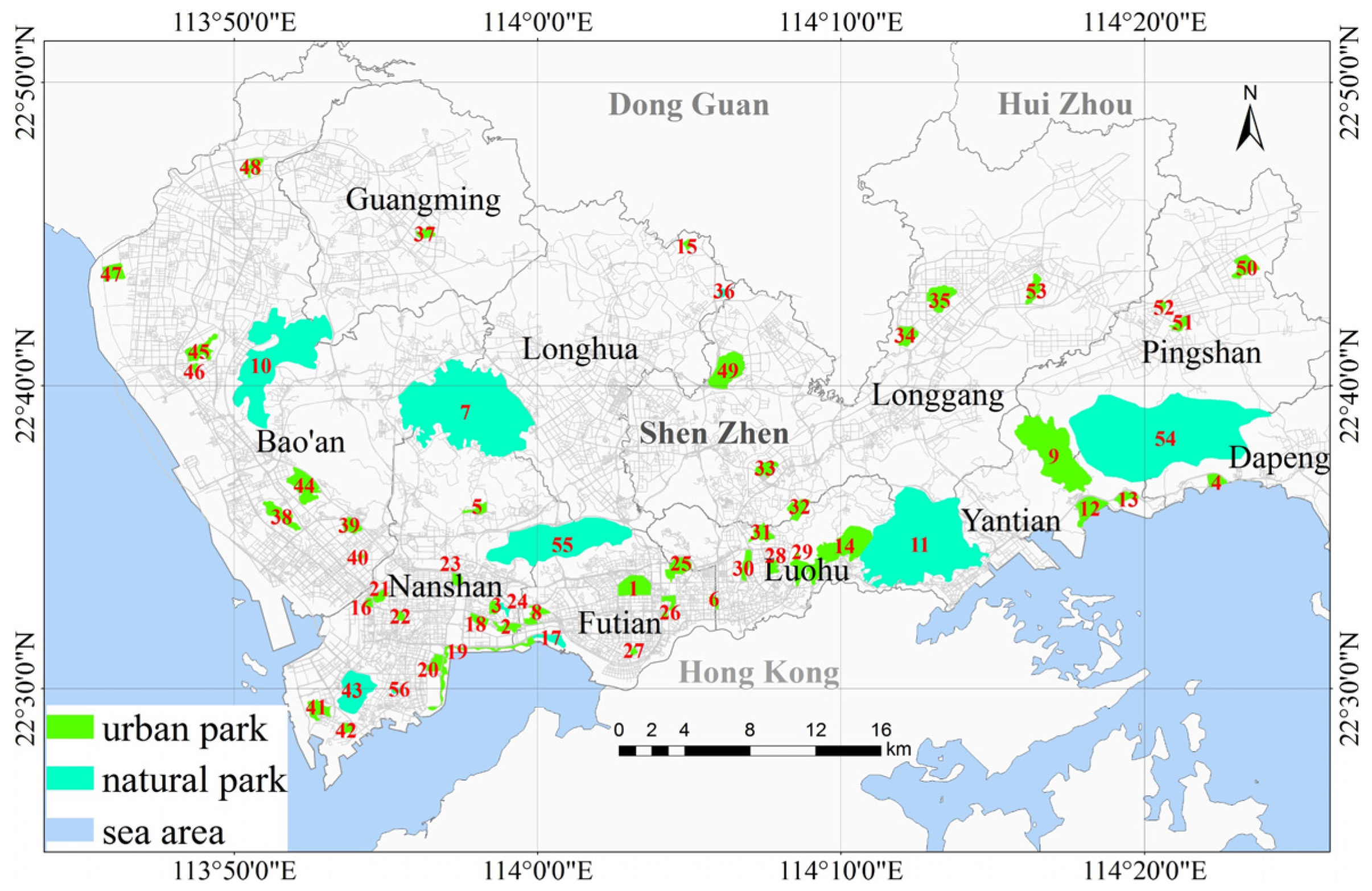
2. Study Area and Datasets
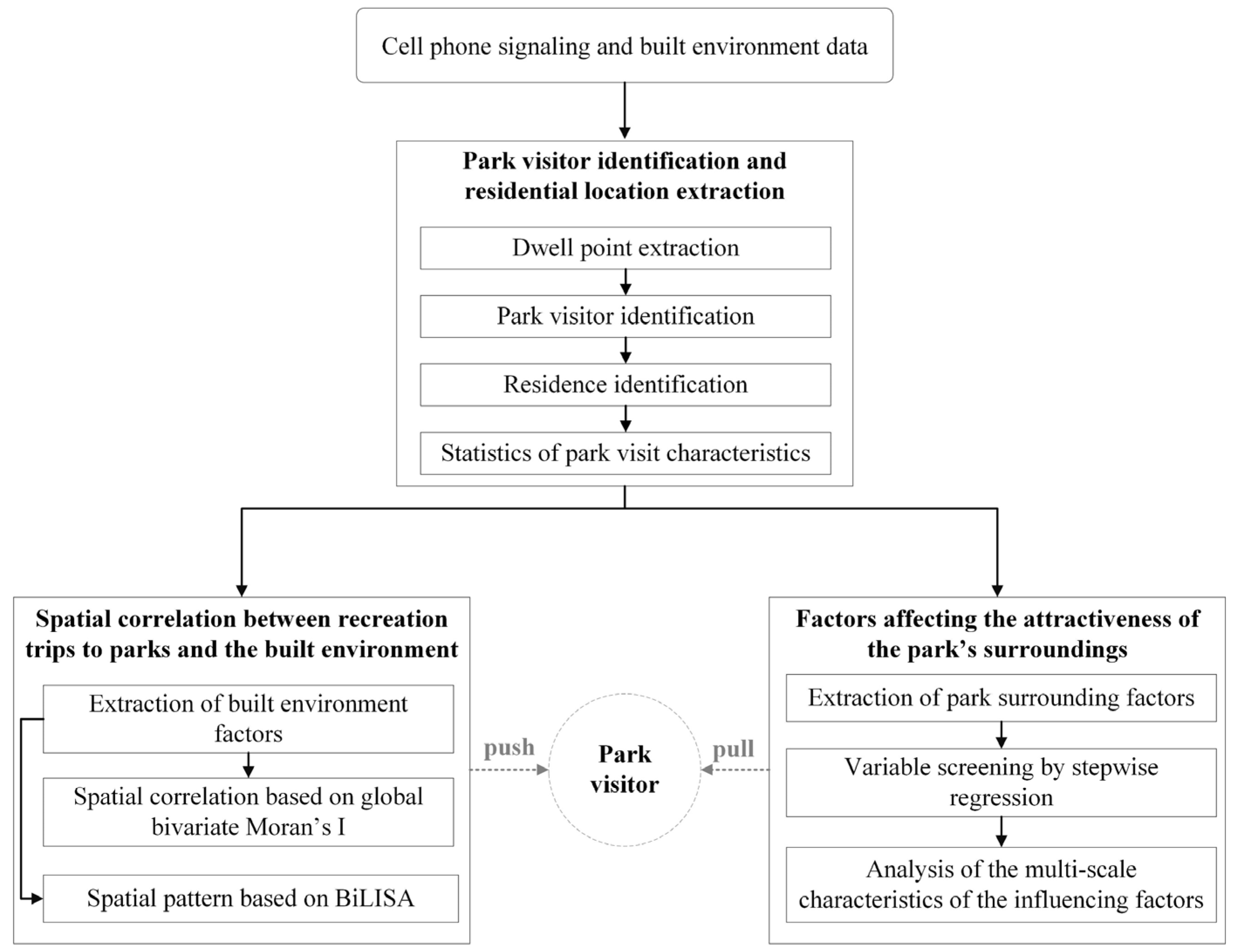
Shenzhen is located in the south of Guangdong, China, and is the core city of the Guangdong–Hong Kong–Macao Greater Bay Area. It is a city built in parks. From the five parks that were built at the beginning of the Reform and Opening-Up, this city has a total park area of 31,466.43 hectares today, with a coverage rate of 90.87% in a 500 m service radius. These parks constitute the natural ecosystem in Shenzhen. The park classification system of Shenzhen in 2020 divides them into three categories: urban parks, natural parks, and community parks [39]. Considering the positioning accuracy of the cell phone signal data used in this study, a total of 56 parks with a high matching degree between park size and the service coverage of the cell phone base station and which are known to residents were selected for this study (Figure 1, Appendix A Table A1). In the selected parks, the largest number belonged to urban parks, accounting for 48, whereas there were 9 nature parks. Community parks were not included in this study because of their small size.
To understand characteristics of the built environment that influence park recreation trips, the following data were used in this study: (1) Park data. We selected 56 large urban and natural parks and manually mapped the boundary of each park with the help of Gaode Maps and Google Images. (2) The cell phone signal data were processed indirectly by the API interface provided by China Mobile Communications Group Shenzhen Co., Ltd. This dataset contained activity records of all cell phones in the Shenzhen municipal area from 1 October 2019 to 31 October 2019. According to the statistical calculation method provided by China Mobile Communications Group, there were a total of 410 million cell phone records. (3) Point of interest (POI) data [41] were captured from the Gaode Maps open API interface [42] and converted to the WGS-84 coordinate system. There were 1.4 million records of POI data, covering 23 categories such as public facilities, companies, and businesses. The 23 categories were combined into 11 categories based on possible influences on park recreation trips, namely catering services (CS); corporate and enterprise services (CES); shopping services (SS); transportation facilities (TF); financial and insurance services (FIS); science, education, and culture services (SECS); residential housing (RH); living services (LS); sports and leisure services (SLS); health care services (HCS); and accommodation services (AS). (4) Electronic map and administrative boundary data. Road networks were downloaded from the Open Street Map website for 2019, and administrative boundary data from Resource and Environment Science and Data Center (RESDC) for 2015 [40] were used for mapping. (5) Vegetation condition data. Tree height data were obtained from the Global Land Analysis & Discovery group [43]. Vegetation index data (Landsat 8 enhanced vegetation index (EVI)) were downloaded from the Chinese Scientific Data [44] for the same time as the acquisition of cell phone signal data.

3. Methods

The research methodology of this paper is divided into three steps (as shown in Figure 2), as follows:
(1) Park visitor identification and residential location extraction
The cell phone signal data were processed through the API interface provided by China Mobile Communications Shenzhen. To protect the privacy of user data, the study area was divided into 22,693 grid cells of 250 m × 250 m, and the final aggregate results obtained through the API were used as the values of each grid cell.
First, we extracted the dwell points in the cell phone signaling data. A location where a resident exceeds the dwell time threshold (30 min) at a base station or multiple adjacent base stations during a trip was taken as a dwell point, and the latitude and longitude location of the dwell point was derived by the algorithm provided by China Mobile Communications Group Shenzhen Co., Ltd. Second, park visitors were extracted from the information provided by the dwell point data. The records that were not present in Shenzhen at night in one month were excluded to obtain the records of Shenzhen residents. Furthermore, records of park staff and short stays were removed to obtain results for all park visitors. Finally, we extracted the residences of park visitors and aggregated the visit characteristics of each park and the travel characteristics of each grid cell. In cities, parks are not always equitably distributed. Access to parkland is often based on age and gender, as well as other axes of difference. However, the criteria for classifying sociodemographic characteristics are not uniform for different research purposes. For example, Veitch [45] chose women aged 18–45 and children aged 5–12 to study differences in park characteristics between urban and rural areas, and Sister [17] used the number of children (aged under 17) as an index of park demand. Teenagers under the age of 18 have more opportunities to visit parks after school and on holidays, and older adults have more time to participate in park recreation after retirement in China. Therefore, we divided the park visitors into three groups in terms of availability of park recreation participation time (as shown in Table 1). The first group was males and females under the age of 18. In China, there is a difference in the retirement age between males and females, so here we used 55 years old for women and 60 years old for men as the retirement age threshold, and we also used this to divide adults into two groups, one for younger adults (Group 2) and the other for older adults (Group 3). We used the grid cell as the origin (O) of the recreation trips and the parks as the destination (D) of the trips. Finally, the average daily trips of the three groups for each O–D pair were counted during weekdays, weekends, and the National Day holiday. Moreover, we weighted the recreation trip distance of each grid cell to determine the service radius of each park. The service radius is calculated as follows:
D i = j n d i j x i j j n x i j
where D i is the service radius of the park i , d i j is the straight-line distance from the grid cell i to the park j , x i j is the number of recreation trips from the grid cell i to the park j , and n is the total number of grid cells that have visitors to the park i . In contrast to the service radius of a park specified at the time of planning, the service radius obtained by weighting the distance of the O–D pair actually represents the attractiveness of the park for the cell phone population. To further analyze the spatial aggregation of recreational trips in parks, we used Getis–Ord Gi* to generate spatial hotspot maps for different age groups in three time periods.
(2) Spatial correlation between recreation trips to parks and the built environment
The elements of the built environment that affect travel for park recreation activities are multidimensional and complex, involving land use, road systems, and services. Shenzhen is one of the most economically developed cities in China, with a small urban area and dense population, housing, and roads. At the same time, it is located in a subtropical region with lush vegetation in the city, making it a typical forest city. According to the density, diversity, and accessibility in the five dimensions of urban design [46], we divided the elements of the built environment into POI diversity, road density, population density, average building height, average tree height, and the mean value of EVI. According to the grid division of the study area, the values of each factor in each grid cell were calculated separately. In particular, POI diversity is represented by the entropy index, which is calculated as:
E I = S i × l n 1 S i
where E I is the entropy index of POI, i is the POI type, and S i is the proportion of class i POI in the grid out of the total number of POIs. The value of E I can reflect the mixing degree of city functions. The larger the entropy index is, the more balanced the distribution of various POIs in the city. On the contrary, the POI distribution tends to be regionally specialized.
On the basis of the above parameters, we used the global bivariate Moran’s I to explore the spatial correlation between park recreation trips and the built environment in each grid cell. The global bivariate Moran’s I statistic quantifies the spatial correlation between two variables x l and x k at the same location i and is defined as follows.
I k l = Z k W Z l n
where n is the number of observations, and Z k = x k x k ¯ / σ k and Z l = x l x l ¯ / σ l have been standardized such that the mean is 0 and the standard deviation equals 1. W is the row-standardized spatial weight matrix. The value of I k l is between −1 and 1. I k l > 0 means the variables are spatially positively correlated; the larger the value, the more obvious the spatial positive correlation. I k l < 0 means the variables are spatially negatively correlated; the smaller the value, the more obvious the spatial negative correlation. I k l = 0 means the variables are spatially randomly distributed.
The global bivariate Moran’s I does not provide any information on where the clusters exist. It is likely that the global statistics wrongly show that there is no relationship among the data, although there might be a strong correlation in different parts of the study area. The bivariate local Moran’s I (BiLISA) provides a measure of association for each grid cell and helps to identify the type of spatial correlation. The BiLISA can be defined as follows:
I k l i = Z k i j w i j Z l j
This statistic indicates the degree of linear association (positive or negative) between the value of one variable at a particular location i and the mean of another variable at a neighboring location (e.g., j s ). The result of BiLISA is a map representing the positive spatial cluster pattern (high–high or low–low cluster) and the negative spatial correlation or spatial outliers (high–low or low–high cluster) for the two variables, respectively. The global bivariate Moran’s I and BiLISA in this paper were conducted by GeoDa [47] software.
(3) Factors affecting the attractiveness of the park’s surroundings
The functional clustering and behavioral perceptions of a specific location [48] influence the activity patterns of residents, which are usually expressed as the recreational attractiveness of the park to residents, and are important criteria for measuring park quality. In addition to the park’s own facility elements, the type of services, road density, vegetation, and other features in its vicinity can also facilitate or constrain residents’ recreational activities and affect the duration of activities and the comfort of the experience. For this reason, we constructed multiple regression models using the average daily number of park visitors as the dependent variable and park environmental elements as the independent variables to measure the influence of each element on the number of park visitors. The parks’ environmental elements include three categories: the quality of the park’s vegetation, the richness of the surrounding facilities, and the road network density. The average tree height and EVI index are used to represent the ecological quality of the park. The road network density is used to represent the potential for travel to the park. The buffer zones of the park were set to 200, 400, 600, 800, and 1000 m, and the number of various POIs in the buffer zone is used to represent the richness of the surrounding facilities and to facilitate the subsequent exploration of the specific impact range of various facilities around parks. Finally, 58 variables were selected (as listed in Appendix A Table A2).
Multiple regression analysis was used to explore the correlation between elements of the surrounding environment and participation in recreational activities in large parks and to identify potential influencing factors and their magnitude. Stepwise regression analysis is a special form of multiple regression analysis. It is based on the principle of eliminating variables that do not have a significant effect on the dependent variable and introducing only those variables that have a significant effect on the dependent variable into the regression model, thus obtaining the best explanatory model. The general form of multiple regression analysis is
y = β 0 + β 1 x 1 + β 2 x 2 + + β m x m + ε
where y is the dependent variable, x i is the independent variable, β i is the correlation coefficient of the corresponding independent variable, and ε is the random error term in the regression model.

4. Results

4.1. Spatial and Temporal Characteristics of Park Visitation

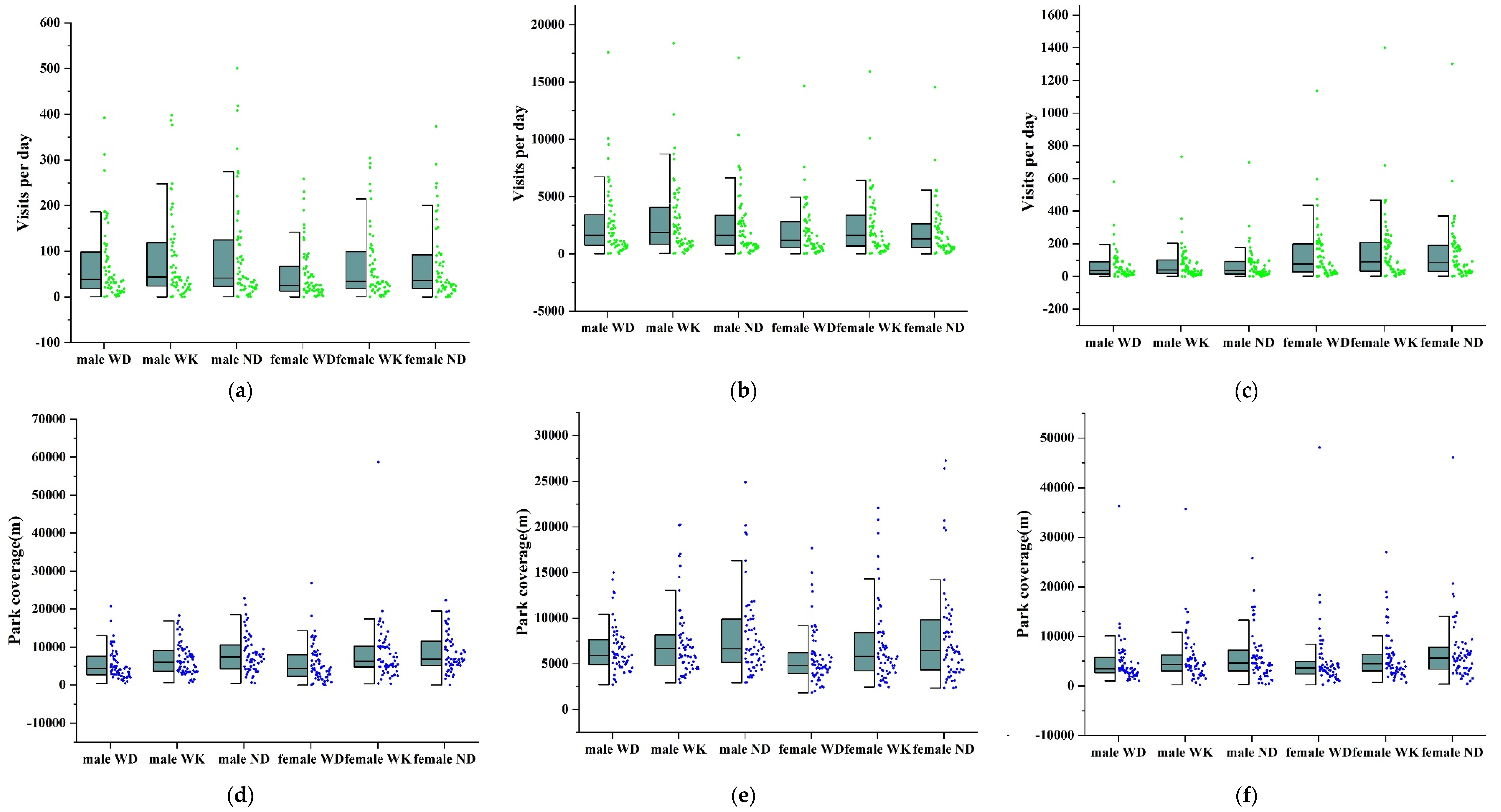
4.1.1. Characteristics of Recreation Trips to Parks

As can be seen in Table 1, this group had fewer park visits on weekdays and had the highest park visits on the National Day holiday. More males in this group participated in park recreation compared to females. In Group 2, there was a significant difference in the number of males and females visiting parks. In contrast to Group 1, weekends were the preferred recreation time for Group 2. In particular, the National Day holiday is a special time for travel and recreation activities in China, but surprisingly Group 2 made fewer recreation trips during this period than on weekdays. Group 3 is older adults. During the three time periods, almost twice as many elderly females as males visited. As can be summarized from Table 1, during the three time periods for which cell phone signal data were collected, teenagers made fewer recreation trips to parks, younger adults accounted for the largest proportion of recreation trips, and older females preferred park recreation activities compared to older males.
The spatial travel hotspots were quite similar for each time period and age group (as shown in Figure 3). The areas with higher park visits for each group in different time periods were mainly distributed in Futian; Luohu; the streets of Nanshan and Nantou in Nanshan District; and the streets of Xixiang, Xin’an, Fuhai, and Fuyong in Bao’an District. The difference was that the intensity of travel hotspots for Groups 1 and 3 in Nanshan and Bao’an districts changes at different times. Groups 2 and 3 were particularly scarce in travel hotspots in Longgang and Dapeng districts. Only Group 1 had obvious travel hotspots during weekends and the National Day in Longgang Street and Baolong Street. The major difference with Groups 1 and 3 was that Group 2 had obvious travel hotspots in Longhua Street and Bantian Street in all three time periods, whereas the other two groups were not obvious.

4.1.2. Efficiency of Park Services

Each point in Figure 4 represents the average daily visits and service radius for 56 parks in Shenzhen on weekdays, weekends, and the National Day holiday. To compare differences in the characteristics of park visits and park service radius (in persons/day, meters) across age groups and time periods, medians, which are not easily influenced by extreme values in the data, were used as the average daily visits. Figure 4a–c shows the daily park visits for the three age groups. The daily visits for males in Group 1 were the lowest (35.17) on weekdays, whereas the difference between the daily visits for weekends and the National Day holiday was not significant (41.12 and 40.5, respectively), and the order of daily visits for females was as follows: the National Day (35.76) > weekends (32.65) > weekdays (25.38). The order of daily visits of male visitors in Group 2 was as follows: the National Day (1455.5) > weekends (1408.58) > weekdays (1206.38). On weekdays and the National Day holiday, they outnumbered the females in the same group, whereas on weekends the two were closer (1353.56 for females). The daily visits for older males were lower than those for older females in the three time periods. In terms of the number of daily visits, Shenzhen’s parks were equally attractive to adolescent males and females, more attractive to males than females in Group 2, and less attractive to older males than older females in Group 3. Figure 4d–f shows the park service radius for the three age groups. The difference in park service radius between the weekdays and weekends was smaller for males and females in Group 1, and the difference between the service radius for males (7738.9) and females (6990.23) was larger on the National Day. Compared to Group 1, the park service radius for males and females in Group 2 differed significantly more between weekdays and weekends (6060.68 for males and 5196.85 for females on weekdays and 6813.27 for males and 6063.12 for females on weekends) and less on the National Day. In Group 3, the service radius for older males and females was similar to the characteristics in Group 1. Overall, the park service radius in the three groups at different time periods was in the order of weekdays < weekends < the National Day. The park service radius for males and females is the largest among the three time periods, and the shortest is weekdays.

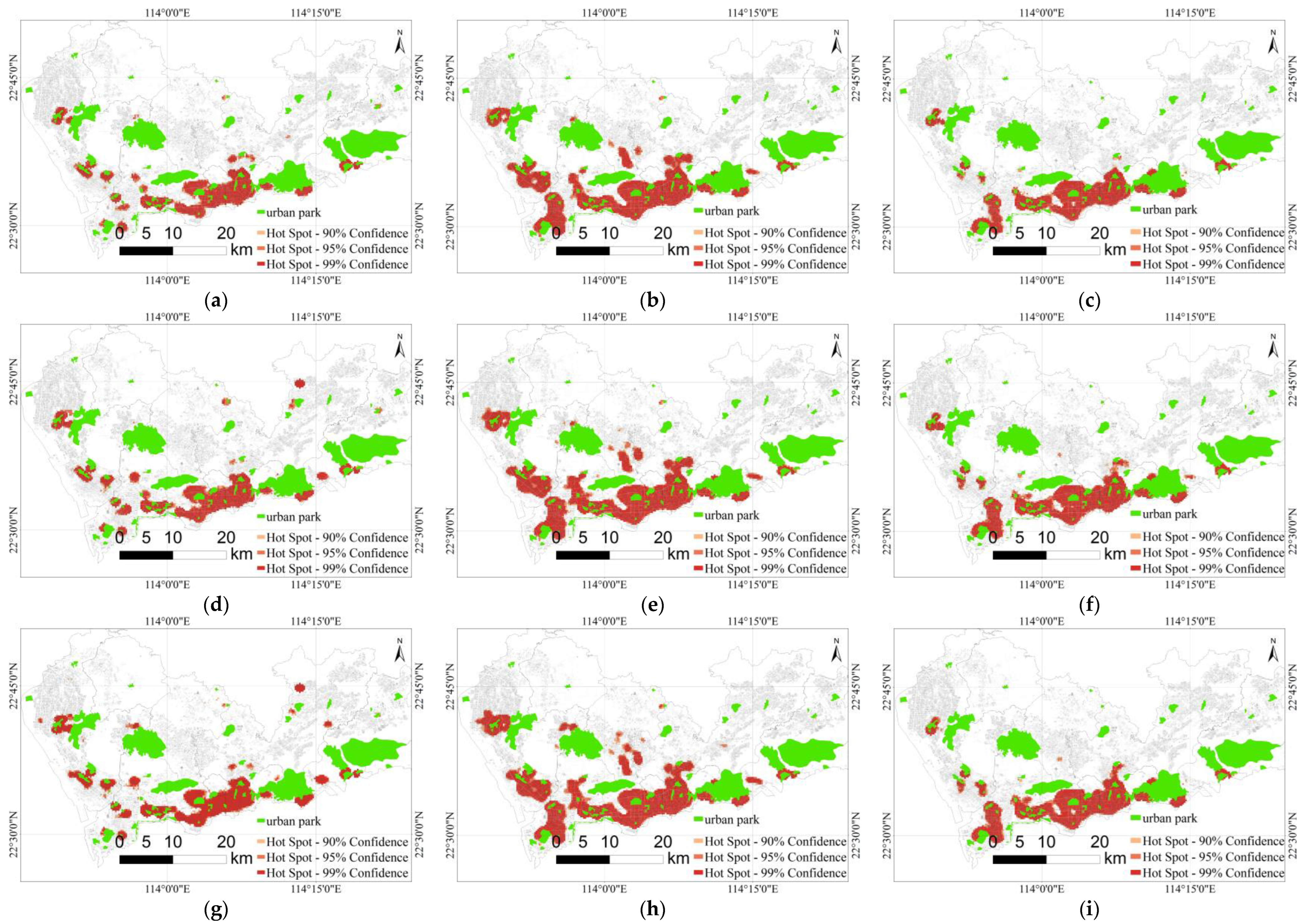
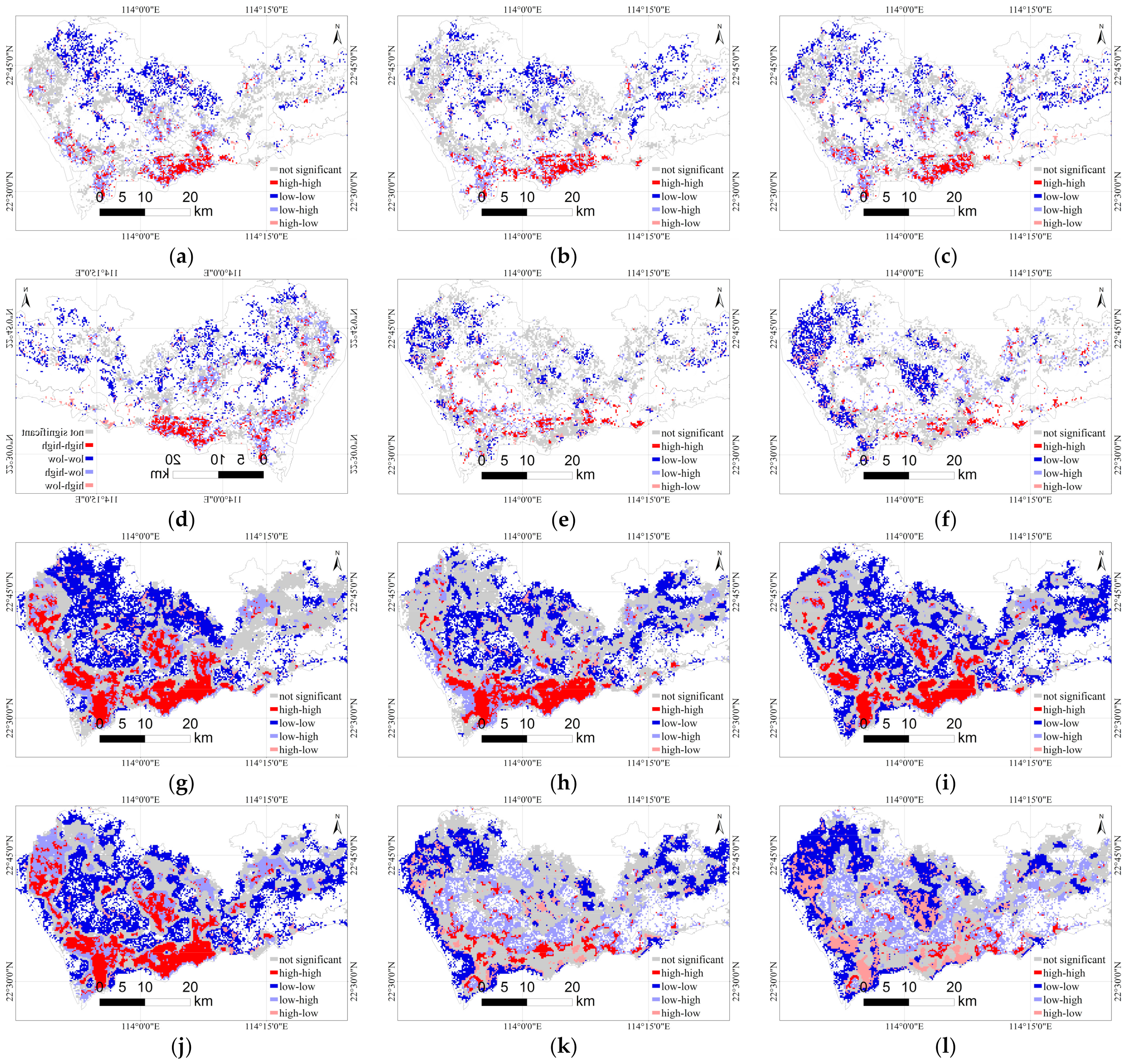
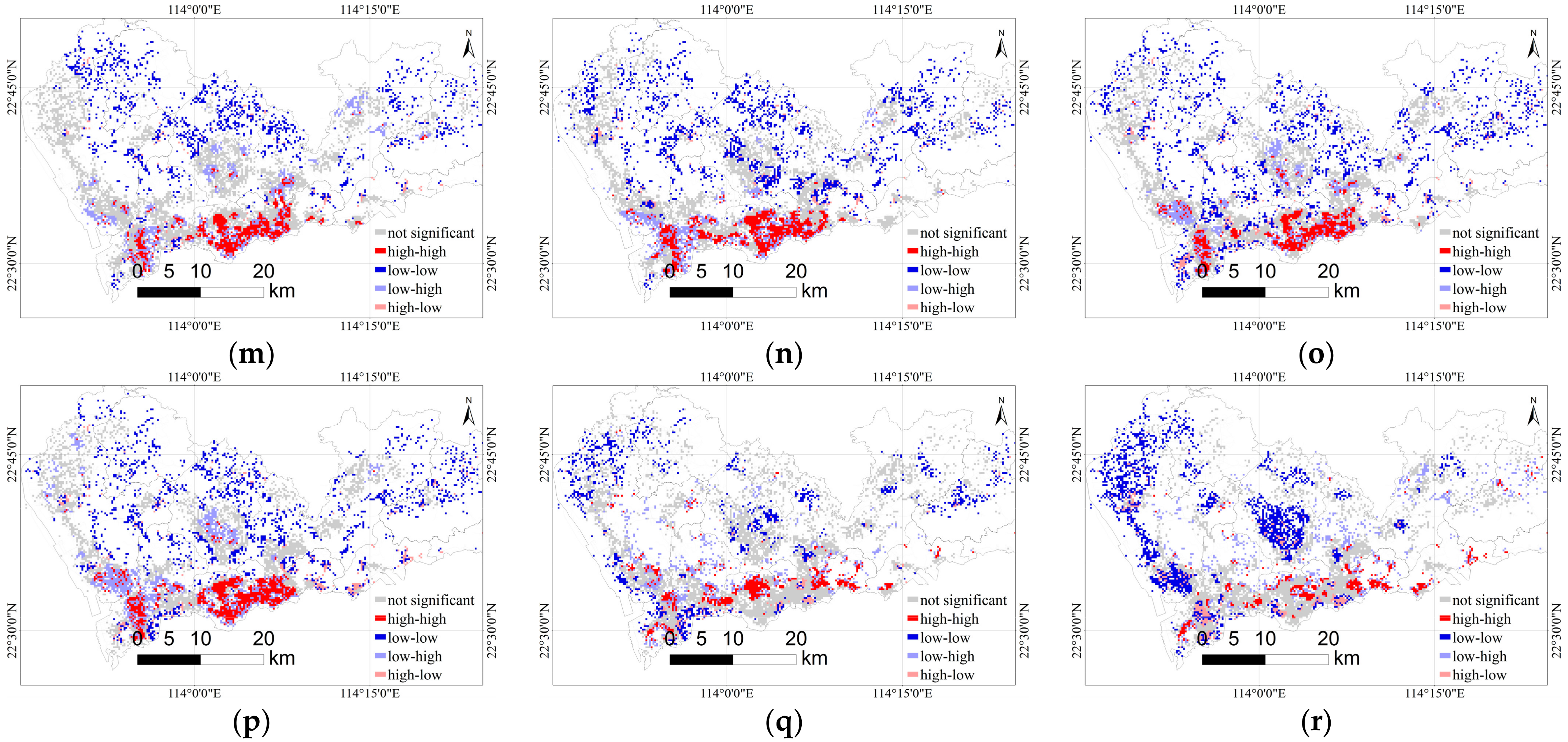
4.2. Spatial Correlation between Recreation Trips to Parks and the Built Environmental Factors

Table 2 shows the global bivariate Moran’s I (BMI) values between the average daily park recreation trips and the built environment elements for different age groups during weekdays, weekends, and the National Day. Overall, each variable showed a positive correlation with recreation trips to parks and passed the 0.001 significance level test, which indicated that the spatial correlation was obvious. In the 19–55/60 age range, the BMI values of male and female recreation trips with population density and POI diversity were greater than 0.25, indicating that this age range showed a significant correlation with these two variables. Meanwhile, they showed a significant correlation with the average height of buildings. Compared with other time periods, the BMI values in this age range with population density and POI diversity were the smallest during weekdays. The BMI values with EVI were smaller compared to all variables, with 0.025, 0.015, and 0.001 for weekdays, weekends, and the National Day, respectively. In the 7–18 age range, the correlations of recreation trips with each variable were lower and more varied for the three time periods; for example, the largest correlations were found for road density on weekdays and weekends, whereas the National Day has the largest correlation with POI diversity. This age range has an increasing correlation with each variable as the intensity of recreation trips increases; for example, the BMI values of POI diversity are in the order of weekdays (0.102) < weekends (0.113) < the National Day (0.120). In the >60/55 age range, recreation trips to parks for the three time periods reflected high correlations with road density and EVI, whereas they reflected lower correlations with the average height of buildings.
To further illustrate the spatial correlations between the number of recreation trips and built environment variables in each grid cell, three age-group spatial clustering maps were generated using BiLISA. From the results, the BiLISA spatial clustering maps were relatively similar for each age group in the three time periods. So here, we illustrated with the BiLISA spatial clustering map for the National Day (as shown in Figure 5). The red, light red, blue, and light blue in the figure indicate the high–high (I), high–low (II), low–low (III), and low–high (IV) spatial clustering characteristics of recreation trips with built environment variables, respectively. In southern Shenzhen, the three age groups showed high–high (I) patterns. These places are mainly located in areas with dense parks, buildings, and business activities, such as Futian and Nanshan districts. Groups 1 and 3 showed a sparser clustering pattern compared to Group 2. From Figure 5g–l, it can be seen that the recreational clustering with population density, POI diversity, and road network density of Group 2 showed a low–low (III) clustering pattern in northern and eastern Shenzhen, whereas a strong high–high (I) clustering pattern existed in southern Shenzhen. For the average height of buildings, there was a low–low clustering pattern in the north, a high–high clustering pattern in the south, and a less pronounced clustering pattern in the east. For the average tree height, the peripheral areas of Shenzhen showed a low–low clustering, the southern areas had fewer high–high values, and the central areas of Shenzhen had a clear low–high clustering. For the EVI index, its clustering characteristics showed a clear east–west variation. The low–low and high–low values are obviously clustered in the western part of Shenzhen, and the low–high and high–high values are obviously clustered in the eastern part of Shenzhen. In general, the spatial clustering characteristics of Group 1 and Group 3 are sparser (as shown in Figure 5a–f,m–r). Compared with Group 2, the high–high clustering was more obvious for the elderly in Group 3, whereas Group 2 showed more obvious low–low clustering, such as the average tree height and EVI in Figure 5a–f,m–r, with low–low values appearing denser in Group 1 in the east and high–high values appearing denser in Group 3 in the south.
Figure 6 shows a statistical heat map of the BiLISA results for recreation trips with each built environment variable for the three age groups. First, the number of grid cells in the high–high, low–low, low–high, and high–low patterns was calculated from the clustering maps, and their proportions in the total number of grid cells where recreation trips occurred were calculated. The horizontal coordinate in Figure 6 indicates the type of spatial clustering, the vertical coordinate indicates different time periods of the same variable, and the value indicates the proportion of grid cells in the spatial clustering pattern. As can be seen from the figure, the main difference between Groups 1 and 3 is that on weekends, the trips of the elderly are less correlated with the mean building height at high–high values, whereas the correlation increases at low–high and high–low values. The difference between Group 2 and Groups 1 and 3 is more obvious. The clustering characteristics related to the average building height, population density, POI diversity, and road network density are lower in Group 2 in the three time periods. Overall, the proportion of low–low clustering is larger in different groups, and the highest dependence on the average value of building height is evident in Group 2.

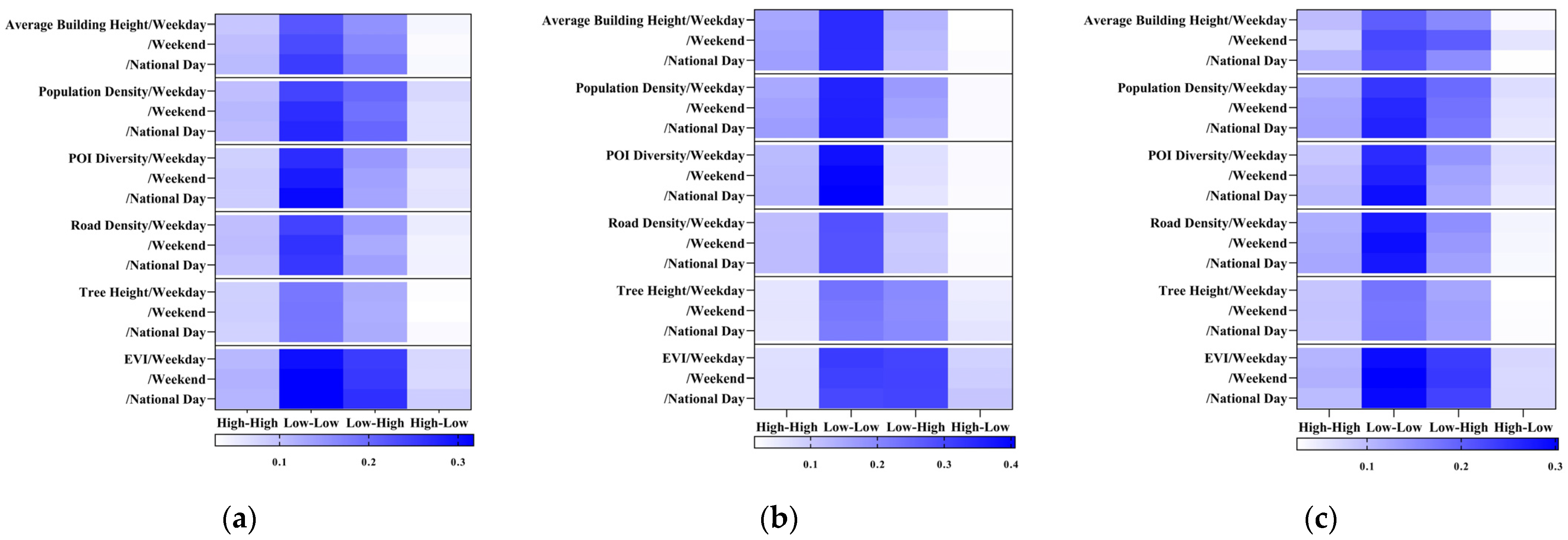
4.3. Factors Affecting the Attractiveness of the Park Surroundings

The 58 variables were screened by stepwise regression and the best models were found by the least squares method. Table 3 shows the 18 best models for different populations at the three time periods. The mean of the adjusted R-squared for all best models was 0.6998, which indicated the goodness of fit of the 18 models. The majority of models were fitted well except for females aged 7–18 on weekdays and weekends. Upon performing an F-test on the models, each regression model passed the 0.001 significance level. This indicated that the variables were effective in explaining the impact on the number of park visits.
In the 7–18 age group, the r2 values for males and females were lowest on weekends and highest on the National Day. The number of explanatory variables in the best model differed significantly across the three time periods. The number of explanatory variables for females was 5, 3, and 7 for weekdays, weekends, and the National Day holiday, respectively, whereas for males it was 3, 2, and 4, respectively. Especially on weekends, the type of explanatory variables in the model differed more than the other two periods. Group 2 had the best model fit on weekdays, with little difference in fit between weekends and the National Day holiday. Of the six models in Group 2, the difference in fit was greater for females aged 19–60 years on weekdays (r2 = 0.774) and weekends (r2 = 0.666). Group 3 had a good model fit on weekdays, weekends, and the National Day, and the number of explanatory variables in the model was relatively stable with four variables. Similar to the other two groups, the model had the highest fit value on weekdays.
In terms of the individual explanatory variables, transportation facilities (TF) appeared in 15 models. They only did not appear in the three models for weekdays and weekends for 7–18-year-olds. This indicates a significant positive correlation between TF and park visits, and the correlation is reflected in buffer distances of 200–400 m. The road density (RD) appeared in 14 models except for Group 1 and Group 2 on weekdays, and the positive regression weight value was followed only by TF. Moreover, the park visits were strongly correlated with RD at a park extent of 200 m. The total height of trees (THT) in the park was positively correlated with males on weekdays, whereas the correlations differed more at other times and for other age groups. In particular, THT did not appear in the model on weekends. EVI was more significantly positively correlated with each age group on weekends, whereas it differed more on weekdays and on the National Day. Particularly, EVI was negatively correlated with males aged 19–60 on weekdays. The range of EVI correlations was not consistent; for example, elderly and adult visits were positively correlated with EVI within 1000 m and 400 m of the park, respectively. SS was negatively correlated with park visits except for males aged 7–18 years on weekends, and the range of correlations was large (200–800 m). LS appeared only in the model for males aged 19–60 on weekdays and was negatively correlated. SLS did not appear in the six models of Group 3 and showed a positive correlation in the other groups except for Group 2 for females aged 19–55. Park area rarely appeared in the best model. SECS appeared in two models and showed a negative correlation. Additionally, FHCS and CS, although appearing in a small number, were positively correlated in several models.

5. Discussion

5.1. Park Visits Are Heterogeneous for Different User Groups

Although previous studies have investigated the role of the attributes of the built environment (e.g., density and diversity) in shaping the mobility of the general population (regardless of age) [49,50,51], they were based on the assumption that citizens most often use the nearest park [17]. As disposable income increases and transportation improves, urban residents can easily reach more distant parks for a variety of recreational activities [52]. Therefore, ignoring distant visitors may lead to an underestimation of actual park service capacity [53]. In addition, findings for the general population may not easily extend to population subgroups with many unique characteristics [54], such as younger and older adults. Our spatial correlation results suggested that average building height, road network density, and the diversity of points of interest were associated with high cluster characteristics for recreational trips to parks in residential areas. This result was more pronounced for adults (females aged 19–55 years, males aged 19–60 years). For younger and older adults, high–high clusters are more pronounced only in some areas, such as eastern Futian, whereas low–low clusters are more concentrated in the north. Evidence from previous studies on the relationship between individual recreational activities and the residential environment is limited and inconsistent. This may be due to the lack of fine-grained spatial and temporal data, as well as the lack of the subdivision of the population, resulting in (ignoring the heterogeneous usage patterns of different user groups) the inability to reveal the contribution of the built environment factors to recreational activities.
The service radius is commonly used to describe the park’s sphere of influence [55] and ability to serve visitors, with the radius being equal to the maximum desired distance for visitors to the park [56]. In practice, these are mostly determined by urban planners, and the designation of the park service radius, as well as its meaning, is not consistent across countries [53]. Two recent studies used big data methods to overcome the drawbacks of simply predetermining the service radius of parks [10,53]. The statistical results of the cell phone signal data showed that the service radius of urban parks in Beijing and Tianjin varied widely, ranging from 3 to 22 km. From our experimental results, the service radius of large parks in Shenzhen reflected by cell phone signals was above 5 km. We further confirmed that there were significant differences in the service radius of parks for different subpopulations at different time periods, and the service radius of parks for teenagers (Group 1) and older adults (Group 3) was smaller than that of younger adults (Group 2). Furthermore, the service radius of each subpopulation will increase with the availability of recreational travel opportunities. Our findings also further indicated that park planning should pay more attention to the spatially variable relationship of recreational trips to prevent possible imbalance in park allocation among subpopulations.

5.2. Human Activity and Remote Sensing Data Can Work Together to Explain the Attractiveness of the Park

In previous studies of park recreation impact factors, the types of factors of concern and the techniques used were diverse. These studies showed that the attractiveness of urban parks to visitors is the result of a combination of factors in the parks themselves and their surroundings [37,53]. It has also been confirmed that ecological infrastructure such as vegetation and water bodies in the park can reflect the attractiveness of the park [37,57]. However, manual survey methods for park vegetation are time-consuming and laborious. There was also a study that used Google Street View to measure the relationship between vegetation and mobility [54]. We, therefore, hypothesized that at the appropriate spatial scale, remote-sensing vegetation data may be an effective factor in characterizing the attractiveness of the park. This study combined EVI data and tree height data characterizing park ecology with POI data characterizing human activities and further confirmed that vegetation factors were reflected in the regression models for several population subgroups. This indicated that remote-sensing vegetation data can provide valid information for revealing park attractiveness factors. However, the explanatory power of different vegetation data varies greatly. Across the 18 models, the sum of tree heights appeared less frequently in the subpopulation groups than the sum of EVI. In addition, the sum of EVI was weaker in explaining the attractiveness in regression models for the older adults compared to teenagers and younger adults. Our observations support that ecology affects various populations to different degrees. One possible reason for this may be that high naturalness is important for young people and adults when assessing landscape values, but relatively unimportant among older adults [58].
Furthermore, the traditional approach to measuring park impacts is to delineate fixed buffers [10,38,53] at distances ranging from 200 to 1000 m. This approach makes it difficult to give a reasonable distance value and tends to ignore the heterogeneity of different impact factors. In this paper, we determined the spatial extent of each factor by using regression with buffer ranges of 200, 400, 600, 800, and 1000 m. The results revealed a disproportionate influence of distances for each factor in different population subgroups by comparing regression models. Policymakers and planners drafting park plans to improve public visitability should be aware of the effective distances of factors influencing park attractiveness.

5.3. Limitations and Future Research

In this paper, we took Shenzhen as an example and used cell phone signaling data as a basis for determining park visits. Compared with traditional park surveys and on-site statistics, cell phone signaling data can capture detailed information such as the departure location of park visitors. Moreover, this type of data also suffers from the problem of under-representation and can only be analyzed to derive the characteristics of park visitors who use cell phones. In addition, the localization error of cell phone signaling data depends on the strength of the associated localization algorithm. The data we used were provided by mobile communication companies with corrected positioning algorithms, which to a certain extent ensures the reliability of the data quality. Overall, the coverage and granularity of the data are still relatively high compared to traditional methods such as manual surveys and video monitoring. There are reliable records of where park visitors leave, when they visit, etc. Therefore, the obtained results have a high reliability in the population of cell phone users. In the future, we will continue to track park recreation activity studies with cell phone signal data and add data sources that can record park visitors, such as social networks. The reliability of the analysis of park visitors will be improved by this complementary long time series of observation data.

6. Conclusions

Parks play an important role in improving urban ecology and meeting the recreational needs of citizens. Therefore, exploring the spatiotemporal characteristics of park visitors and the “push–pull” factors that shape this mobility is critical for designing and managing urban parks. First, information on park visitors’ departure locations and the visited parks was extracted using cell phone signal data to explore the differential characteristics of recreation trips to parks for different groups of people. Second, the association between recreation trips to parks and the urban built environment was examined with the help of global bivariate Moran’s I and BiLISA using satellite vegetation, building height, and POI data. Finally, we developed multiple regression models with the number of park visits as the dependent variable to quantify the constituent factors affecting park attractiveness. Our study showed the following: (1) Recreation visitors at large parks varied significantly among population subgroups. Compared with younger adults, teenagers and older adults traveled smaller distances and made fewer trips, and in particular, older adults of different genders differed significantly in park participation. (2) Recreational trips in large parks were related to the functional layout of the built environment around their residence. In areas with rich urban functions (e.g., southern Shenzhen), trips to large parks for recreation are more aggregated. (3) The findings reinforce the evidence that remote sensing data of urban vegetation can be an effective factor in characterizing park attractiveness, but the explanatory power of different vegetation data varies widely. Therefore, we suggest that park planning should pay more attention to the spatially changing characteristics of recreation trips to prevent the imbalance on the park configuration for potential subpopulations and integrate complementary human activity and remote sensing data to ensure real-time and reliable urban park recreation research and planning to adapt to changing urbanization trends.

Author Contributions

Conceptualization, methodology, validation, formal analysis, writing—original draft preparation, B.H., K.L.; resources, data curation, K.L., B.H.; review and editing, J.F., J.H.; funding acquisition, project administration, B.H., K.L.; investigation, validation, visualization, B.H., L.N., J.X. All authors have read and agreed to the published version of the manuscript.

Funding

This research was funded by the National Key Research and Development Project of China (No. 2019YFB2102500), the National Natural Science Foundation of China (No. 41901391), and the Shenzhen Fundamental Research Program (No. JCYJ20190812171419161, JCYJ20190807163001783).

Data Availability Statement

The Gaode POI data are available from https://lbs.amap.com/api/webservice/guide/api/search (accessed on 23 December 2021). The administrative boundary data are available from https://www.resdc.cn/ (accessed on 23 December 2021). The tree height data are available from https://glad.umd.edu/dataset/gedi/ (accessed on 23 December 2021). The Landsat 8 enhanced vegetation index data are available from http://databank.casearth.cn (accessed on 23 December 2021).

Conflicts of Interest

The authors declare no conflict of interest.

Appendix A

Table A1. List of selected parks in Shenzhen.
IDNameIDName
1Lianhua Mountain Park30Honghu Park
2Jinxiuzhonghua Folk Village31Weiling Park
3Happy Valley32Qiushuishan Park
4Rose Coast33Shiyaling Xinyi Sports Park
5Shenzhen Wild Animal Park34Dayun Park
6Lizhi Park35Longcheng Park
7Yangtaishan Forest Park36Guanlan Shanshui Tian Yuan Tourism and Culture Park
8International Garden and Flower Expo37Guangming New Town Park
9Eastern Overseas Chinese Town38Tiezai Mountain Park
10Fenghuangshan Forest Park39Baoan Park
11Wutong Mountain40Lingzhi Park
12Dameisha41Xiaonanshan Park
13Xiaomesha42Wen Tianxiang Memorial Park
14Xianhu Botanical Garden43Nanshan Park
15Guanlan Printmaking Village44Pinglun Mountain Park
16Dutch Flower Town45Lixin Lake Park
17Mangrove Nature Reserve46Wangniuting Park
18Window of the World47Sea Field Park
19Shenzhen Bay Park48Qilin Mountain Park
20Talent Park49Pinghu Ecological Park
21Zhongshan Park50Julongsan Ecological Park
22Lixiang Park51Yanziling Ecological Park
23Dashahe Park52Pingshan Central Park
24Yanhanshan Country Park53Baxianling Park
25Bijia Mountain Park54Malushan Country Park
26Shenzhen Central Park55Tanglang Mountain Park
27Huanggang Park56Sihai Park
28Cuizhu Park
29Donghu Park
Table A2. The variables for analyzing the attractiveness of the park’s surroundings.
AREATFRDTree HeightEVISSLSSLSSECSHCSCSAS
MeanSumMeanSum
No buffer
200 m
400 m
600 m
800 m
1000 m
Note: √ indicates the selected variable. The abbreviations in the table are as follows: park area (AREA); transportation facilities (TF); road density (RD); enhanced vegetation index (EVI); shopping services (SS); living services (LS); sports and leisure services (SLS); science, education, and culture services (SECS); health care services (HCS); catering services (CS); and accommodation services (AS).

References

  1. Wang, J.; Wang, J.; Foley, K. Assessing the performance of urban open space for achieving sustainable and resilient cities: A pilot study of two urban parks in Dublin, Ireland. Urban For. Urban Green. 2021, 62, 127180. [Google Scholar] [CrossRef]
  2. Tian, M.; Yuan, L.; Guo, R.; Wu, Y.; Liu, X. Sustainable development: Investigating the correlations between park equality and mortality by multilevel model in Shenzhen, China. Sustain. Cities Soc. 2021, 75, 103385. [Google Scholar] [CrossRef]
  3. Liu, Y.; Zhang, Y.; Jin, S.T.; Liu, Y. Spatial pattern of leisure activities among residents in Beijing, China: Exploring the impacts of urban environment. Sustain. Cities Soc. 2020, 52, 101806. [Google Scholar] [CrossRef]
  4. Rigolon, A.; Browning, M.; Jennings, V. Inequities in the quality of urban park systems: An environmental justice investigation of cities in the United States. Landsc. Urban Plan. 2018, 178, 156–169. [Google Scholar] [CrossRef]
  5. Song, Y.; Huang, B.; Cai, J.; Chen, B. Dynamic assessments of population exposure to urban greenspace using multi-source big data. Sci. Total Environ. 2018, 634, 1315–1325. [Google Scholar] [CrossRef] [PubMed]
  6. Kaczynski, A.T.; Potwarka, L.R.; Saelens, B.E. Association of Park Size, Distance, and Features with Physical Activity in Neighborhood Parks. Am. J. Public Health 2008, 98, 1451–1456. [Google Scholar] [CrossRef] [PubMed]
  7. Cohen, D.A.; Marsh, T.; Williamson, S.; Derose, K.P.; Martinez, H.; Setodji, C.; McKenzie, T.L. Parks and physical activity: Why are some parks used more than others? Prev. Med. 2010, 50 (Suppl. S), S9–S12. [Google Scholar] [CrossRef] [PubMed] [Green Version]
  8. Giles-Corti, B.; Broomhall, M.H.; Knuiman, M.; Collins, C.; Douglas, K.; Ng, K.; Lange, A.; Donovan, R.J. Increasing walking: How important is distance to, attractiveness, and size of public open space? Am. J. Prev. Med. 2005, 28, 169–176. [Google Scholar] [CrossRef]
  9. Ministry of Housing and Urban-Rural Development of the People’s Republic of China. Standard for Classification of Urban Green Space; China Architecture Publishing & Media Co, Ltd.: Beijing, China, 2017.
  10. Guo, S.; Yang, G.; Pei, T.; Ma, T.; Song, C.; Shu, H.; Du, Y.; Zhou, C. Analysis of factors affecting urban park service area in Beijing: Perspectives from multi-source geographic data. Landsc. Urban Plan. 2019, 181, 103–117. [Google Scholar] [CrossRef]
  11. Veitch, J.; Bagley, S.; Ball, K.; Salmon, J. Where do children usually play? A qualitative study of parents’ perceptions of influences on children’s active free-play. Health Place 2006, 12, 383–393. [Google Scholar] [CrossRef] [Green Version]
  12. Bertram, C.; Meyerhoff, J.; Rehdanz, K.; Wüstemann, H. Differences in the recreational value of urban parks between weekdays and weekends: A discrete choice analysis. Landsc. Urban Plan. 2017, 159, 5–14. [Google Scholar] [CrossRef]
  13. Czerniak, J.; Hargreaves, G.; Beardsley, J. Large Parks; Princeton Architectural Press: New York, NY, USA, 2007. [Google Scholar]
  14. Xing, L.; Liu, Y.; Liu, X. Measuring spatial disparity in accessibility with a multi-mode method based on park green spaces classification in Wuhan, China. Appl. Geogr. 2018, 94, 251–261. [Google Scholar] [CrossRef]
  15. Lin, Y.; Zhou, Y.; Lin, M.; Wu, S.; Li, B. Exploring the disparities in park accessibility through mobile phone data: Evidence from Fuzhou of China. J. Environ. Manag. 2021, 281, 111849. [Google Scholar] [CrossRef]
  16. Liu, B.; Tian, Y.; Guo, M.; Tran, D.; Alwah, A.A.Q.; Xu, D. Evaluating the disparity between supply and demand of park green space using a multi-dimensional spatial equity evaluation framework. Cities 2022, 121, 103484. [Google Scholar] [CrossRef]
  17. Sister, C.; Wolch, J.; Wilson, J. Got green? addressing environmental justice in park provision. GeoJournal 2010, 75, 229–248. [Google Scholar] [CrossRef]
  18. Maroko, A.R.; Maantay, J.A.; Sohler, L.N.; Grady, K.L.; Arno, P.S. The complexities of measuring access to parks and physical activity sites in New York City: A quantitative and qualitative approach. Int. J. Health Geogr. 2009, 8, 34. [Google Scholar] [CrossRef] [Green Version]
  19. Wolch, J.R.; Byrne, J.A.; Newell, J.P. Urban green space, public health, and environmental justice: The challenge of making cities ‘just green enough’. Landsc. Urban Plan. 2014, 125, 234–244. [Google Scholar] [CrossRef] [Green Version]
  20. Guo, S.; Song, C.; Pei, T.; Liu, Y.; Ma, T.; Du, Y.; Chen, J.; Fan, Z.; Tang, X.; Peng, Y.; et al. Accessibility to urban parks for elderly residents: Perspectives from mobile phone data. Landsc. Urban Plan. 2019, 191, 103642. [Google Scholar] [CrossRef]
  21. Knapp, M.; Gustat, J.; Darensbourg, R.; Myers, L.; Johnson, C. The Relationships between Park Quality, Park Usage, and Levels of Physical Activity in Low-Income, African American Neighborhoods. Int. J. Environ. Res. Public Health 2018, 16, 85. [Google Scholar] [CrossRef] [PubMed] [Green Version]
  22. Zhang, S.; Zhou, W. Recreational visits to urban parks and factors affecting park visits: Evidence from geotagged social media data. Landsc. Urban Plan. 2018, 180, 27–35. [Google Scholar] [CrossRef]
  23. Cheng, L.; Chen, X.; Yang, S.; Cao, Z.; De Vos, J.; Witlox, F. Active travel for active ageing in China: The role of built environment. J. Transp. Geogr. 2019, 76, 142–152. [Google Scholar] [CrossRef]
  24. Lee, K.H.; Schuett, M.A. Exploring spatial variations in the relationships between residents’ recreation demand and associated factors: A case study in Texas. Appl. Geogr. 2014, 53, 213–222. [Google Scholar] [CrossRef]
  25. Donahue, M.L.; Keeler, B.L.; Wood, S.A.; Fisher, D.M.; Hamstead, Z.A.; McPhearson, T. Using social media to understand drivers of urban park visitation in the Twin Cities, MN. Landsc. Urban Plan. 2018, 175, 1–10. [Google Scholar] [CrossRef]
  26. Liu, H.; Li, F.; Xu, L.; Han, B. The impact of socio-demographic, environmental, and individual factors on urban park visitation in Beijing, China. J. Clean. Prod. 2017, 163, S181–S188. [Google Scholar] [CrossRef]
  27. Irvine, K.N.; Warber, S.L.; Devine-Wright, P.; Gaston, K.J. Understanding Urban Green Space as a Health Resource: A Qualitative Comparison of Visit Motivation and Derived Effects among Park Users in Sheffield, UK. Int. J. Environ. Res. Public Health 2013, 10, 417–442. [Google Scholar] [CrossRef]
  28. Zhang, H.; Chen, B.; Sun, Z.; Bao, Z. Landscape perception and recreation needs in urban green space in Fuyang, Hangzhou, China. Urban For. Urban Green. 2013, 12, 44–52. [Google Scholar] [CrossRef]
  29. Zhang, W.; Yang, J.; Ma, L.; Huang, C. Factors affecting the use of urban green spaces for physical activities: Views of young urban residents in Beijing. Urban For. Urban Green. 2015, 14, 851–857. [Google Scholar] [CrossRef]
  30. Martí, P.; Serrano-Estrada, L.; Nolasco-Cirugeda, A. Using locative social media and urban cartographies to identify and locate successful urban plazas. Cities 2017, 64, 66–78. [Google Scholar] [CrossRef]
  31. Hamstead, Z.A.; Fisher, D.; Ilieva, R.T.; Wood, S.A.; McPhearson, T.; Kremer, P. Geolocated social media as a rapid indicator of park visitation and equitable park access. Comput. Environ. Urban Syst. 2018, 72, 38–50. [Google Scholar] [CrossRef]
  32. Liu, H.; Li, F.; Li, J.; Zhang, Y. The relationships between urban parks, residents’ physical activity, and mental health benefits: A case study from Beijing, China. J. Environ. Manag. 2017, 190, 223–230. [Google Scholar] [CrossRef]
  33. García-Palomares, J.C.; Gutiérrez, J.; Mínguez, C. Identification of tourist hot spots based on social networks: A comparative analysis of European metropolises using photo-sharing services and GIS. Appl. Geogr. 2015, 63, 408–417. [Google Scholar] [CrossRef]
  34. Li, F.; Li, F.; Li, S.; Long, Y. Deciphering the recreational use of urban parks: Experiments using multi-source big data for all Chinese cities. Sci. Total Environ. 2020, 701, 134896. [Google Scholar] [CrossRef] [PubMed]
  35. Liu, Q.; Ullah, H.; Wan, W.; Peng, Z.; Hou, L.; Qu, T.; Haidery, S.A. Analysis of Green Spaces by Utilizing Big Data to Support Smart Cities and Environment: A Case Study About the City Center of Shanghai. ISPRS Int. J. Geo-Inf. 2020, 9, 360. [Google Scholar] [CrossRef]
  36. Liu, Q.; Ullah, H.; Wan, W.; Peng, Z.; Muzahid, A.A.M. Categorization of green spaces for a sustainable environment and smart city architecture by utilizing big data. Electronics 2020, 9, 1028. [Google Scholar] [CrossRef]
  37. Ćwik, A.; Kasprzyk, I.; Wójcik, T.; Borycka, K.; Cariñanos, P. Attractiveness of urban parks for visitors versus their potential allergenic hazard: A case study in Rzeszów, Poland. Urban For. Urban Green. 2018, 35, 221–229. [Google Scholar] [CrossRef]
  38. Wu, L.; Kim, S.K. Health outcomes of urban green space in China: Evidence from Beijing. Sustain. Cities Soc. 2021, 65, 102604. [Google Scholar] [CrossRef]
  39. Urban Administration and Law Enforcement Bureau of Shenzhen Municipality. Available online: http://cgj.sz.gov.cn/xsmh/szgy/index.html (accessed on 23 December 2021).
  40. Resource and Environment Science and Data Center (RESDC), Chinese Academy of Sciences. Available online: http://www.resdc.cn (accessed on 23 December 2021).
  41. Liu, K.; Yin, L.; Lu, F.; Mou, N. Visualizing and exploring POI configurations of urban regions on POI-type semantic space. Cities 2020, 99, 102610. [Google Scholar] [CrossRef]
  42. Gaode Map Open API Interface. Available online: https://lbs.amap.com/api/webservice/guide/api/search (accessed on 23 December 2021).
  43. Global Forest Canopy Height Data. Available online: https://glad.umd.edu/dataset/gedi/ (accessed on 23 December 2021).
  44. Landsat Spectral Indices Products over China. Available online: http://databank.casearth.cn (accessed on 23 December 2021).
  45. Veitch, J.; Salmon, J.; Ball, K.; Crawford, D.; Timperio, A. Do features of public open spaces vary between urban and rural areas? Prev. Med. 2013, 56, 107–111. [Google Scholar] [CrossRef] [Green Version]
  46. Ewing, R.; Cervero, R. Travel and the Built Environment: A meta-analysis. J. Am. Plan. Assoc. 2010, 76, 265–294. [Google Scholar] [CrossRef]
  47. GeoDa. Available online: http://geodacenter.github.io/index.html (accessed on 23 December 2021).
  48. Lee, G.; Hong, I. Measuring spatial accessibility in the context of spatial disparity between demand and supply of urban park service. Landsc. Urban Plan. 2013, 119, 85–90. [Google Scholar] [CrossRef]
  49. Alfonzo, M.; Guo, Z.; Lin, L.; Day, K. Walking, obesity and urban design in Chinese neighborhoods. Prev. Med. 2014, 69, S79–S85. [Google Scholar] [CrossRef]
  50. Pan, H.; Shen, Q.; Zhang, M. Influence of Urban form on Travel Behaviour in Four Neighbourhoods of Shanghai. Urban Stud. 2009, 46, 275–294. [Google Scholar] [CrossRef]
  51. Wei, X.; Huang, S.; Stodolska, M.; Yu, Y. Leisure Time, Leisure Activities, and Happiness in China: Evidence from a national survey. J. Leis. Res. 2015, 47, 556–576. [Google Scholar] [CrossRef]
  52. Yin, X. New Trends of Leisure Consumption in China. J. Fam. Econ. Issues 2005, 26, 175–182. [Google Scholar] [CrossRef]
  53. Li, F.; Yao, N.; Liu, D.; Liu, W.; Sun, Y.; Cheng, W.; Li, X.; Wang, X.; Zhao, Y. Explore the recreational service of large urban parks and its influential factors in city clusters—Experiments from 11 cities in the Beijing-Tianjin-Hebei region. J. Clean. Prod. 2021, 314, 128261. [Google Scholar] [CrossRef]
  54. Yang, L.; Liu, J.; Lu, Y.; Ao, Y.; Guo, Y.; Huang, W.; Zhao, R.; Wang, R. Global and local associations between urban greenery and travel propensity of older adults in Hong Kong. Sustain. Cities Soc. 2020, 63, 102442. [Google Scholar] [CrossRef]
  55. Lancaster, R.A. Recreation, Park and Open Space Standards and Guidelines; National Recreation and Park Association: Ashburn, VA, USA, 1983; pp. 141–168. [Google Scholar]
  56. Nicholls, S. Measuring the accessibility and equity of public parks: A case study using GIS. Manag. Leis. 2001, 6, 201–219. [Google Scholar] [CrossRef]
  57. Dade, M.C.; Mitchell, M.G.E.; Brown, G.; Rhodes, J.R. The effects of urban greenspace characteristics and socio-demographics vary among cultural ecosystem services. Urban For. Urban Green. 2020, 49, 126641. [Google Scholar] [CrossRef]
  58. Zube, E.H.; Pitt, D.G.; Evans, G.W. A lifespan developmental study of landscape assessment. J. Environ. Psychol. 1983, 3, 115–128. [Google Scholar] [CrossRef]
Figure 1. Distribution of parks in the study area. The numbers represent the selected parks listed in Table 1. City boundary data are from RESDC [40]. For clarity, Dapeng District is not fully included in the map.
Remotesensing 14 00499 g001
Figure 2. The research methodology and flow chart of data analysis.
Remotesensing 14 00499 g002
Figure 3. Distribution of the travel hotspots of the three groups on weekdays, weekends, and the National Day holiday. (ac) Travel hotspots of Group 1, Group 2, and Group 3 on weekdays; (df) Travel hotspots of Group 1, Group 2, and Group 3 on weekends; (gi) Travel hotspots of Group 1, Group 2, and Group 3 on the National Day holiday.
Remotesensing 14 00499 g003
Figure 4. The average daily visits and service radius of different groups in 56 parks on weekdays (WD), weekends (WK), and the National Day holiday (ND). (ac) Number of daily park visits for Groups 1, 2, and 3. (df) Park service radius for Groups 1, 2, and 3.
Remotesensing 14 00499 g004
Figure 5. The BiLISA spatial clustering maps of recreation trips to parks with built environment variables. (af) Spatial clustering characteristics of Group 1 with the average building height, road density, POI diversity, population density, average tree height, and the mean value of EVI. (gl) Spatial clustering characteristics of Group 2. (mr) Spatial clustering characteristics of Group 3.
Remotesensing 14 00499 g005aRemotesensing 14 00499 g005b
Figure 6. The statistical heat map of the BiLISA results. (a) Statistical heat map of the BiLISA results for Group 1. (b) Statistical heat map of the BiLISA results for Group 2. (c) Statistical heat map of the BiLISA results for Group 3.
Remotesensing 14 00499 g006
Table 1. Average number of daily trips in three time periods for different age groups (persons/day).
GroupGenderAgeWorkdayWeekendNational Day
Group 1 (teenagers)Male7–18437952245688
Female7–18326342224434
Group 2 (younger adults)Male19–60163,334182,741159,278
Female19–55122,416146,228125,185
Group 3 (older adults)Male>60413647824375
Female>55864299798830
Table 2. The BMI values between recreation trips to parks and the built environment factors.
Time PeriodAge GroupAge RangeAverage Building HeightRoad DensityAverage Tree Height EVI MeanPopulation DensityPOI Diversity
WorkdayGroup 17–180.0890.1130.0660.1110.0720.102
Group 219–55/600.2060.1840.036−0.0330.2640.281
Group 3>60/550.0750.1150.0920.1330.0890.08
WeekendGroup 17–180.0980.1290.0670.1090.0900.113
Group 219–55/600.2250.1970.033−0.0520.2940.304
Group 3>60/550.0820.1340.1000.1280.1160.105
National DayGroup 17–180.1050.1130.0680.1000.0880.120
Group 219–55/600.2290.1950.025−0.0700.3040.311
Group 3>60/550.0970.1350.0980.1290.1300.125
Table 3. The best regression model for each age and gender group.
WorkdayWeekendNational Day
Group123123123
Sex/AgeMale 7–18Female 7–18Male 19–60Female 19–55Male >60Female >55Male 7–18Female 7–18Male 19–60Female 19–55Male >60Female >55Male 7–18Female 7–18Male 19–60Female 19–55Male > 60Female > 55
Adj R 2 0.7100.6150.7600.7370.7700.7990.6690.5870.6550.6610.7230.7190.7520.6630.6760.6600.7230.718
R 2 0.7330.6400.7740.7540.7850.8120.6850.6000.6660.6820.7410.7370.7790.6850.6910.6860.7400.736
CS 0.676   5 /////////// 0.748   5 /////
HCS///////// 0.174   1 ////////
SECS 0.739   5 /////////// 0.887   5 /////
AREA// 0.563 ////////// 0.423 0.337 ///
SLS/ 0.958   3 / 0.476   5 // 0.455   2 0.676   2 //// 0.235   1 0.428   1 / 0.188   2 //
LS//// 0.214   2 0.212   2 ////////////
SS/// 0.161   4 // 0.458   1 0.170   5 0.245   3 0.234   3 0.371   3 // 0.272   4 0.278   3 0.276   3
EVI// 0.293   1 / 0.232   5 / 0.514   2 0.517   2 0.392   2 0.345   2 0.210   5 0.199   5 //// 0.191   5 0.186   5
THT 0.293 0.368 / 0.234 / 0.196 ////// 0.351 // 0.250 //
RD 0.504   1 0.717   1 0.538   1 0.388   1 0.294   1 0.319   1 //// 0.260   1 0.607   1 0.749   1 0.567   1 0.473   1 0.227   1 0.245   1
TF 0.693   1 / 0.618   2 0.708   2 0.835   2 0.847   2 // 0.557   2 0.584   2 0.749   2 0.745   2 0.858   1 0.258   1 0.508   1 0.484   1 0.756   2 0.748   2
Superscript labels 1, 2, 3, 4, and 5 indicate buffer distances of 200, 400, 600, 800, and 1000 m, respectively.
Publisher’s Note: MDPI stays neutral with regard to jurisdictional claims in published maps and institutional affiliations.

