Article

Evaluating the Impact of Grazing Cessation and Reintroduction in Mixed Prairie Using Raster Time Series Analysis of Landsat Data

1
Department of Ecology, College of Biology and the Environment, Nanjing Forestry University, Nanjing 210037, China
2
Co-Innovation Center for Sustainable Forestry in Southern China, Nanjing Forestry University, Nanjing 210037, China
3
Department of Geography and Planning, University of Saskatchewan, 117 Science Place, Saskatoon, SK S7N5C8, Canada
4
College of Resources and Environment, Chengdu University of Information Technology, Chengdu 610059, China
*
Author to whom correspondence should be addressed.
Remote Sens. 2021, 13(17), 3397; https://doi.org/10.3390/rs13173397
Submission received: 28 July 2021 / Revised: 22 August 2021 / Accepted: 25 August 2021 / Published: 27 August 2021

Abstract

:
Great efforts have been made to manage and restore native prairies to protect native species, enrich biodiversity, protect ecological resilience, and maintain ecosystem services. Much of this has been focused on preventing degradation from overgrazing and crop conversion. Understanding the consequences of management polices is important to identify best practices. Previous research has compared restoration outcomes from variable intensity grazing, prescribed fire, and grazing removal. However, few studies have explored the optimal durations of management practices and variation in restoration outcomes among vegetation communities. This study evaluates whether the impact of grazing cessation and reintroduction varies among native vegetation communities and measures the effective time periods of grazing cessation and reintroduction. Restoration outcomes were evaluated using four biophysical indicators (fresh biomass, soil organic matter, green cover, and litter cover) and two vegetation indices (normalized difference vegetation index (NDVI) and normalized difference water index (NDWI)) measured from Landsat images using seasonal Kalman filter and raster time series analysis. The results show that: (i) Grazing cessation increased soil organic matter and green cover while decreasing fresh biomass compared to moderate grazing management, while grazing reintroduction influences those indicators in an opposite direction; (ii) The effective time period for prairie conservation is about 11–14 years and varies among vegetation communities and biophysical indicators; (iii) The effective intensity of grazing cessation is highest in valley grassland, moderate in upland grassland, and mildest in sloped grassland; (iv) Grazing reintroduction returned the three native vegetation communities to the initial condition (i.e., the stage in 1985 before large grazers were removed), with less time than the time consumed for grazing cessation to restore the prairie ecosystem to the maximum changes; (v) Grazing reintroduction effectively influences upland and valley grasslands for 7 to 9 years, varying from different indicators, while it continuously affected sloped grassland with no clear time lag; (vi) The intensity of grazing reintroduction was strongest in sloped grassland, moderate in upland grassland, and mildest in valley grassland. The results of this study suggest expected time periods for prairie management methods to achieve results.

Graphical Abstract

1. Introduction

Native prairies in the Great Plains of North America not only provide diverse habitats and quality forage for livestock and wildlife [1], but also maintain a variety of ecological functions including carbon storage, water conservation, soil stability, low-input grazing, and tourism [2,3]. Yet, the provision of these services in native prairies is highly impacted by climate change, in particular precipitation, a strong regulator of grassland productivity [4]. In addition to climate variability, long-term continuous anthropogenic pressures including cropland reclamation (converting native prairie to cropland), urbanization, invasion of nonnative species, encroachment of woody species, and overgrazing add threats to native prairies and causes the degradation of prairie ecosystems [5,6,7].
As a result, native prairies have suffered dramatic loss in area and significant fragmentation, causing, among other effects, wildlife population isolation [8,9]. Therefore, grassland managers have tried numerous methods to preserve and restore native prairies for the purpose of enriching biodiversity, preserving native species, enhancing ecological connectivity and habitat heterogeneity, increasing ecological resilience, and maintaining ecosystem services [5,6,10,11,12]. Appropriate prairie management has also been shown to mitigate greenhouse gas emissions [13], enhancing carbon sequestration [1], and thus modulating the impact of climate change [4].
Native prairie management requires recurrent disturbance by prescription or by managing natural disturbances [5,14]. Management options include prescribed fire [5], prescribed modification of grazing intensity [15], the re-establishment of native species [5,16], herbicide application on invasive species [17,18], abandonment of cultivation lands [19], and grazing reintroduction [20]. For native prairie remnants, prescribed fire, grazing cessation (i.e., removing anthropogenic pressure and larger grazers; it is also called “rest”) and grazing reintroduction are three of the most common management methods [8]. Esparrago and Kricsfalusy’s [21] research found that both grazing and burning significantly increased the population of native species. Follett et al.’s [3] study of grazing practices indicted that long-term, moderate grazing can improve soil health and stabilize sandy soil. Larson et al. [22] compared the outcomes of grazing and prescribed fire, and reported that grazing increased soil bulk density and total soil nitrogen while recent fire did not alter any soil properties but increased species richness. Teague et al. [15] compared the restoration outcomes of grazing prescriptions (light continuous season-long grazing, heavy continuous grazing, and multi-paddock grazing) on ungrazed prairie, and found that multi-paddock grazing is better for biodiversity conservation than continuous season-long grazing.
Despite these studies comparing the outcomes of grazing versus prescribed fire, and grazing of varying duration and intensity, it is still a challenge for native prairie managers to decide what practices to apply [22]. This is because the outcomes of native prairie management remain difficult to predict and contain significant uncertainties [8,23]. While management decisions have a large impact on the outcomes of prairie restoration and conservation, this may be overwhelmed by antecedent site characteristics and historical disturbances [17,23,24]. Management effects vary among vegetation types with distinct species composition and diversity [8]. However, little research has focused on distinguishing among vegetation type responses to restoration practices. Moreover, the optimum duration for different management practices has very rarely been studied.
Understanding the consequences of prairie management practices will help identify the best restoration practices [24]. The consequences and efficiency of remnant native prairie management is best assessed by measuring prairie response [8,25]. Satellite remote sensing, with various temporal and spatial resolution, is a promising approach for monitoring biophysical parameters as indicators of prairie responses. Remote sensing has been used to measure productivity [26,27,28,29], community composition [30], phenology [31,32,33], ground cover [34], leaf area index [35], vegetation greenness [36], canopy height [37], canopy structure [38], species distribution [39,40], woody encroachment, and exotic species invasion [41]. Long-term experiments are particularly necessary to tease apart inconsistent responses of native prairie ecosystems to management practices that vary in frequency, intensity, and duration [24]. The Landsat series, with almost 50 years of images (since 1972) have demonstrated the potential to monitor prairie response to restoration practices [42,43]. The Landsat series also offers abundant historical information to benefit our understanding of historical disturbances, reducing uncertainty in prairie restoration outcomes [17,24]. They have enabled consistent, long-term spatial analysis, and have been widely used for temporal analysis in ecosystem monitoring [42].
One measure that continues to impart inconsistency and bias to the temporal analysis is seasonal variation due to plant phenology [42,44]. Studies that have performed temporal analysis using the Landsat series have often acquired images in the same season in recent years [45], or obtained consistent images of peak growing season conditions [46,47]. However, limited observation frequency and cloud effects (prolonged precipitation in prairie limits available optical images) compounds the issue of acquiring growing season Landsat images in prairie regions [43,45,48]. Therefore, it would advance the field of grassland monitoring to develop new methods that minimize seasonal effects with the capacity to account for missing data in long-term temporal studies in prairie regions.
Our study explored the optimum duration of grazing cessation and reintroduction on a native prairie with a known history of grazing by native and domestic herbivores and their variation among prairie types. The specific objectives were: (1) To develop a new method to minimize seasonal effects for the temporal analysis of native prairies based on Landsat images; (2) To analyze the optimum duration for grazing cessation and reintroduction; (3) To explore the variability of vegetation response to management practices among three native vegetation communities, including upland, sloped, and valley grasslands.

2. Study Area

The study area is located in Grasslands National Park (GNP; Figure 1) and the surrounding pastures, in southwestern Saskatchewan within the northern mixed grass prairie region. Most of the lands for GNP were acquired for the purpose of prairie conservation and restoration in 1985, and Parks Canada continuously purchased lands in native prairie regions until 2000 (Figure 1). Prior to gazetting as a national park, the land was grazed by cattle with small parcels converted to tame pastures, hay, or limited cropping. In this study, only the lands acquired in 1985 that were previously cattle grazed native prairie were analyzed (Figure 1).
After the lands were acquired for the national park, all livestock grazing ceased, with only very light use by native grazers (mule deer (Odocoileus hemionus), white-tailed deer (O. virginianus), pronghorn (Antilocapra americana)) occurring [49]. This initiated the process of secondary succession by modifying the pressures and disturbances [50] and allowed the native prairie vegetation community to rest and conserve its biodiversity. After a long period of grazing cessation (i.e., the management policy of removing larger grazers), large amounts of dead materials accumulated, increasing fire risk [51]. In 2006, partially in response to this, and to maintain biodiversity, plains bison were introduced to the study area [52].
Three native vegetation communities in GNP are upland, sloped, and valley grasslands (Figure 2). Shrub communities also occur along the Frenchman River valley, traversing the west block of GNP (Figure 2). This block of GNP also contains eroded and disturbed (old fields of seeded tame species—smooth brome, crested wheatgrass and sweet clover) communities. Five isolated prairie dog colonies also occur within upland grasslands (Figure 2).

3. Materials and Methods

3.1. Datasets

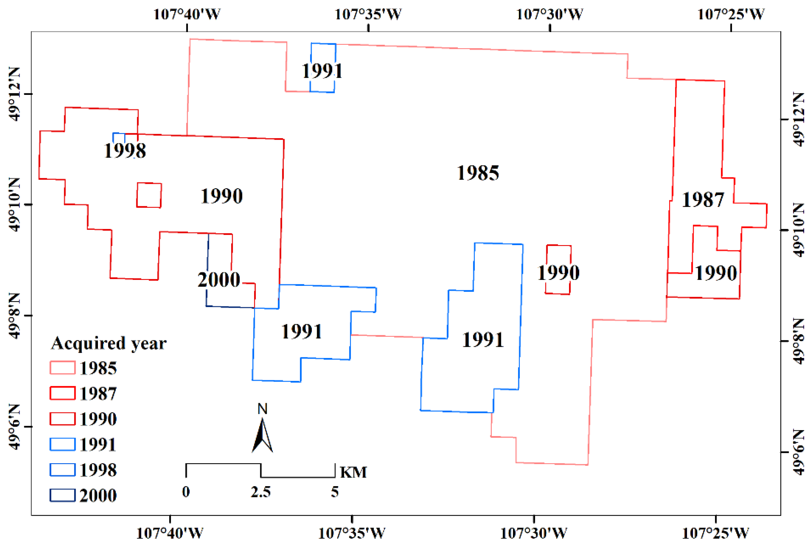
3.1.1. Landsat Images for Temporal Analysis

A total of 126 cloud-free Landsat images (Table 1), including 2 Thematic Mapper (TM) images from Landsat 4, 87 TM images from Landsat 5, 12 Enhanced Thematic Mapper Plus (ETM+) images from Landsat 7, and 25 Operational Land Imager (OLI) images from Landsat 8, were collected from 1986 to 2020 (i.e., only images acquired from April to October were used for temporal analysis to avoid ice and snow cover). All Landsat images were preprocessed (i.e., with both geometric and atmospheric correction; Level 2 data from Landsat Collection 2) when downloaded from the United States Geological Survey (USGS) website (https://earthexplorer.usgs.gov/, accessed on 14 January 2020).
According to the Level 2 data information from Landsat Collection 2 (https://www.usgs.gov/core-science-systems/nli/landsat/landsat-collection-2-level-2-science-products, accessed on 20 April 2021), the algorithm for generating surface reflectance data from Collection 2, Level 1 products of Landsat 4-5 TM and Landsat 7 ETM+ was the Landsat Ecosystem Distribution Adaptive Processing System (LEDAPS) algorithm (Version 3.4.0), and that of Landsat 8 OLI was the Land Surface Reflectance Code (LaSRC) algorithm (Version 1.5.0). The spatial resolution of all Landsat images was 30 × 30 m, which were projected as UTM Zone 13N, WGS1984. The pixel values of multispectral bands from the Level 2 products were converted to surface reflectance with a scaling factor of “0.0000275 × pixel value − 0.2” (e.g., if the pixel value is 32,000, the reflectance is 0.68). Pixel values of thermal bands from Landsat Collection 2, Level 2, were converted to surface temperature with a scaling factor of “0.00341802 × pixel value + 149.0 − 273.15” (e.g., if the pixel value is 45,000, the surface temperature is 29.6609 °C; the thermal band of Landsat 8 used in this study is band 10).

3.1.2. Sentinel-2 Images and DEM Image for Classification

Eleven Sentinel-2 images acquired in 2018 (i.e., all the available cloud-free images in the growing season from April to October) were downloaded from the USGS website (https://earthexplorer.usgs.gov/, accessed on 16 January 2020). The downloaded images (acquisition dates 2018-04-28, 2018-05-03, 2018-05-13, 2018-06-12, 2018-06-27, 2018-07-07, 2018-07-17, 2018-08-11, 2018-08-16, 2018-09-05, and 2018-10-20) were Level 1 products of Sentinel-2 images and geometrically corrected. All Sentinel-2 images were then radiometrically and atmospherically corrected using the Sen2Cor toolbox from SNAP software provided by the European Space Agency (ESA), and resampled to a spatial resolution of 30 m.
Digital Elevation Model (DEM) data were from the Global Digital Elevation Model V002 (GDEM2) from Advanced Spaceborne Thermal Emission and Reflection Radiometer (ASTER), downloaded from the NASA website (https://reverb.echo.nasa.gov/reverb/, accessed on 20 April 2021). DEM data for GNP was projected as Universal Transverse Mercator (UTM) Zone 13N, WGS1984 (World Geodetic System 1984) with a spatial resolution of 30 m.

3.2. Methodology

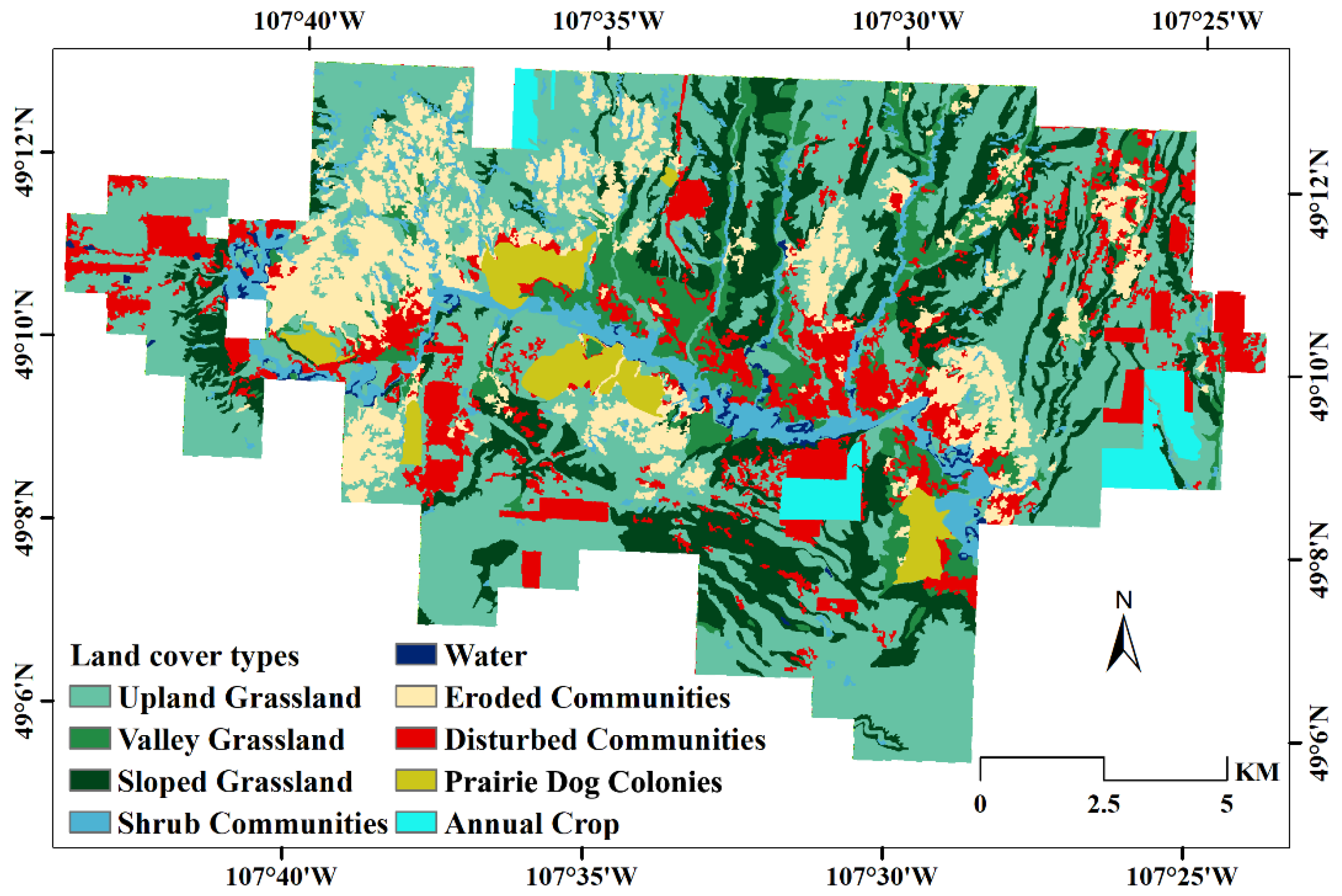
3.2.1. Classification of Vegetation Communities

We conducted Principal Component Analysis (PCA) to the band composition of the DEM image and all eleven Sentinel-2 images (i.e., Normalized Difference Vegetation Index (NDVI) calculated for each Sentinel-2 image before PCA). The first band from PCA results was excluded before unsupervised classification because this band largely consists of DEM information instead of vegetation. An ISO unsupervised classification based on ArcGIS 10.5 software was applied to the band composition of PCA results excluding the first component. Post-classification techniques, including reclassification, majority filter, boundary clean, region group and nibble were also applied to the classification results to improve the results for vegetation communities. The information from prairie dog towns, annual crops, and some disturbed communities were incorporated into classification results based on 1983 and 1995 field surveys [53]. The overall accuracy for the final classification map of vegetation communities (Figure 2) was 89.7%, based on 100 randomly distributed sample points using visual interpretation.

3.2.2. Links between Surface Reflectance of Landsat Images and Grassland Biophysical Parameters

Our previous research on prairie responses to grazing cessation in GNP [50] indicated that the difference of biophysical parameters of conserved and grazed sites had a linear relationship with the difference of surface reflectance (or land surface temperature) in Landsat bands. This research showed that the difference in near-infrared (NIR) reflectance, first shortwave infrared (SWIR1) reflectance and second shortwave infrared (SWIR2) reflectance, and land surface temperature (LST) from the thermal band, are all significantly correlated with the differences of fresh biomass, soil organic matter, green cover and litter cover (Table 2), respectively [50]. Therefore, we used these relationships as indicators of the prairie response to grazing management, considering the potentially overwhelming influence of climate change.

3.2.3. Formation of Time Series Dataset by “Zoo Objects” and Missing Value Interpolation

Time series datasets were prepared using “zoo objects” in the R software package (https://www.r-project.org/, accessed on 16 March 2020) for each pixel of NIR, SWIR1, and SIWR2 reflectance and LST. First, a raster time series object was generated from a raster stack object in the 126 Landsat images and the corresponding acquisition date for each image in R software. Then, a time series dataset was formed for each pixel using a “for loop” in the zoo package. To do this, the temporal dataset for each pixel was aggregated into monthly data using the “aggregate” function (i.e., if more than one image was acquired in the same month, their data were aggregated by their mean value). This aggregated temporal dataset had missing values in the months for which cloud-free Landsat images were unavailable. To form a regular “zoo object”, each pixel was assigned a specific frequency of 7 (the number of acquisition months from April to October). The missing values for each pixel were then interpolated using a seasonal Kalman filter (the na.StructTS() function in the zoo package). The seasonal Kalman filter has been shown to be a functional method to filter missing values in a dataset with repeated seasonal variability [54]. As a final step, the regular zoo object for each pixel of NIR, SWIR1, SWIR2, and LST was generated without any missing values. NDVI is the most popular vegetation index for representing green vegetation information [55,56], and Normalized Difference Water Index (NDWI) is a good indicator for plant water content [57,58,59]. Therefore, in addition to these four bands, the regular zoo objects for NDVI [60] Equation (1) and NDWI [61] Equation (2) were also generated.
N D V I = ( N I R R ) / ( N I R + R )
where NDVI refers to the normalized difference vegetation index, NIR refers to the near-infrared band (i.e., band 4 for TM and ETM+ images and band 5 for OLI images); R refers to the red band (i.e., band 3 for TM and ETM+ images and band 4 for OLI images).
N D W I = ( N I R S W I R 1 ) / ( N I R + S W I R 1 )
where NDWI refers to normalized difference water index, SWIR1 refers to the first shortwave infrared band (i.e., band 5 for TM and ETM+ images and band 6 for OLI images).

3.2.4. Pixel Based Time Series Analysis

Based on the filtered regular zoo object for each pixel, a time series object was formed for each pixel (i.e., start in 1986 with a frequency of 7) using the “ts” function in the raster time series (rts) package from the R software. Time series analysis was then applied to decompose the temporal object of each pixel into trend component, seasonal component, and random noise component using the “stl” function in the “rts” package. With time series analysis, seasonal variation is minimized for maintaining temporal consistency of long-term studies [47]. The median value into the trend component of each pixel was extracted to calculate a new raster for each year. The NIR, SWIR1, SWIR2, LST, NDVI, and NDWI, with limited seasonal effects for these rasters, were used for further temporal analysis.

3.2.5. Segmented Linear Regression

Zonal statistics in ArcGIS 10.5 were applied to calculate the mean values of newly generated rasters for each year from 1986 to 2020. We did this using polygons formed from the intersection of different vegetation communities (Figure 2) and the land acquisition year (Figure 1). Then, temporal trends (for NIR, SWIR1, SWIR2, LST, NDVI, and NDWI independently) were calculated based on the mean value of zonal statistic results (see the selection of three vegetation types in the surrounding pastures in Supplementary, Figure S1). The temporal trends of the difference in each multispectral band and index for a certain vegetation community were calculated by using the temporal trend of the GNP sites (acquired in 1985) minus that of the surrounding pastures. Then, the temporal trends of the difference in NIR, SWIR1, SWIR2, LST, NDVI, and NDWI between 1985 and 2020 was smoothed by the loess function in R software. Finally, the segmented linear regression in the “segmented” package in R software was applied to each smoothed temporal trend to evaluate the significant turning points. The segmented linear relationship (i.e., broken-line relationship) has a variety of applications in ecological research [51]. In this study, the segmented linear relationship was used to analyze thresholds for the optimum duration of prairie restoration practices including grazing cessation and reintroduction. After the turning points were measured for each smoothed trend, the slope was calculated for each line segment to analyze the intensity of the influences of grazing cessation and the reintroduction of the three native vegetation communities.

4. Results

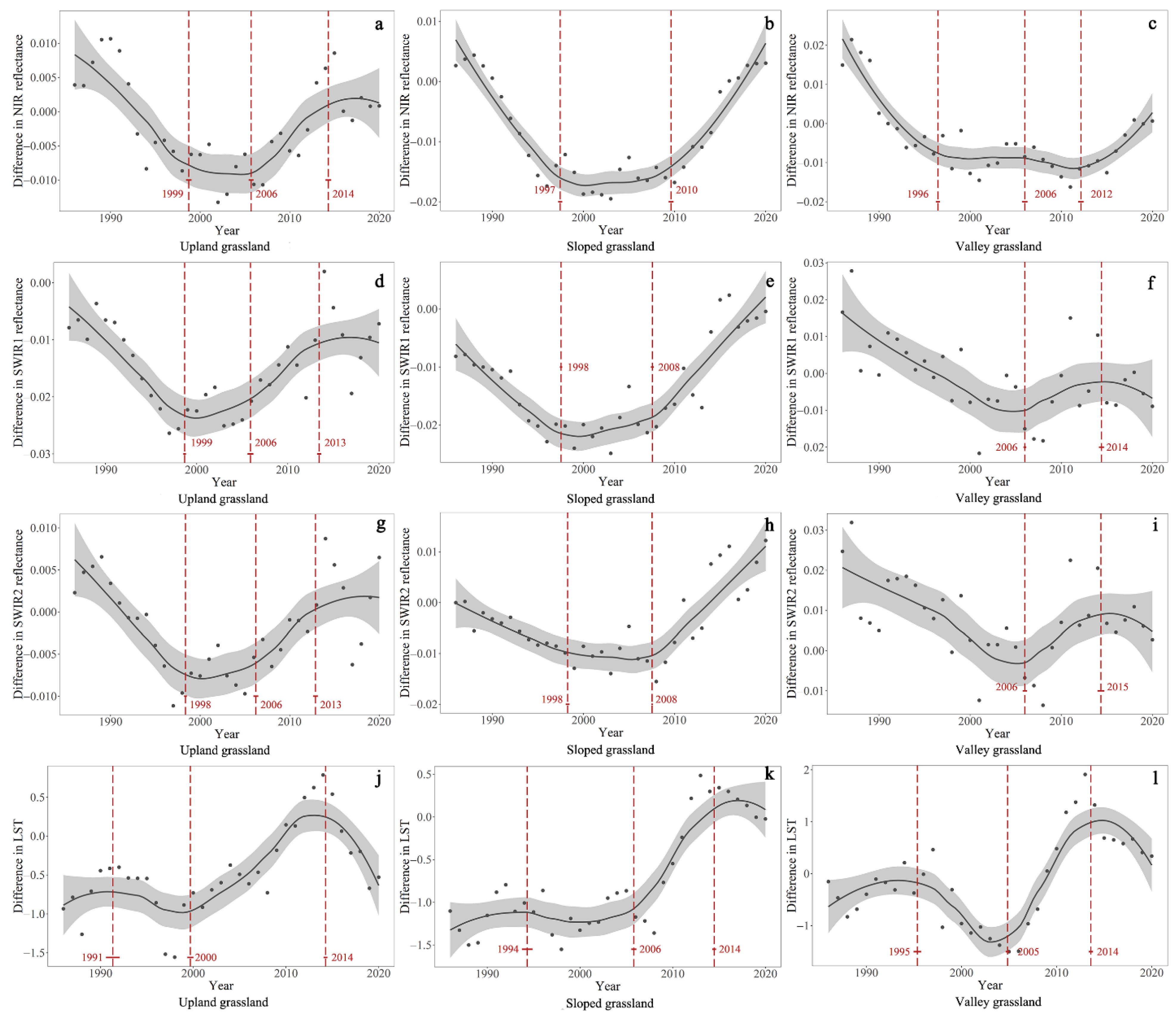
4.1. Temporal Trends of the Difference in NIR, SWIR1, SWIR2, and LST between GNP and Surrounding Pastures

NIR reflectance of upland, sloped, and valley grasslands in GNP was higher than that of surrounding pastures in 1985 (the year GNP was first acquired as a national park), based on the temporal trend of the difference in NIR reflectance between GNP sites and the surrounding pastures (Figure 3a–c). The difference in NIR reflectance gradually decreased until it reached a relatively stable stage when GNP was under grazing cessation from 1985 to 2006 (Figure 3a–c). However, the effective time periods for the impact of grazing cessation on three vegetation communities were different. The time periods when grazing cessation caused a significant change in the difference in NIR for upland, sloped, and valley grasslands were 1985–1999, 1985–1997, and 1985–1996, respectively (Table 3; Figure 3a–c). During the effective time periods, valley grassland had the strongest response to grazing cessation (the absolute slope is 0.0029 of the first linear segment; Table 3), while upland grassland (the absolute slope is 0.0014 of the first linear segment; Table 3) and sloped grassland (the absolute slope is 0.0021 of the first linear segment; Table 3) had a milder response to grazing cessation based on the temporal dynamics of the difference in NIR reflectance. After these time periods, grazing cessation had no statistically significant influences on the three vegetation communities anymore (Figure 3a–c). After bison were reintroduced in 2006, the temporal trend of the difference in NIR reflectance for upland grassland changed in reverse of the initial changes when it first began to be conserved in 1985, while it became stable after 2014, 8 years after grazing reintroduction was implemented (Figure 3a). However, the difference in NIR reflectance remained stable for the first four and six years for sloped and valley grasslands, respectively, and then increased afterwards when they were under grazing reintroduction management (Figure 3b,c). Grazing reintroduction had a stronger impact on sloped and valley grasslands (absolute slope of second linear segment is 0.002 for sloped grassland and 0.0019 for valley grassland; Table 3) than upland grassland (absolute slope of first linear segment is 0.0013; Table 3).
Except in the valley grassland, the difference in SWIR1 reflectance for upland and sloped grasslands in GNP in 1985 was lower than the surrounding pastures (Figure 3d–f). Grazing cessation caused a significant decrease in the difference in SWIR1 reflectance between GNP and the surrounding pastures in the first 14 years for upland grassland (1985–1999; Figure 3d) and in the first 13 years for sloped grassland (1985–1998; Figure 3e). According to the temporal changes on the difference in SWIR1 reflectance, the intensity of the impact of grazing cessation was slightly stronger in upland grassland than in sloped grassland (i.e., the absolute slope of the first linear segment for upland and sloped grassland were 0.0016 and 0.0014, respectively; Table 3). After these time periods, grazing cessation caused the difference in SWIR1 reflectance increasing with a much milder intensity (Figure 3d,e; the absolute slope of the second linear segment for upland and sloped grassland were 0.0004 and 0.0003, respectively). The impact of grazing cessation on the difference in SWIR1 reflectance did not show a time lag effect for valley grassland; instead, it caused a continuous decrease in the temporal trend of SWIR1 difference from 1985 to 2006 until grazing reintroduction broke the temporal trend (Figure 3f). After bison were reintroduced in GNP, the difference in SWIR1 increased for upland grassland during 2006–2013, for sloped grassland during 2006–2020, and for valley grassland during 2006–2014 (Figure 3d–f). The impact of grazing reintroduction was stronger for upland and sloped grasslands than it was for valley grassland (i.e., the absolute slope of the first linear segment was 0.0014, 0.0017, and 0.0009 for upland, sloped and, valley grasslands, respectively; Table 3). However, grazing reintroduction was no longer effective for upland grassland since 2013, and was much less effective for valley grassland after 2014 (Figure 3d–f).
In 1985, the difference in SWIR2 reflectance for upland and valley grasslands in GNP was higher than the surrounding pastures, and sloped grassland was almost the same for both GNP and surrounding pastures (Figure 3g–i). Grazing cessation caused a significant decrease in the difference in SWIR2 reflectance between GNP and the surrounding pastures in the first 13 years for both upland and sloped grasslands (1985–1998; Figure 3g,h). However, the intensity of the impact of grazing cessation on the difference in SWIR2 reflectance was greater for upland grassland than for sloped grassland (i.e., the absolute slope of the first linear segment was 0.0012 and 0.0008 for upland and sloped grasslands, respectively; Table 3). The temporal trend of the difference in SWIR2 during grazing cessation implementation period did not show a statistically significant turning point for valley grassland, instead, grazing cessation caused a continuous decrease in the difference of SWIR2 reflectance from 1985 to 2006 (Figure 3i). Since 2006, when the grazing reintroduction was implemented, the difference in SWIR2 increased for upland grassland during 2006–2013 and valley grassland during 2006–2015 (Figure 3g,i), while it continued to increase for sloped grassland from 2008 to 2020 (Figure 3h). Grazing reintroduction had the strongest effects on the difference in SWIR2 reflectance for sloped grassland (the absolute slope of the linear regression was 0.0017; Table 3) than upland and valley grasslands (the absolute slope of the first linear segment for upland and valley grasslands was 0.0014 and 0.0009, respectively; Table 3).
Grazing cessation had no significant impact on the difference in LST for upland grassland in the first 6 years, for sloped grassland in the first 9 years, and for valley grassland in the first 10 years (Figure 3j–l; Table 3). However, after these periods, the difference in LST between GNP and surrounding pastures slightly dropped while GNP was continuously under grazing cessation (Figure 3j–l). Valley grassland had the greatest decline in the difference in LST between 1995 and 2005 (i.e., the absolute slope of the second linear segment is 0.11; Table 3), followed by upland and sloped grasslands (i.e., the absolute slopes of the second linear segment are 0.04 and 0.01 for upland and sloped grasslands, respectively; Table 3). Grazing reintroduction had much stronger influences on the temporal trend of the difference in LST (Figure 3j–l). Since 2006, grazing reintroduction caused the difference in LST to increase until 2014, with a linear slope of 0.1, 0.15, and 0.25 for upland, sloped, and valley grasslands, respectively (Table 3).

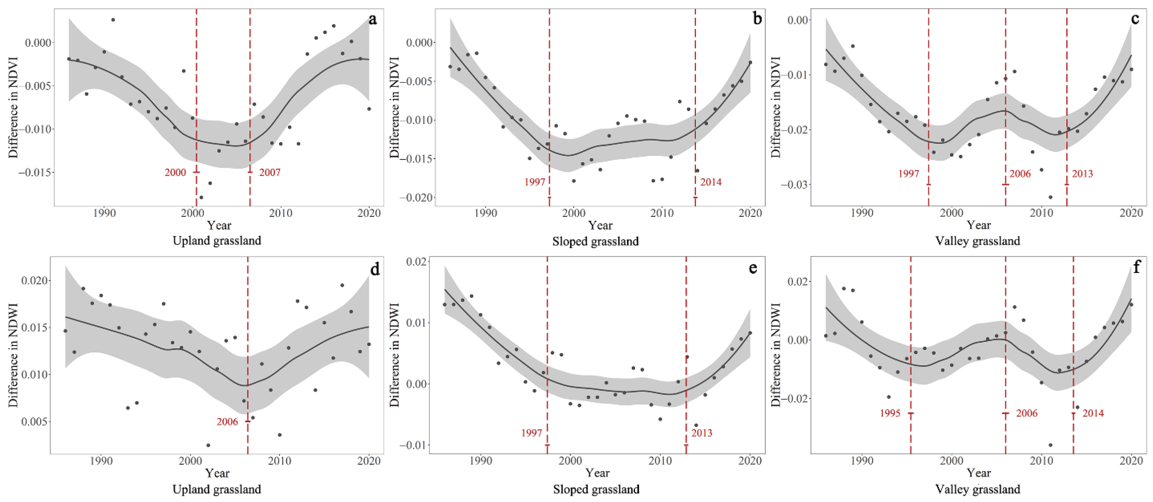
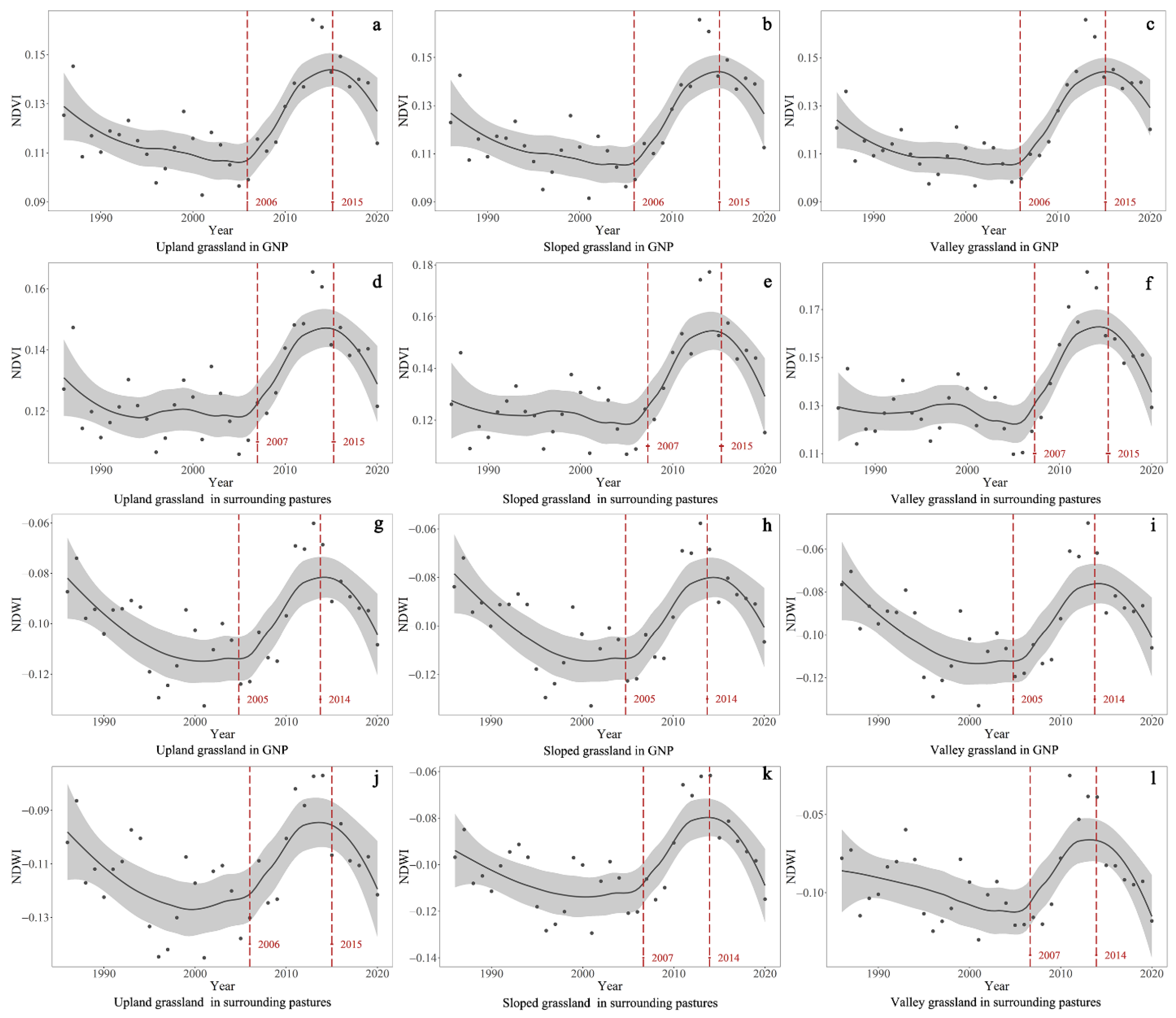
4.2. Temporal Trends of the Differences in NDVI and NDWI between GNP and Surrounding Pastures

The difference in NDVI gradually decreased in upland during 1985–2000, in sloped grassland during 1985–1997, and in valley grassland during 1985–1997 (Figure 4a–c). The decreasing pace for valley grassland is larger than that for upland and sloped grasslands (i.e., the absolute slope of the first linear segment is 0.0007, 0.0012, and 0.0015 for upland, sloped, and valley grasslands, respectively; Table 4). After these periods, the difference in NDVI of upland and sloped grasslands became stable, while grazing cessation influenced the difference in NDVI of valley grassland in an opposite direction of the initial changes after 1997 (Figure 4a–c; Table 4).
After bison were reintroduced in GNP in 2006, the difference in the NDVI increased in upland grassland (Figure 4a), while it remained stable in sloped grassland until 2014 and decreased in valley grassland until 2013 (Figure 4b,c). After these time periods, grazing reintroduction increased the difference of NDVI in sloped and valley grasslands (Figure 4b,c; Table 4).
The temporal trends of the difference in NDWI show similar trends with NDVI, though different turning points and intensity between sloped and valley grasslands when both communities were under grazing cessation and reintroduction managements (Figure 4e,f; Table 4). In upland grassland, the difference in NDWI gradually decreased during the whole period of grazing cessation and increased grazing reintroduction from 2006 to 2020 (Figure 4d).

5. Discussion

5.1. Monitoring Prairie Management Effects Using a Landsat Imagery Raster Time Series Analysis

Long-term temporal analysis has been shown to be essential to monitor prairie responses to management change. However, temporal inconsistency in image series challenges long-term analysis when using remotely sensed imagery in prairie research. Previous studies have used images acquired in the maximum growing season to analyze temporal dynamics of ecosystems [42]. However, the low temporal resolution of Landsat images may miss the reflectance of the peak growth due to the short northern prairie growing season [43]. The maximum growing season corresponds to rainfall peaks, resulting in large intervals of cloud cover and missing data during key growing periods. The short lags between rainfall and grassland community growth confounds the consistent use of remote sensing in prairie ecosystems.
Seasonal variation also affects the temporal monitoring of prairie ecosystems because of vegetation phenology. We applied a seasonal Kalman filter to fill missing values caused by cloud effects based on the seasonal cycles in long-term Landsat images. These vary across vegetation communities with different penology [54]. The pixel-based seasonal Kalman filter was applied to generate the regular time series raster object and minimize the effects of seasonal variation among vegetation communities. The filter generated better time series data than spline interpolation in particular during a year with many missing images. Temporal trends were separated by time series analysis to eliminate the seasonal effects [47], which greatly enhanced the temporal consistency of the reflectance of Landsat images.

5.2. The Relationship between the Difference in Biophysical Parameters and Multispectral Reflectance

Green vegetation cover [62,63,64] and biomass [65,66,67] are two of the most common biophysical indicators used to evaluate management responses in prairie ecosystems. These have been estimated using statistical models based on field-measured data and spectral indices based on red, NIR, or SWIR1 bands [68]. In GNP, a large amount of non-photosynthetic materials challenges estimates of fresh biomass and green cover from Landsat images [69]. We were able to take advantage of our previous research relating to the difference in NIR and SWIR2 reflectance and the difference in fresh biomass and green cover between GNP sites and the surrounding pastures, respectively [50]. Soil organic matter and litter cover are two indicators that are not easily measured using Landsat reflectance [58], yet play a strong role in prairie management. Previous research shows that SWIR1 reflectance is well correlated to soil organic matter [50,70,71]. Litter accumulation decreases LST [50], which is consistent with the ecological function of litter that enhances soil moisture and mitigates soil surface temperature [51]. Therefore, we take advantage of the results from our previous research [50] to use the difference in NIR, SWIR1, SWIR2, and LST to predict the difference in fresh biomass, soil organic matter, green cover, and litter cover between GNP and the surrounding pastures, respectively (Table 2). More importantly, it highly reduced the effects of climate change by using the temporal trends of the difference in NIR, SWIR1, SWIR2, and LST for the vegetation communities in GNP and the surrounding grazing pastures, because the same vegetation type in GNP and the surrounding pastures was under the same intensity of climate change for a given time, albeit under different management policies.
Our previous research [50] used the five paired ecological comparison sites (i.e., all the sites are upland grasslands) in GNP and the surrounding pastures to form the linear relationship between the difference in NIR, SWIR1, SWIR2, and LST and the difference in fresh biomass, soil organic matter, green cover, and litter cover, respectively (Table 2). Each paired site has similar vegetation composition and soil properties, therefore, the difference in NIR, SWIR1, SWIR2, and LST were mainly caused by difference management policies between GNP and the surrounding pastures. However, there are still some biases and uncertainties when using the difference in NIR, SWIR1, SWIR2, and LST between GNP and the surrounding pastures. First, the linear models of the difference in Landsat reflectance and the difference in biophysical parameters did not exactly fit the assumption of homoscedasticity, which would reduce the statistic power. Second, it would bring uncertainties by directly applying those linear models on Landsat TM, ETM+ and OLI images, because the initial linear models were built based on Landsat TM images and field data (Table 2). Third, the limited samples of field data also make the linear models less reliable (i.e., 8 paired samples for fresh biomass and soil organic matter collected in 2004 and 2005, and 13 paired samples for green cover and litter cover collection in 2003, 2004, and 2005). Fourth, when this study was extended into the whole study area, the heterogeneity of the mixed prairie makes it impossible to find the pixels in the surrounding pastures, which have similar vegetation composition and soil properties to pair each of the pixels of GNP sites, including upland, sloped, and valley grasslands. The difference data used in this study was calculated by the mean value of upland, sloped, and valley grasslands in GNP minus the mean value of typical upland, sloped, and valley grassland in the surrounding pastures, respectively. However, the inconsistency of species composition, soil properties and canopy information would bring biases to the difference in the temporal trends between GNP and surrounding pastures. Finally, the accuracy of vegetation classification (Figure 2) also brought bias to the results because the calculation of the mean value of difference vegetation communities relies on the classification results. The accuracy of our classification map (89.7%) might have some biases because it was conducted by visual interpretation of 100 random points instead of field validation data.

5.3. The Impact of Grazing Cessation on Three Native Vegetation Communities

According to the positive linear relationship between the difference in fresh biomass and NIR reflectance (Table 2), the difference of NIR reflectance between GNP sites and the surrounding pastures indicates a higher fresh biomass in the park than that of the surrounding pastures in 1985, when GNP was first acquired for all three vegetation types (Figure 3a–c). The impact of grazing cessation on the temporal dynamics of the difference in NIR reflectance indicates that grazing cessation, compared to moderate grazing management in the surrounding pastures, decreased fresh biomass in upland, sloped, and valley grassland within a certain time period of 11–14 years, varying from different vegetation communities (Figure 3a–c; Table 3). The intensity of grazing cessation on fresh biomass varies from three vegetation communities as well. Under the implementation of grazing cessation, the difference in fresh biomass between GNP and surrounding pastures decreased 30.24 g for upland grassland during 1985–1999, 38.88 g for sloped grassland during 1985–1997, and 49.22 g for valley grassland during 1985–1996 (i.e., calculated based on slope of the linear segment and positive linear relationship between the difference in fresh biomass and the difference in NIR reflectance; Table 2 and Table 3). The stability of the temporal trend of the difference in NIR reflectance after those time periods suggests no effectiveness of grazing cessation on fresh biomass (Figure 3a–c; Table 3).
The decrease in the difference of SWIR1 reflectance reveals the increase in the difference of soil organic matter between GNP and the surrounding pastures, caused as a result of the negative linear relationship between the difference in soil organic matter and the difference in SWIR1 reflectance (Table 2). Compared to the moderate grazing management in the surrounding pastures, grazing cessation increased soil organic matter in upland grassland for the first 14 years and in sloped grassland for the first 13 years, while it continuously increased soil organic matter in valley grassland for all 21 years under grazing cessation. The intensity of the impact of grazing cessation on GNP varies from different vegetation types as well. Grazing cessation caused an increase in soil organic matter by 0.51% for upland grassland, 0.55% for sloped grassland, and 5.73% for valley grassland (Table 2 and Table 3).
Our previous research shows that the difference in green cover between GNP sites has a negative linear relationship with the difference in SWIR2 reflectance (Table 2). Thus, the decrease in the difference of SWIR2 reflectance indicates an increase in the difference of green cover between GNP and the surrounding pastures for upland and sloped grasslands during 1985–1998, as well as for valley grassland during all 21 years under grazing cessation (Figure 3g–i), compared to the moderate grazing management in the surrounding pastures. However, the intensity of the influences of grazing cessation on green cover varies for three vegetation communities. Grazing cessation caused an increase in green cover by 5.43% for upland grassland, 3.62% for sloped grassland, and 9.50% for valley grassland (Table 2 and Table 3).
The differences in NIR, SWIR1, and SWIR2 between GNP and the surrounding pastures have shown similar temporal trends as those seen in previous research [50]. However, the difference in LST does not show similar temporal trends with our previous research, which indicates that other factors besides litter cover, including species composition, vegetation canopy, water content, and soil properties, might override the effects of litter cover difference on LST.
When using fresh biomass, soil organic matter, and green cover as indicators, grazing cessation had the strongest impact on valley grassland and the mildest impact on sloped grassland, mostly within a time period of 11 to 14 years instead of the whole management period. This may be because the vegetation in valley grasslands have a higher above-ground biomass and height, with more accumulation of soil organic matter. It is also possible that greater moisture in the valley grassland would increase the decomposition of dead material, resulting in more green cover due to less competition for growing space with standing dead materials [51]. The increase in the difference of soil organic matter and green cover suggests that grazing cessation is more effective than long-term moderate grazing management (i.e., a management policy for the surrounding pastures). The decrease in the difference of fresh biomass when GNP was under grazing cessation management is due to a large amount of accumulation of non-photosynthetic materials.
The decrease in the difference of NDVI and NDWI when GNP was under grazing cessation is also due to dead material accumulation, as it is generally a restoration objective of grazing cessation in prairies [8]. Based on the temporal trends of the difference in NDVI and the difference in NDWI, grazing cessation influenced upland grassland with the longest period but the mildest intensity, while it impacted valley grassland with the shortest time period but the largest intensity among all three vegetation communities (Figure 4 and Table 4). However, the difference between GNP and the surrounding pastures was not visibly obvious in NDVI or NDWI images, while the difference was clear in NIR, SWIR1, and SWIR2 bands, especially the NIR band (see Supplementary, Figure S1 for the images acquired in 2006).

5.4. The Impact of Grazing Reintroduction on Three Native Vegetation Communities

Based on the temporal trend in the difference of NIR reflectance (Figure 3a–c) and the relationship between fresh biomass and NIR reflectance (Table 2), grazing reintroduction increased fresh biomass by 16.05 g during 2006–2014 for upland grassland and then became stable (Figure 3a), while it was not effective for fresh biomass in sloped grassland for the first 4 years and valley grassland for the first 6 years (Figure 3b,c). After the first stable stage, grazing reintroduction increased fresh biomass by 30.86 g in sloped grassland from 2010–2020 and by 23.45 g in valley grassland from 2012–2020 (Table 2 and Table 3). The impact of grazing reintroduction was slightly better at enhancing fresh biomass in sloped and valley grasslands than in upland grassland, compared to moderate grazing management.
Grazing reintroduction decreased soil organic matter by 1.78% in upland grassland from 2006 to 2013 and by 1.31% in valley grassland between 2006 and 2014, while it continuously decreased soil organic matter by 3.71% in sloped grassland until 2020 (Table 2 and Table 3). Compared to grazing cessation, soil organic matter restored in at the slowest pace in sloped grassland (absolute slope of the first linear segment is 0.0014; Table 3). Among three vegetation types, however, it degraded at the highest speed while it was under grazing reintroduction management (absolute slope of the first segment is 0.0017; Table 3). The impact of grazing reintroduction on soil organic matter for valley grassland was the mildest among the three vegetation types.
Since 2006, the year grazing reintroduction was implemented in GNP, green cover decreased by 2.44% in upland until 2013, by 5.01% in valley grassland until 2015, and by 7.52% in sloped grassland until 2020 (i.e., no clear time lag effects showed for sloped grassland). For sloped grassland, green cover recovered in the slowest pace under grazing cessation, but it decreased in the highest speed under grazing reintroduction among the three vegetation types (Table 3).
According to the changes of the fresh biomass, soil organic matter, and green cover, grazing reintroduction had a shorter effective time period and milder intensity than grazing cessation for upland and valley grasslands (Figure 3; Table 2 and Table 3). Among all three types, grazing reintroduction had the greatest intensity of impact on sloped grassland and the smallest intensity of influences on valley grassland. For sloped grassland, grazing reintroduction had stronger effects than grazing cessation in a reversed direction.
Based on the temporal trends of the difference in NDVI and NDWI between GNP sites and surrounding pastures, grazing reintroduction influenced upland grassland for the longest period but with the mildest intensity, while it was effective on sloped and valley grassland, with a time lag of 7 to 8 years (Figure 4 and Table 4). After 7 to 8 years under grazing reintroduction management, the differences between NDVI and NDWI in sloped and valley grasslands changed in an opposite direction, just as GNP did under grazing cessation (Figure 4). This phenomenon was shown in the temporal trend of the difference in NIR reflectance, as well in sloped and valley grasslands (Figure 3b,c). This may be due to the selective grazing by bison in the first few years when they were first introduced into GNP [50].
The dynamics of the most temporal trends of the differences in Landsat bands or indices indicates that grazing reintroduction returned upland, sloped, and valley grasslands to their initial stage in 1985 in less time than the time of the maximum changes caused by grazing cessation (Figure 3 and Figure 4).

5.5. The Influences of Climate Change on Three Native Vegetation Communities

It is generally a challenge to separate the influences of climate change and prairie management with remote sensing applications, using biophysical parameters as indicators to evaluate the response to climate change or prairie management. With long-term Landsat images, the temporal trends of different vegetation indices were often used to analyze the impact of prairie management or climate change. However, vegetation communities have similar temporal trends of NDVI and NDWI (Figure 5), suggesting that climate effects have a high potential to override the impact of prairie management (i.e., the grazing cessation and reintroduction in this study).
When analyzing the temporal trends of NIR, SWIR1, SWIR2, and LST for three native vegetation communities in GNP, the increase in NIR, SWIR1, and SWIR2 reflectance and LST reveals an increase in fresh biomass, and a decrease in soil organic matter, green cover, and litter cover, respectively, to some extent. However, other factors, including water content and global warming, would influence the variation of the temporal trends of Landsat reflectance and LST. The vegetation communities in GNP have similar temporal trends of NIR, SWIR1, SWIR2, and LST, as those in the surrounding pastures (Supplementary, Figures S2–S5); however, the different change rates still reveal the impact of grazing cessation and reintroduction. Therefore, the differences in Landsat reflectance and vegetation indices are good options with which to analyze the influences of prairie management only. LST temporal trends were similar for the three native vegetation communities in GNP and the surrounding pastures (Supplementary, Figure S5), which suggests that their dynamics may be dominated by climate change. The air temperature recorded at the closest meteorological station did not show an annual mean temperature increase from 1985 to 2020, however, the monthly mean temperature for prairie growing season (i.e., June to August) increased by 0.46 ℃ per year from 1985 to 1999 and stabilized from 2000 to 2020. The continuous increase in LST was consistent with air temperature.

6. Conclusions

Grazing cessation has been suggested as a superior prairie management policy to long-term moderate grazing for enhancing soil organic matter and increasing green cover. Among all three native vegetation communities, grazing cessation had a stronger impact on valley grasslands and the mildest effects on sloped grasslands. The significantly effective time period of grazing cessation to occur differed among biophysical indicators and vegetation communities in GNP, which were 11 to 14 years. Grazing cessation increased soil organic matter for 14 and 13 years for upland and sloped grasslands, respectively; increased green cover for 13 years for both upland and sloped grasslands; decreased fresh biomass for 14, 12, and 11 years for upland, sloped, and valley grasslands, respectively.
Grazing reintroduction affected the prairie ecosystem with a shorter effective time period than grazing cessation for both upland and valley grasslands. The intensity of grazing reintroduction was strongest in sloped grasslands and mildest in valley grasslands. Grazing reintroduction had weaker influences on upland and valley grasslands, but stronger effects on sloped grassland than on grazing cessation. The effective time period of grazing reintroduction was 7 to 9 years for upland and valley grasslands, while there was no clear time lag effect in sloped grassland.
Generally, the increase in NDVI and NDWI is an indicator of restoration outcome for grazing cessation. However, the opposite temporal trends of NDVI and NDWI were observed in this study when GNP was under grazing cessation. This is because the continuously accumulated non-photosynthetic materials highly reduced the reflectance in NIR, an important band for calculating NDVI and NDWI.
The results of our study provide fundamental information for prairie mangers on the effects of grazing cessation and reintroduction compared to long-term moderate grazing management. More importantly, the results of this study suggest the time periods for management to take effect among grassland communities.

Supplementary Materials

The following are available online at https://www.mdpi.com/article/10.3390/rs13173397/s1, Figure S1: Selection of three vegetation types in the surrounding pastures; Figure S2: NIR reflectance of upland, sloped, and valley grasslands from both GNP and the surrounding pastures; Figure S3: SWIR1 reflectance of upland, sloped, and valley grasslands from both GNP and the surrounding pastures; Figure S4: SWIR2 reflectance of upland, sloped, and valley grasslands from both GNP and the surrounding pastures; Figure S5: LST of upland, sloped, and valley grasslands from both GNP and the surrounding pastures.

Author Contributions

Conceptualization, D.X. and X.G.; methodology, D.X. and J.K.H.; validation, D.X., W.X. and X.G.; formal analysis, D.X.; investigation, D.X. and X.G.; writing—original draft preparation, D.X.; writing—review and editing, J.K.H., W.X. and X.G.; supervision, X.G.; funding acquisition, D.X., W.X. and X.G. All authors have read and agreed to the published version of the manuscript.

Funding

This research was funded by the Natural Science and Engineering Research Council of Canada (GRPIN-2016-03960), the Natural Science Foundation of Jiangsu Province (BK20180769), the Science and Technology Project Funds of Qinghai Province (2019-HZ-820), the Major Basic Research Project of the Natural Science Foundation of the Jiangsu Higher Education Institutions (18KJB180009), and the Science and Technology Program Project Funds of Sichuan Province (2019YFS0465).

Institutional Review Board Statement

Not applicable.

Informed Consent Statement

Not applicable.

Acknowledgments

The authors would like to acknowledge Grasslands National Park for the logistical support. We also acknowledge John Wilmshurst for editing and polishing the English for this manuscript.

Conflicts of Interest

The authors declare no conflict of interest.

References

  1. Alemu, A.W.; Kröbel, R.; McConkey, B.G.; Iwaasa, A.D. Effect of Increasing Species Diversity and Grazing Management on Pasture Productivity, Animal Performance, and Soil Carbon Sequestration of Re-Established Pasture in Canadian Prairie. Animals 2019, 9, 127. [Google Scholar] [CrossRef] [Green Version]
  2. Milton, S.J.; Dean, W.J.; Ellis, R.P. Rangeland health assessment: A practical guide for ranchers in arid Karoo shrublands. J. Arid. Environ. 1998, 39, 253–265. [Google Scholar] [CrossRef]
  3. Follett, R.; Stewart, C.; Bradford, J.; Pruessner, E.; Sims, P.L.; Vigil, M. Long-term pasture management impacts on eolian sand soils in the southern mixed-grass prairie. Quat. Int. 2020, 565, 84–93. [Google Scholar] [CrossRef]
  4. Bajgain, R.; Xiao, X.; Basara, J.; Doughty, R.; Wu, X.; Wagle, P.; Zhou, Y.; Gowda, P.; Steiner, J. Differential responses of native and managed prairie pastures to environmental variability and management practices. Agric. For. Meteorol. 2020, 294, 108137. [Google Scholar] [CrossRef]
  5. Ruggiero, N.; Kral, G.L. Prescribed cattle grazing as a tool for native prairie management: Lessons from the Tualatin River basin, Oregon. J. Soil Water Conserv. 2018, 73, 74A–78A. [Google Scholar] [CrossRef] [Green Version]
  6. Dunwiddie, P.W.; Bakker, J.D. The Future of Restoration and Management of Prairie-Oak Ecosystems in the Pacific Northwest. Northwest Sci. 2011, 85, 83–92. [Google Scholar] [CrossRef]
  7. Dennehy, C.; Alverson, E.R.; Anderson, H.E.; Clements, D.R.; Gilbert, R.; Kaye, T.N. Management Strategies for Invasive Plants in Pacific Northwest Prairies, Savannas, and Oak Woodlands. Northwest Sci. 2011, 85, 329–351. [Google Scholar] [CrossRef]
  8. Ahlering, M.; Carlson, D.; Vacek, S.; Jacobi, S.; Hunt, V.; Stanton, J.C.; Knutson, M.G.; Lonsdorf, E. Cooperatively improving tallgrass prairie with adaptive management. Ecosphere 2020, 11, 11. [Google Scholar] [CrossRef]
  9. Giglio, R.M.; Rocke, T.E.; Osorio, J.E.; Latch, E.K. Characterizing patterns of genomic variation in the threatened Utah prairie dog: Implications for conservation and management. Evol. Appl. 2021, 14, 1036–1051. [Google Scholar] [CrossRef] [PubMed]
  10. Gibon, A.; Ladet, S.; Balent, G. A socioecological assessment of the relationships between grassland management practices and landscape-level ecosystem services in Pyrenees National Park, France. Fourrages 2015, 224, 305–319. [Google Scholar]
  11. Vold, S.T.; Berkeley, L.I.; McNew, L.B. Effects of Livestock Grazing Management on Grassland Birds in a Northern Mixed-Grass Prairie Ecosystem. Rangel. Ecol. Manag. 2019, 72, 933–945. [Google Scholar] [CrossRef]
  12. Hunt, V.M.; Jacobi, S.K.; Gannon, J.J.; Zorn, J.E.; Moore, C.T.; Lonsdorf, E.V. A Decision Support Tool for Adaptive Management of Native Prairie Ecosystems. Interfaces 2016, 46, 334–344. [Google Scholar] [CrossRef] [Green Version]
  13. Li, Z.; Liu, S.; Tan, Z.; Sohl, T.L.; Wu, Y. Simulating the effects of management practices on cropland soil organic carbon changes in the Temperate Prairies Ecoregion of the United States from 1980 to 2012. Ecol. Model. 2017, 365, 68–79. [Google Scholar] [CrossRef]
  14. Abella, S.R.; Menard, K.S.; Schetter, T.A.; Sprow, L.A.; Jaeger, J.F. Rapid and transient changes during 20 years of restoration management in savanna-woodland-prairie habitats threatened by woody plant encroachment. Plant Ecol. 2020, 221, 1201–1217. [Google Scholar] [CrossRef]
  15. Teague, W.; Dowhower, S.; Baker, S.; Haile, N.; DeLaune, P.; Conover, D. Grazing management impacts on vegetation, soil biota and soil chemical, physical and hydrological properties in tall grass prairie. Agric. Ecosyst. Environ. 2011, 141, 310–322. [Google Scholar] [CrossRef]
  16. Larson, D.; Ahlering, M.; Drobney, P.; Esser, R.; Larson, J.; Viste-Sparkman, K. Developing a Framework for Evaluating Tallgrass Prairie Reconstruction Methods and Management. Ecol. Restor. 2018, 36, 6–18. [Google Scholar] [CrossRef]
  17. Matthews, J.W.; Molano-Flores, B.; Ellis, J.; Marcum, P.B.; Handel, W.; Zylka, J.; Phillippe, L.R. Impacts of management and antecedent site condition on restoration outcomes in a sand prairie. Restor. Ecol. 2017, 25, 972–981. [Google Scholar] [CrossRef]
  18. Stanley, A.G.; Dunwiddie, P.; Kaye, T.N. Restoring Invaded Pacific Northwest Prairies: Management Recommendations from a Region-Wide Experiment. Northwest Sci. 2011, 85, 233–246. [Google Scholar] [CrossRef]
  19. Katsalirou, E.; Deng, S.; Gerakis, A.; Nofziger, D.L. Long-term management effects on soil P, microbial biomass P, and phosphatase activities in prairie soils. Eur. J. Soil Biol. 2016, 76, 61–69. [Google Scholar] [CrossRef]
  20. Morton, L.W.; Regen, E.; Engle, D.M.; Miller, J.R.; Harr, R.N. Perceptions of Landowners Concerning Conservation, Grazing, Fire, and Eastern Redcedar Management in Tallgrass Prairie. Rangel. Ecol. Manag. 2010, 63, 645–654. [Google Scholar] [CrossRef]
  21. Esparrago, J.; Kricsfalusy, V. Traditional grassland management and surrounding land use drive the abundance of a prairie plant species in urban areas. Landsc. Urban Plan. 2015, 142, 1–6. [Google Scholar] [CrossRef]
  22. Larson, D.L.; Hernández, D.L.; Larson, J.L.; Leone, J.B.; Pennarola, N. Management of remnant tallgrass prairie by grazing or fire: Effects on plant communities and soil properties. Ecosphere 2020, 11, 11. [Google Scholar] [CrossRef]
  23. Grman, E.; Bassett, T.; Brudvig, L.A. Confronting contingency in restoration: Management and site history determine outcomes of assembling prairies, but site characteristics and landscape context have little effect. J. Appl. Ecol. 2013, 50, 1234–1243. [Google Scholar] [CrossRef]
  24. Wagle, P.; Gowda, P.H.; Northup, B.K.; Starks, P.J.; Neel, J.P.S. Response of Tallgrass Prairie to Management in the U.S. Southern Great Plains: Site Descriptions, Management Practices, and Eddy Covariance Instrumentation for a Long-Term Experiment. Remote Sens. 2019, 11, 1988. [Google Scholar] [CrossRef] [Green Version]
  25. Guiden, P.W.; Barber, N.A.; Blackburn, R.; Farrell, A.; Fliginger, J.; Hosler, S.C.; King, R.B.; Nelson, M.; Rowland, E.G.; Savage, K.; et al. Effects of management outweigh effects of plant diversity on restored animal communities in tallgrass prairies. Proc. Natl. Acad. Sci. USA 2021, 118. [Google Scholar] [CrossRef]
  26. Dong, J.; Xiao, X.; Wagle, P.; Zhang, G.; Zhou, Y.; Jin, C.; Torn, M.S.; Meyers, T.P.; Suyker, A.E.; Wang, J.; et al. Comparison of four EVI-based models for estimating gross primary production of maize and soybean croplands and tallgrass prairie under severe drought. Remote Sens. Environ. 2015, 162, 154–168. [Google Scholar] [CrossRef] [Green Version]
  27. Wagle, P.; Xiao, X.; Torn, M.; Cook, D.R.; Matamala, R.; Fischer, M.L.; Jin, C.; Dong, J.; Biradar, C. Sensitivity of vegetation indices and gross primary production of tallgrass prairie to severe drought. Remote Sens. Environ. 2014, 152, 1–14. [Google Scholar] [CrossRef]
  28. Wehlage, D.C.; Gamon, J.A.; Thayer, D.; Hildebrand, D.V. Interannual Variability in Dry Mixed-Grass Prairie Yield: A Comparison of MODIS, SPOT, and Field Measurements. Remote Sens. 2016, 8, 872. [Google Scholar] [CrossRef] [Green Version]
  29. Dong, T.; Liu, J.; Shang, J.; Qian, B.; Huffman, T.; Zhang, Y.; Champagne, C.; Daneshfar, B. Assessing the Impact of Climate Variability on Cropland Productivity in the Canadian Prairies Using Time Series MODIS FAPAR. Remote Sens. 2016, 8, 281. [Google Scholar] [CrossRef] [Green Version]
  30. Brennan, J.R.; Johnson, P.S.; Hanan, N.P. Comparing stability in random forest models to map Northern Great Plains plant communities in pastures occupied by prairie dogs using Pleiades imagery. Biogeosciences 2020, 17, 1281–1292. [Google Scholar] [CrossRef] [Green Version]
  31. Cui, T.; Martz, L.; Zhao, L.; Guo, X. Investigating the impact of the temporal resolution of MODIS data on measured phenology in the prairie grasslands. GISci. Remote Sens. 2020, 57, 395–410. [Google Scholar] [CrossRef]
  32. Wagle, P.; Gowda, P.H.; Neel, J.P.; Northup, B.K.; Zhou, Y. Integrating eddy fluxes and remote sensing products in a rotational grazing native tallgrass prairie pasture. Sci. Total Environ. 2020, 712, 136407. [Google Scholar] [CrossRef]
  33. Rigge, M.; Smart, A.; Wylie, B.; Gilmanov, T.; Johnson, P. Linking Phenology and Biomass Productivity in South Dakota Mixed-Grass Prairie. Rangel. Ecol. Manag. 2013, 66, 579–587. [Google Scholar] [CrossRef] [Green Version]
  34. Smith, A.M.; Hill, M.J.; Zhang, Y. Estimating Ground Cover in the Mixed Prairie Grassland of Southern Alberta Using Vegetation Indices Related to Physiological Function. Can. J. Remote Sens. 2015, 41, 51–66. [Google Scholar] [CrossRef]
  35. Yang, X.; Guo, X. Investigating vegetation biophysical and spectral parameters for detecting light to moderate grazing effects: A case study in mixed grass prairie. Open Geosci. 2011, 3, 336–348. [Google Scholar] [CrossRef]
  36. Przeszlowska, A.; Trlica, M.J.; Weltz, M.A. Near-Ground Remote Sensing of Green Area Index on the Shortgrass Prairie. Rangel. Ecol. Manag. 2006, 59, 422–430. [Google Scholar] [CrossRef]
  37. Yang, X.; Kovach, E.; Guo, X. Biophysical and spectral responses to various burn treatments in the northern mixed-grass prairie. Can. J. Remote Sens. 2013, 39, 175–184. [Google Scholar] [CrossRef]
  38. Phillips, R.L.; Ngugi, M.K.; Hendrickson, J.; Smith, A.; West, M. Mixed-Grass Prairie Canopy Structure and Spectral Reflectance Vary with Topographic Position. Environ. Manag. 2012, 50, 914–928. [Google Scholar] [CrossRef] [Green Version]
  39. Kaskie, K.D.; Wimberly, M.C.; Bauman, P.J. Rapid assessment of juniper distribution in prairie landscapes of the northern Great Plains. Int. J. Appl. Earth Obs. Geoinf. 2019, 83, 83. [Google Scholar] [CrossRef]
  40. Lindsay, E.J.; King, D.; Davidson, A.M.; Daneshfar, B. Canadian Prairie Rangeland and Seeded Forage Classification Using Multiseason Landsat 8 and Summer RADARSAT-2. Rangel. Ecol. Manag. 2019, 72, 92–102. [Google Scholar] [CrossRef]
  41. Wang, J.; Xiao, X.; Qin, Y.; Doughty, R.B.; Dong, J.; Zou, Z. Characterizing the encroachment of juniper forests into sub-humid and semi-arid prairies from 1984 to 2010 using PALSAR and Landsat data. Remote Sens. Environ. 2018, 205, 166–179. [Google Scholar] [CrossRef]
  42. Finger, D.J.; McPherson, M.L.; Houskeeper, H.F.; Kudela, R.M. Mapping bull kelp canopy in northern California using Landsat to enable long-term monitoring. Remote Sens. Environ. 2021, 254, 112243. [Google Scholar] [CrossRef]
  43. Fraser, R.H.; Olthof, I.; Carrière, M.; Deschamps, A.; Pouliot, D. Detecting long-term changes to vegetation in northern Canada using the Landsat satellite image archive. Environ. Res. Lett. 2011, 6, 045502. [Google Scholar] [CrossRef] [Green Version]
  44. Mandanici, E.; Bitelli, G. Multi-Image and Multi-Sensor Change Detection for Long-Term Monitoring of Arid Environments with Landsat Series. Remote Sens. 2015, 7, 14019–14038. [Google Scholar] [CrossRef] [Green Version]
  45. Zhao, Y.; Feng, D.; Yu, L.; Cheng, Y.; Zhang, M.; Liu, X.; Xu, Y.; Fang, L.; Zhu, Z.; Gong, P. Long-Term Land Cover Dynamics (1986–2016) of Northeast China Derived from a Multi-Temporal Landsat Archive. Remote Sens. 2019, 11, 599. [Google Scholar] [CrossRef] [Green Version]
  46. Sulla-Menashe, D.; Friedl, M.A.; Woodcock, C.E. Sources of bias and variability in long-term Landsat time series over Canadian boreal forests. Remote Sens. Environ. 2016, 177, 206–219. [Google Scholar] [CrossRef]
  47. Lopes, C.L.; Mendes, R.; Caçador, I.; Dias, J.M. Evaluation of long-term estuarine vegetation changes through Landsat imagery. Sci. Total Environ. 2019, 653, 512–522. [Google Scholar] [CrossRef]
  48. Graf, W.; Kleinn, C.; Schall, P.; Nauss, T.; Detsch, F.; Magdon, P. Analyzing the relationship between historic canopy dynamics and current plant species diversity in the herb layer of temperate forests using long-term Landsat time series. Remote Sens. Environ. 2019, 232. [Google Scholar] [CrossRef]
  49. Guo, X.; Wilmshurst, J.; McCanny, S.; Fargey, P.; Richard, P. Measuring Spatial and Vertical Heterogeneity of Grasslands Using Remote Sensing Techniques. J. Environ. Inform. 2004, 3, 24–32. [Google Scholar] [CrossRef] [Green Version]
  50. Xu, D.; Guo, X. Evaluating the impacts of nearly 30 years of conservation on grassland ecosystem using Landsat TM images. Grassl. Sci. 2015, 61, 227–242. [Google Scholar] [CrossRef]
  51. Xu, D.; Guo, X.; Li, Z.; Yang, X.; Yin, H. Measuring the dead component of mixed grassland with Landsat imagery. Remote Sens. Environ. 2014, 142, 33–43. [Google Scholar] [CrossRef]
  52. Gazette, M. Where Buffalo Roam. Available online: http://www.canada.com/topics/travel/story.html?id=bc04003c-e581-4fab-be85-0e847b66afe7 (accessed on 15 April 2015).
  53. Xu, D.; Pu, Y.; Guo, X. A Semi-Automated Method to Extract Green and Non-Photosynthetic Vegetation Cover from RGB Images in Mixed Grasslands. Sensors 2020, 20, 6870. [Google Scholar] [CrossRef]
  54. Munier, S.; Carrer, D.; Planque, C.; Camacho, F.; Albergel, C.; Calvet, J.-C. Satellite Leaf Area Index: Global Scale Analysis of the Tendencies Per Vegetation Type over the Last 17 Years. Remote Sens. 2018, 10, 424. [Google Scholar] [CrossRef] [Green Version]
  55. Newnham, G.J.; Verbesselt, J.; Grant, I.F.; Anderson, S.A. Relative Greenness Index for assessing curing of grassland fuel. Remote Sens. Environ. 2011, 115, 1456–1463. [Google Scholar] [CrossRef]
  56. Zhao, X.; Zhou, D.; Fang, J. Satellite-based Studies on Large-Scale Vegetation Changes in China. J. Integr. Plant Biol. 2012, 54, 713–728. [Google Scholar] [CrossRef]
  57. Daughtry, C.; Hunt, E.; McMurtrey, J. Assessing crop residue cover using shortwave infrared reflectance. Remote Sens. Environ. 2004, 90, 126–134. [Google Scholar] [CrossRef]
  58. Nagler, P.; Daughtry, C.; Goward, S. Plant Litter and Soil Reflectance. Remote Sens. Environ. 2000, 71, 207–215. [Google Scholar] [CrossRef]
  59. Pacheco, A.; McNairn, H. Evaluating multispectral remote sensing and spectral unmixing analysis for crop residue mapping. Remote Sens. Environ. 2010, 114, 2219–2228. [Google Scholar] [CrossRef]
  60. Mohammadi, A.; Costelloe, J.F.; Ryu, D. Application of time series of remotely sensed normalized difference water, vegetation and moisture indices in characterizing flood dynamics of large-scale arid zone floodplains. Remote Sens. Environ. 2017, 190, 70–82. [Google Scholar] [CrossRef]
  61. Gao, B.-C. NDWI—A normalized difference water index for remote sensing of vegetation liquid water from space. Remote Sens. Environ. 1996, 58, 257–266. [Google Scholar] [CrossRef]
  62. Xiao, J.; Moody, A. A comparison of methods for estimating fractional green vegetation cover within a desert-to-upland transition zone in central New Mexico, USA. Remote Sens. Environ. 2005, 98, 237–250. [Google Scholar] [CrossRef]
  63. Gutman, G.; Ignatov, A. The derivation of the green vegetation fraction from NOAA/AVHRR data for use in numerical weather prediction models. Int. J. Remote Sens. 1998, 19, 1533–1543. [Google Scholar] [CrossRef]
  64. Curran, P.; Steven, M. Multispectral remote sensing for the estimation of green leaf area index [and discussion]. Philos. Trans. R. Soc. London. Ser. A Math. Phys. Sci. 1983, 309, 257–270. [Google Scholar]
  65. Tucker, C.; Vanpraet, C.; Sharman, M.; Van Ittersum, G. Satellite remote sensing of total herbaceous biomass production in the Senegalese Sahel: 1980–1984. Remote Sens. Environ. 1985, 17, 233–249. [Google Scholar] [CrossRef]
  66. Tucker, C.J. Red and photographic infrared linear combinations for monitoring vegetation. Remote Sens. Environ. 1979, 8, 127–150. [Google Scholar] [CrossRef] [Green Version]
  67. Jianlong, L.; Tiangang, L.; Quangong, C. Estimating grassland yields using remote sensing and GIS technologies in China. N. Z. J. Agric. Res. 1998, 41, 31–38. [Google Scholar] [CrossRef]
  68. Xu, D.; Guo, X. Some Insights on Grassland Health Assessment Based on Remote Sensing. Sensors 2015, 15, 3070–3089. [Google Scholar] [CrossRef] [Green Version]
  69. Xu, D.; Guo, X. A Study of Soil Line Simulation from Landsat Images in Mixed Grassland. Remote Sens. 2013, 5, 4533–4550. [Google Scholar] [CrossRef] [Green Version]
  70. Bhatti, A.; Mulla, D.; Frazier, B. Estimation of soil properties and wheat yields on complex eroded hills using geostatistics and thematic mapper images. Remote Sens. Environ. 1991, 37, 181–191. [Google Scholar] [CrossRef]
  71. Ben-Dor, E.; Inbar, Y.; Chen, Y. The reflectance spectra of organic matter in the visible near-infrared and short wave infrared region (400–2500 nm) during a controlled decomposition process. Remote Sens Environ. 1997, 61, 1–15. [Google Scholar] [CrossRef]
Figure 1. Location and acquisition years of native prairie in the west block of Grasslands National Park (GNP), Saskatchewan, Canada. The information of acquisition years was provided by GNP.
Remotesensing 13 03397 g001
Figure 2. Vegetation communities in the west block of Grasslands National Park, Saskatchewan, Canada. This map was classified by the method described in Section 3.2.1.
Remotesensing 13 03397 g002
Figure 3. The temporal trends of the difference in near-infrared (NIR, first shortwave infrared (SWIR1), and second shortwave infrared (SWIR2) reflectance and land surface temperature (LST) between Grasslands National Park (GNP) sites and surrounding pastures: (ac) are the temporal trends of the differences in NIR reflectance for upland, sloped, and valley grasslands, respectively; (df) are the temporal trends of the difference in SWIR1 reflectance for upland, sloped, and valley grasslands, respectively; (gi) are the temporal trends of the difference in SWIR2 reflectance for upland, sloped, and valley grasslands, respectively; (jl) are the temporal trends of the difference in LST for upland, sloped, and valley grasslands, respectively.
Remotesensing 13 03397 g003
Figure 4. The temporal trends of the difference in Normalized Difference Vegetation Index (NDVI) and Normalized Difference Water Index (NDWI) between Grasslands National Park (GNP) sites and surrounding pastures. (ac) are the temporal trends of the difference in NDVI for upland, sloped, and valley grasslands, respectively; (df) are the temporal trends of the difference in NDWI for upland, sloped, and valley grasslands, respectively.
Remotesensing 13 03397 g004
Figure 5. The temporal trends of normalized difference vegetation index (NDVI) and normalized difference water index (NDWI): (ac) are the temporal trends of NDVI for upland, sloped, and valley grasslands in Grasslands National Park (GNP), respectively; (df) are the temporal trends of NDVI for upland, sloped and valley grasslands in the surrounding pastures, respectively; (gi) are the temporal trends of NDWI for upland, sloped, and valley grasslands in GNP, respectively; (jl) is the temporal trend of NDWI for upland, sloped and valley grasslands in the surrounding pastures, respectively.
Remotesensing 13 03397 g005
Table 1. Landsat Collection 2, Level 2 images acquired for temporal analysis of Grasslands National Park.
YearAcquisition DatesSensorLandsat
198604-05, 06-24, 08-27, 09-28TMLandsat 5
198704-24, 05-10, 06-11, 08-30, 10-01TMLandsat 5
198804-10, 05-28, 07-15, 07-31, 10-03TMLandsat 5
198907-26, 09-28TMLandsat 4
198907-02, 07-18, 09-04TMLandsat 5
199005-02, 08-22, 09-07, 09-23, 10-09TMLandsat 5
199104-03, 05-21, 09-26TMLandsat 5
199207-26, 09-28TMLandsat 5
199305-10, 08-14TMLandsat 5
199404-11, 06-30, 08-17, 09-18TMLandsat 5
199505-16, 06-01, 06-17, 08-04, 09-21, 10-23TMLandsat 5
199608-22, 10-09TMLandsat 5
199705-05, 07-24, 08-25, 09-10TMLandsat 5
199805-08, 07-27, 08-12, 08-28, 09-13TMLandsat 5
199904-25, 07-14, 09-16TMLandsat 5
199908-23ETM+Landsat 7
200004-27, 06-30, 08-01TMLandsat 5
200004-19, 07-08, 08-09, 09-26ETM+Landsat 7
200108-12, 10-15ETM+Landsat 7
200205-19, 06-20, 07-06, 08-23TMLandsat 5
200204-25, 07-30, 10-02ETM+Landsat 7
200308-10, 08-26TMLandsat 5
200304-12, 05-14ETM+Landsat 7
200409-29TMLandsat 5
200505-11, 07-14, 07-30,TMLandsat 5
200604-12, 07-17, 09-03, 10-05TMLandsat 5
200707-04, 08-05, 08-21TMLandsat 5
200804-17, 08-07, 08-23TMLandsat 5
200904-20, 05-22, 08-10, 09-11, 09-27TMLandsat 5
201006-26, 09-30TMLandsat 5
201106-13, 07-15, 07-31, 10-03TMLandsat 5
201305-01, 06-18, 07-04, 08-05, 08-21, 10-08OLILandsat 8
201408-08, 09-25OLILandsat 8
201504-21, 06-08, 07-10, 08-27, 09-12, 09-28, 10-14OLILandsat 8
201606-10, 09-14OLILandsat 8
201707-13OLILandsat 8
201805-15, 10-22OLILandsat 8
201906-03, 08-06, 09-23OLILandsat 8
202008-24, 09-25OLILandsat 8
Table 2. Linear relationship between the difference in biophysical parameters and the difference in Landsat reflectance or land surface temperature.
Response Variable (y)Explanatory Variable (y)Equation of Linear RegressionR Squarep Value
Difference in fresh biomassDifference in NIR reflectancey = 1543x − 430.546<0.05
Difference in soil organic matterDifference in SWIR1 reflectancey = −182x + 2.30.672<0.05
Difference in green coverDifference in SWIR2 reflectancey = −348x + 5.70.579<0.05
Difference in litter coverDifference in LSTy = −479x + 0.120.605<0.05
Note: NIR: Near-infrared band; SWIR1: First short-wave infrared band; SWIR2: Second short-wave infrared band; LST: Land surface temperature from the thermal band.
Table 3. The effective period and intensity of grazing cessation and reintroduction on three native vegetation communities.
IndicatorsTypesGrazing CessationGrazing Reintroduction
First Linear SegmentSecond Linear SegmentFirst Linear SegmentSecond Linear Segment
Time PeriodSlopep ValueTime PeriodSlopep ValueTime PeriodSlopep ValueTime PeriodSlopep Value
Difference
in
NIR
reflectance
Upland
grassland
1985–1999−0.0014<0.0011999–2006NA>0.052006–20140.0013<0.0012014–2020NA>0.05
Sloped
grassland
1985–1997−0.0021<0.0011997–2006NA>0.052006–2010NA>0.052010–20200.0020<0.001
Valley
grassland
1985–1996−0.0029<0.0011996–2006NA>0.052006–2012NA>0.052012–20200.0019<0.001
Difference
in
SWIR1 reflectance
Upland
grassland
1985–1999−0.0016<0.0011999–20060.0004<0.052006–20130.0014<0.0012013–2020NA>0.05
Sloped
grassland
1985–1998−0.0014<0.0011998–20080.0003<0.0012008–20200.0017<0.001NANANA
Valley
grassland
1985–2006−0.0015<0.001NANANA2006–20140.0009<0.0012014–2020−0.0009<0.05
Difference
in
SWIR2 reflectance
Upland
grassland
1985–1998−0.0012<0.0011998–2006NA>0.052006–20130.0010<0.0012013–2020NA>0.05
Sloped
grassland
1985–1998−0.0008<0.0011998–2008NA>0.052008–20200.0018<0.001NANANA
Valley
grassland
1985–2006−0.0013<0.001NANANA2006–20150.0016<0.0012015–2020−0.0009<0.05
Difference
in
LST
Upland
grassland
1985–1991NA>0.051991–2000−0.04<0.0012000–20140.10<0.0012014–2020−0.17<0.001
Sloped
grassland
1985–1994NA>0.051994–2006−0.01<0.052006–20140.15<0.0012014–2020NA>0.05
Valley
grassland
1985–1994NA>0.051994–2005−0.11<0.0012005–20140.25<0.0012014–20200.12>0.05
Note: The effective periods were analyzed by the turning points from segmented linear regression: “Slope” refers to the slope of a certain line segment from segmented linear regression, which indicates the intensity of the influences of grazing cessation and reintroduction on three native vegetation communities. “NA” means there was significant turning points when the vegetation community was under grazing cessation, and reintroduction or “NA” means the slope of the linear segment is not statistically significant.
Table 4. The impact of grazing cessation and reintroduction on three native prairie types using NDVI and NDWI as indicators.
IndicatorsTypesGrazing CessationGrazing Reintroduction
First Linear SegmentSecond Linear SegmentFirst Linear SegmentSecond Linear Segment
Time PeriodSlopep ValueTime PeriodSlopep ValueTime PeriodSlopep ValueTime PeriodSlopep Value
Difference
in
NDVI
Upland
grassland
1985–2000−0.0007<0.0012000–2007NA>0.052007–20200.0008<0.001NANANA
Sloped
grassland
1985–1997−0.0012<0.0011997–2006NA>0.052006–2014NA>0.052014–20200.0014<0.001
Valley
grassland
1985–1997−0.0015<0.0011997–20060.0009<0.0012006–2013−0.0007<0.0012013–20200.0020<0.001
Difference
in
NDWI
Upland
grassland
1985–2006−0.0004<0.001NANANA2006–20200.0005<0.001NANANA
Sloped
grassland
1985–1997−0.0013<0.0011997–2006NA>0.052006–2013NA>0.052013–20200.0013<0.001
Valley
grassland
1985–1995−0.0021<0.0011995–20060.0012<0.0012006–20140.0039<0.0012014–20200.0020<0.001
Note: The effective periods were analyzed by the turning points from segmented linear regression: “Slope” refers to the slope of linear regression for the certain line segment from segmented linear regression, which indicates the intensity of the influences of grazing cessation and reintroduction on three native vegetation communities. “NA” means there was significant turning points when the vegetation community was under grazing cessation, and reintroduction or “NA” means the slope of the linear segment is not statistically significant.
Publisher’s Note: MDPI stays neutral with regard to jurisdictional claims in published maps and institutional affiliations.

