Article

Mapping Plant Diversity Based on Combined SENTINEL-1/2 Data—Opportunities for Subtropical Mountainous Forests

1
Key Laboratory for Environment and Disaster Monitoring and Evaluation, Innovation Academy for Precision Measurement Science and Technology, Chinese Academy of Sciences, Wuhan 430077, China
2
University of Chinese Academy of Sciences, Beijing 100049, China
3
Hubei Provincial Academy of Eco-Environmental Sciences, Wuhan 430072, China
*
Author to whom correspondence should be addressed.
Remote Sens. 2022, 14(3), 492; https://doi.org/10.3390/rs14030492
Submission received: 20 November 2021 / Revised: 13 January 2022 / Accepted: 18 January 2022 / Published: 20 January 2022
(This article belongs to the Special Issue Remote Sensing of Ecosystem Diversity)

Abstract

:
Plant diversity is an important parameter in maintaining forest ecosystem services, functions and stability. Timely and accurate monitoring and evaluation of large-area wall-to-wall maps on plant diversity and its spatial heterogeneity are crucial for the conservation and management of forest resources. However, traditional botanical field surveys designed to estimate plant diversity are usually limited in their spatiotemporal resolutions. Using Sentinel-1 (S-1) and Sentinel-2 (S-2) data at high spatiotemporal scales, combined with and referenced to botanical field surveys, may be the best choice to provide accurate plant diversity distribution information over a large area. In this paper, we predicted and mapped plant diversity in a subtropical forest using 24 months of freely and openly available S-1 and S-2 images (10 m × 10 m) data over a large study area (15,290 km2). A total of 448 quadrats (10 m × 10 m) of forestry field surveys were captured in a subtropical evergreen-deciduous broad-leaved mixed forest to validate a machine learning algorithm. The objective was to link the fine Sentinel spectral and radar data to several ground-truthing plant diversity indices in the forests. The results showed that: (1) The Simpson and Shannon-Wiener diversity indices were the best predicted indices using random forest regression, with ȓ2 of around 0.65; (2) The use of S-1 radar data can enhance the accuracy of the predicted heterogeneity indices in the forests by approximately 0.2; (3) As for the mapping of Simpson and Shannon-Wiener, the overall accuracy was 67.4% and 64.2% respectively, while the texture diversity’s overall accuracy was merely 56.8%; (4) From the evaluation and prediction map information, the Simpson, Shannon-Wiener and texture diversity values (and its confidence interval values) indicate spatial heterogeneity in pixel level. The large-area forest plant diversity indices maps add spatially explicit information to the ground-truthing data. Based on the results, we conclude that using the time-series of S-1 and S-2 radar and spectral characteristics, when coupled with limited ground-truthing data, can provide reasonable assessments of plant spatial heterogeneity and diversity across wide areas. It could also help promote forest ecosystem and resource conservation activities in the forestry sector.

1. Introduction

Forests provide ecological services that are crucial for the human well-being, such as biomass for energy, water storage, carbon storage and sequestration (below and aboveground), nutrient cycling, and climate regulation [1,2]. Having a high level of plant diversity in forest is important to maintain a stable plant community composition [3,4,5], while a loss of plant diversity has negative influences on ecosystem functions and the ecosystem resistance to exotic species disturbances [6]. Therefore, large-area wall-to-wall maps on plant diversity in forests, as well as spatial changes in its distribution, are frequently required in the forestry operations and conservation of relevant sites [7,8]. Such spatially explicit maps are vital for ecological function stability [5,9,10], exotic species invasion assessments [11], and prevention of plant diseases and insect pests [3,12]–particularly in maintaining the stability of plant community composition [2,6,10,13].
Traditionally, efforts designed to monitor plant diversity in forests have relied on field campaigns to calculate plant diversity indices of forest vegetation [14,15]. These diversity indices include taxonomic diversity indices and heterogeneity indices [8]. Taxonomic diversity, e.g., richness, Simpson and Shannon-Wiener, can be calculated by the number of individuals within plant communities [16]. On the other hand, heterogeneity indices, e.g., water and soil loss risk (WSLR), growth index and texture diversity, can also be extracted from field surveys by an analysis of community functional types and ecological niches (i.e., sets of plant species demonstrating similar ecological function or having similar impacts on communities) [17,18]. Although field botanical surveys can provide an accurate estimation of the community species composition and plant diversity, its spatially explicit information is still insufficient [8,19,20]. It is well established that several plant diversity parameters used in field surveys, i.e., richness, Simpson and Shannon-Wiener diversity indices, etc., are described and quantified better with area-wide spatial data than with field plot data [16,21,22,23]. Therefore, maps or remotely sensed products could help to improve assessments of plant diversity.
To date, remote sensing earth observation techniques have been increasingly used for predicting and mapping plant diversity in forests at multiple spatial and temporal extents [24,25]. Despite noticeable progress in remote sensing imaging technology and data application level over the past several decades, spatially explicit maps of plant diversity with a high spatial resolution in mountain areas remain rare and were mainly directed in individual case studies. For example, the combined UAV-borne hyperspectral and Light Detection and Ranging (LiDAR) Layers products have been used to estimate the relationship between 3D vegetation structure and α-diversity of plant species [3,16,26,27,28], richness [29,30] and spatial patterns of plant community composition [31] for different forest strata. Despite the availability of very high spatial resolution imagery (VHSRI), its use for estimating forest’s plant diversity over large spatial scales is limited because of the time-consuming nature and the cost associated to the instrumentation used for image analysis [26,32]. Meanwhile, these VHSRI datasets are often not current due to the lack of high spectral or temporal information [33,34].
Medium spatial resolution sensors (e.g., Landsat and MODIS) have been used to map the spatial distribution patterns of species community and plant diversity [15,23,35,36,37]. However, the coarse spatial resolution sensors have been considered to not be appropriate for small and heterogeneous terrain parameters [37,38,39], and also cannot adequately capture plant structural information, such as forest canopy [40], leaf area [41] or tree height [12]. Unprecedented opportunities for large-area mapping plant diversity approaches arise by combining Sentinel -1 (S-1) and Sentinel -2 (S-2) data from the European Space Agency (ESA) [42]. They are freely available and operating in twin mode allowing to acquire high temporal (2–5 days), high spatial (10–20 m) and high radiometric (12-bit) resolution data sets across diverse wavelengths [42,43]. The satellites might be an enormously powerful tool since they allow for coverage of large geographical scales in a short period of time, having the potential for ecologists to provide a critical information about the drivers of the spatial and temporal distribution of biodiversity [34,44,45]. For example, S-2 imagery has provided valuable results in the monitoring of forest ecosystems distribution [46,47], plant species classification [48], mapping of forest vegetation dominant leaf types [49], monitoring plant phenology [50], predicting above-ground biomass [51,52] as well as in distinguishing temperate tree species [53]. However, the feasibility of all these vegetation parameter maps is often limited because large-wide estimations are particularly challenging in areas with irregular vegetation, complex terrain and frequent cloud shadows, such as subtropical mountainous areas [49,54].
S-2 imagery data are affected by the biochemical composition of ground objects and imaging atmospheric conditions, while S-1 imagery data are susceptive to the geometrical structure of ground objects [48,55]. The S-1 Synthetic Aperture Radar (SAR) C-band data has the potential to overcome difficult problems of complex topography, shadows and atmospheric conditions [54]. For example, SAR data can use opposing seasonal backscatter behavior and long-wavelength microwave penetration capability to distinguish dominant leaf types in a center European country [49], to assess forest attributes and spatially map heterogeneous, fragmented croplands [33], to produce monthly maps of forest harvesting in two deforestation hotspots [56], and monitor tropical forest cover changes [57]. This is in contrast to assumptions made in other studies, where radar data was not applied to mountainous areas due to complex topography conditions [49]. Synergetic use of optical and radar data for predicting plant diversity in grassland [58] and more specific for identifying species and classifying vegetation types [55] is recently also found to provide more robust results. For example, combined S-1 and S-2 images have been used to estimate crop parameters over large areas in tropical rainforests [59], to examine its feasibility for land use mapping in a heterogeneous landscape in Niger [60], to develop and evaluate new model to map spruce budworm tree host species distribution and abundance [61], to discriminate different vegetation types in the tropical rainforests [62], and to classify vegetation species in a subtropical wetland [8]. All aforementioned studies concluded that the S-1 SAR C-band backscatter data have broadened the application range of optical S-2 data. Meanwhile, they have also overcome difficult problems of complex terrain and atmospheric constraints though combined S-1 and S-2 contributing data acquired in the visible and long-wavelength microwave domain. Therefore, combined S-1 and S-2 data can be used to estimate taxonomic and texture properties of mountains forests over a large area.
The main goal of this study was to map plant diversity on a subtropical mountainous forest based on 24 months (two plant growing and dormancy seasons) freely and openly available S-1 and S-2 data sets along with the botanical field surveys dataset of Yang et al. (2021) [63]. The following main objectives were addressed: (1) to prove the feasibility of using freely available remote sensing data and machine learning algorithm, combined with and referenced to botanical field surveys data, to map plant diversity at 10 m spatial resolution across the subtropical mountainous forests; (2) to evaluate whether the S-1, S-2 and several vegetation indices can promote prediction accuracy of plant diversity in the subtropical forest; (3) to estimate the potential of alone use of S-1, S-2 band features and acquisition dates to map plant diversity; (4) to build a flowchart that is highly reliable, as simple as possible, and reproducible.

2. Materials and Methods
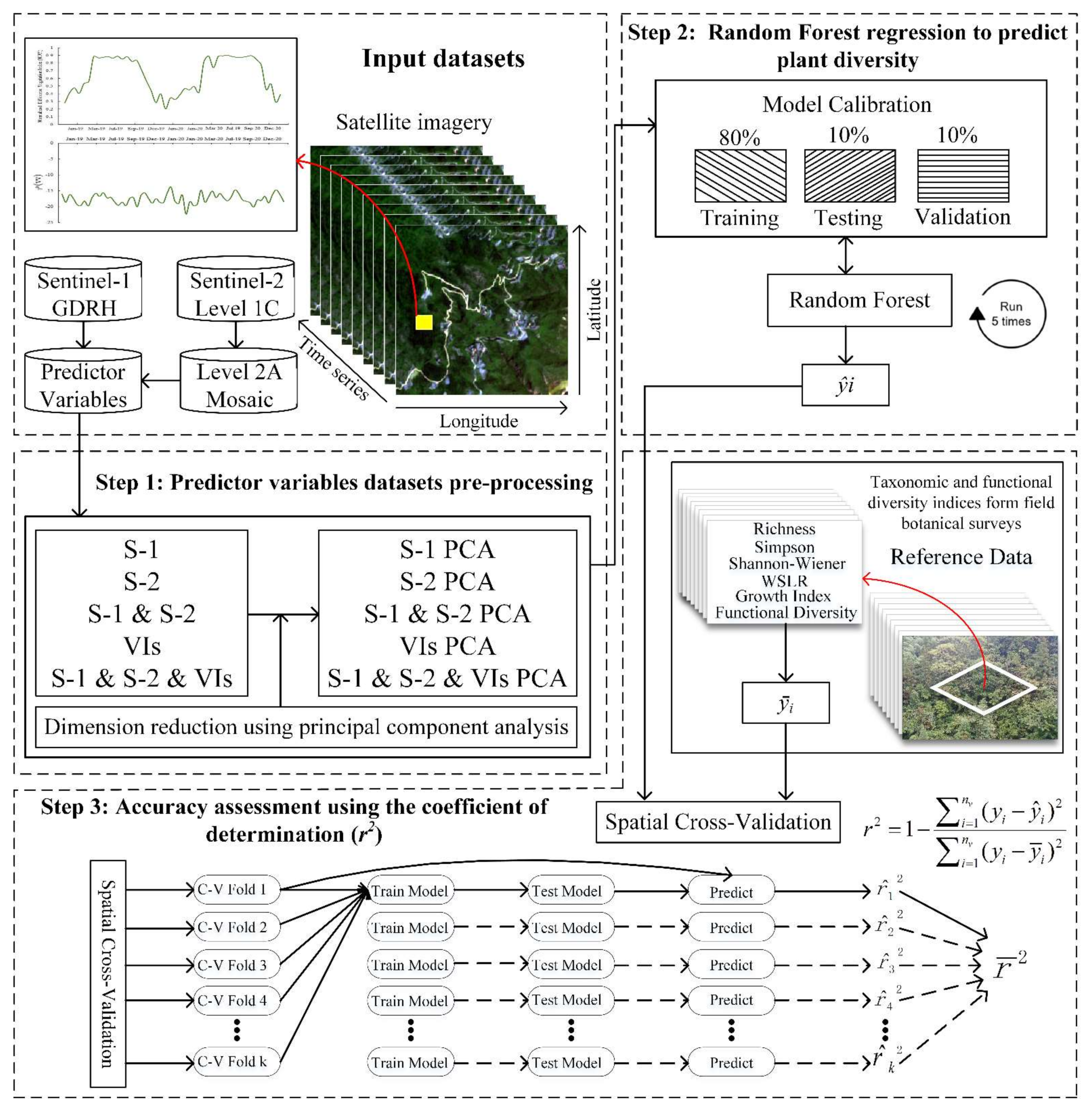
2.1. Overview

The time-series of S-1 and -2 data sets were used to estimate plant diversity indices in this study. The flowchart is shown in Figure 1. First, all of the imagery data sets were resampled to 10 m ground sampled distance and the principal component analysis (PCA) method was applied to retain the most discriminating bands to form 10 sets of predictor variables. Next, a random forest (RF) algorithm [64] was used to predict plant diversity based on the 10 sets of predictor variables. To represent the variability of the sample process, model calibration was repeated five times. Each time the training (80%), validation (10%) and testing (10%) datasets were randomly selected. Prediction results of each prediction were averaged. Finally, satellite imagery, along with field botanical survey data to calculate plant diversity indices (i.e., richness, Simpson, Shannon-Wiener, WSLR, growth index and texture diversity), was divided into training, validation and testing sets using spatial cross-validation [65]. The accuracy of the data was assessed by the coefficient of determination (ȓ2). All modeling and validation were performed in Python 3.70 [66]. RF [64] was run using the Scikit-learn python library.

2.2. Study Area

The study area is part of the Daba and Jingshan mountain ranges, located in northwestern Hubei Province of China, at 31°2′ to 32°6′N and 109°4′ to 112°9′E (Figure 2). The Jingshan and Daba mountain ranges serve as a watershed for the rivers between the Han River Basin and the Yangtze River Basin. The region lies in the transitional zone from the mid- to north-subtropical belts and covers an area of 15,290 km2 was considered as an experimental area. It is characterized by the following three forest vegetation types: evergreen broad-leaved forest, deciduous broad-leaved forest and evergreen-deciduous broad-leaved mixed forest. This intact subtropical forest ecosystem of the middle latitudes is very abundant in forest plant species [67]. The altitude of the study area ranges from 526 to 2741 m above sea level. The average rainfall of approximately 100–150 mm per month is caused by the influence of the southeast monsoon, while in the summer it can be approximately 150–200 mm per month [68]. The vertical zonal distribution of these forest vegetation types are distinct under the influence of topographic features [63]. The forests across the study area are comprised of about 72 dominant tree species. Spatial variations of precipitation, elevation, slope and aspect have led to spatial heterogeneity of the forest species composition and structure in natural or secondary subtropical evergreen broad-leaved species (e.g., Rhododendron hypoglaucum, Fagus lucida R. et W., Fagus engleriana S. and Cyclobalanopsis multinervis, et al.), temperate deciduous broad-leaved species (e.g., Betula albosinensis, Betula luminifera, Sinowilsonia henryi, Quercus aliena, Populus davidiana, Platycarya strobilacea and Sorbus folgneri, et al.) and coniferous species (e.g., Abies fargesii, Pinus massoniana, Cunninghamia lanceolata and Pinus armandii Fr., et al.) [3].

2.3. Datasets and Pre-Processing

2.3.1. Sentinel-2 Data Sets

A time-series of 51 S-2 images of Level 1C were captured from the United States Geological Survey website (earthexplorer.usgs.gov), corresponding to all available acquisition dates during two years of vegetation phenology (1 September 2018 and 31 August 2020) of this study area. The imagery datasets were geometrically calibrated, and the pixel values were converted into surface reflectance (SR) based on multi-sensor atmospheric correction and cloud screening algorithm [69]. Then, monthly mean SR values were calculated for each pixel of each quadrat. The bands at 10 and 20 m per pixel were used in the analyses. The characteristics of the imagery bands used for analysis are presented in Table 1. The 20-m bands were resampled to a 10-m grid based on the bilinear algorithm in the Sentinel Application Platform from the ESA. Next, these resampled bands were stacked up with the other 10-m bands into a temporary raster file on a geographic information system environment. The final time series of S-2 contain a total of 240 (24 dates × 10 bands) spectro-temporal feature pixels.

2.3.2. Sentinel-1 Data Sets

The time-series of S-1 imagery captured in an interferometric wide swath mode were used in this study. All 51 images were downloaded from the Alaska Satellite Facility website (vertex.daac.asf.alaska.edu), corresponding to the same temporal period as the time- series of S-2 data. The time-series of Sentinel-1 data were spatial calibrated, orthorectified and filtered based on a multi-scale spatiotemporal filter [70]. The window size of the spatiotemporal filter was 10 × 10 m. The vertical/vertical (VV) and vertical/horizontal (VH) polarizations were calculated, and the proportion VV/VH, where the first letter in each pair indicates emission and the second letter indicates reception. Similarly, monthly mean values were also calculated for the pixel of each quadrat. The final Sentinel-1 SITS contained a total of 72 (24 dates × 3 bands) temporal feature pixels.

2.4. Predictor Combined Variables

Accordingly, a series of predictor variables were generated using the S-1 and S-2 data. In addition, the predictor variables also considered six vegetation indices, i.e., Normalized Difference Vegetation Index (NDVI) [71], Enhanced Vegetation Index (EVI) [72], Land Surface Water Index (LSWI) [73], Normalized Difference Red-edge (NDVI705) [74], Normalized Difference Yellow Index (NDYI) [75] and Red-edge Position (REP) [76]. Calculating vegetation indices (VIs) based on different spectral parameters may improve the potentiality to separate different forest plant species [77], as VIs can decrease the spectral band signature variability of related to solar radiation, atmospheric conditions, scene lighting [8]. Therefore, the six VIs were also used to predict and map plant diversity in forests. Table 2 indicates an overview of 10 predictor combined variables. For five variables, the PCA method was used to retain the most discriminating information.

2.5. Reference Data

2.5.1. Field Surveys

Field surveys were accomplished in 448 quadrats from the subtropical evergreen-deciduous broad-leaved forest ranges from July to September 2019 when the plants were growing vigorously. Each quadrat was composed of one 100 m2 quadrat (10 m × 10 m), which was similar to one pixel of S-2 satellite imagery (Figure 3). Each plot was composed of 4 quadrats of 100 square meter area. The center of each quadrat corresponded to a Sentinel-2 pixel. Since the absolute geolocation is below 11 m~12 m at 95.5% confidence [42], a possible mis-registration between Sentinel-2 data and GPS can be observed for few pixels at some dates. The geographic coordinate of each quadrat center position was controlled with a handheld GPS unit (horizontal accuracy < 0.5 m, Garmin GPS72H, Taiwan, China).

2.5.2. Plant Diversity Indices

Forest plant species were visually identified and classified at the individual level, and the abundance of each plant species was evaluated by the number of individuals within each quadrat in the field survey. First, the taxonomic characteristics of forest plant species, including richness, Shannon-Wiener [78], Simpson [79], were applied to evaluate forest diversity indices. The Shannon-Wiener diversity index commonly measures spatial heterogeneity by considering the count of individuals, and the Simpson diversity index is a plant dominance index considering the extent of domination (or no domination) of a few species in the community [8].
(1)
Richness: Sq, explained as the total count of plant species in quadrat q.
(2)
Shannon-Wiener diversity index:
H q = S = 1 S q p q s l n p q s
where pqs is the relative abundance of the individual plant species s in quadrat q.
(3)
Simpson diversity index:
L q = 1 S = 1 S q p q s 2
Next, the functional attributes of subtropical forest ecosystems, including water and soil loss risk (WSLR), plant diseases and insect pests, as well as textural features [18], were also considered. These values reflect the species that are most likely to impact communities and ecosystems. The WSLR was measured for each sampling quadrat, based on its frequency. The values were: 0 value defined as “none”, 1 value defined as “little”, 2 value defined as “more” and 3 value defined as “plenty”. The total value score ranges from 0 to 3 for the WSLR index of the sampling quadrats. The growth index combines the amount of each plant disease and insect pest. The values were: 1 for “plant is growing well with no pests and diseases”, 0.5 for “plant is growing well but with some pests and diseases” and 0 for “plant is suffering from pests and diseases”. Texture of the sampling quadrats using textural features (i.e., number of patches, edge density and aggregation density) and plant height was derived from the Shannon-Wiener diversity index as follows:
T D q = ( j = 1 J q r q j ln r q j + j = 1 H q h q j l n h q j )
where rqj and hqj are the total value of the relative abundance and the height of the species j in quadrat q, respectively; Jq and Hq are the total value of textural features and height in quadrat q, respectively.
The taxonomic (Figure 4a–c) and functional diversities (Figure 4d–f) are shown for the distribution of six indices for all quadrats.

2.6. Random Forest Regression Analysis

The Random Forest (RF) regression algorithm [64] is an ensemble learning method using a bootstrapping based on the classification (discrete variables) and regression (continuous variables) trees (CART) analysis to predict a continuous response variable [80]. RF is robust against over-fitting, have high accuracy performance, and deal with large data sets well [64]. The RF regression was applied to establish a plant diversity prediction model by integrating the time-series of S-1 and S-2 parameters.
When training RF, the two hyperparameters have to be tuned in manually. As follows: ntree (number of trees) was set to its default (800), and mtry (i.e., number of predictor variables randomly sampled for each node) was set as the square root of the sum of input parameters.

2.7. Accuracy Assessment

The prediction accuracy of a plant diversity index value y was evaluated based on the coefficient of determination (r2) [8]:
r 2 = 1 i = 1 n v y i y i ^ 2 i = 1 n v y i y i ¯ 2
where nv is the number of validation samples based on botanical field survey, yi is the truth plant diversity value associated with the ith sample, ŷi is plant diversity value using RF algorithm predicted and ȳ is the average value of the sample from plant diversity values in field surveys.
The k-fold spatial cross-validation was applied to accurately evaluate the coefficient of determination (r2) [65]: the data were divided into k exactly equal-size, and the model was fitted on k–1 folds, and the r2 is calculated on the remaining hidden fold. This cross-validation process was calculated for all k folds: k = 1, 2, …, k. In the process, a 10-fold-grouped spatial cross-validation was executed, where the first eight folds contained 52 quadrats and the last two folds contained 60 quadrats. The error evaluation used the same folds, irrespective of the band features, pre-processing methods and plant diversity indices that were used.

3. Results

3.1. Model Performances

3.1.1. Prediction Accuracy Performances

Table 3 shows the results for predicting six plant diversity variables for different combined variables. In terms of plant diversity indices, two indices were predicted with an estimated ȓ2 > 0.60 and four indices with an ȓ2 > 0.50. Among them, the Simpson (ȓ2 = 0.67), Shannon-Wiener (ȓ2 = 0.64), texture diversity (ȓ2 = 0.56) and richness (ȓ2 = 0.53) indices were predicted quite well. However, the two other indices, WSLR (ȓ2 = 0.42) and growth index (ȓ2 = 0.36), provided less accurate predictions. In terms of remote sensing combined variables, S-1 & S-2 PCA and VIs PCA were found to be suitable for predicting taxonomic diversity (i.e., Simpson, Shannon-Wiener and richness indices), while S-1 & S-2 and S-1 & S-2 & VIs PCA were the best for predicting heterogeneity indices (i.e., growth, texture diversity and WSLR indices) (Table 3). However, the S-2 data alone gives better prediction accuracies than the S-1 data alone (e.g., S-W, ȓ2 of 0.32 using the S-2, and S-1 reached only 0.07). In addition, S-1 data can enhance the accuracy of the predicted heterogeneity indices by approximately 0.2 (e.g., TD, ȓ2 of 0.56 using the S-1 & S-2, and S-2 reached only 0.34; WSLR, ȓ2 of 0.33 using the S-1 & S-2 PCA, and S-2 PCA reached only 0.09; growth index, ȓ2 of 0.24 using the S-1 & S-2 PCA, and S-2 PCA reached only 0.07).
Again, using the PCA method does lead to improve the prediction accuracy (e.g., Simpson, ȓ2 of 0.67 using the S-1 & S-2 PCA, and S-1 & S-2 reached only 0.34). The VIs are less informative than the original set of imagery features and the prediction accuracy of plant diversity is lower except for Simpson (ȓ2 of 0.55; using the VIs, and S-2 reached only 0.29). However, combining VIs and S-1 & S-2 data set can promote the prediction performance slightly for some diversity indices, such as S-W (ȓ2 of 0.31 using the S-1 & S-2 & VIs, and S-1 & S-2 reached only 0.21) and WSLR (ȓ2 of 0.33 using the S-1 & S-2 & VIs, and S-1 & S-2 reached only 0.26). The prediction and evaluation for the representative result of each diversity index are shown in Figure 5, which was drawn according to the remote sensing combined variables data and diversity indices in the spatial cross-validation process. The different colormap indicates the standard deviation ( σ ^ r 2 ) of the k-fold spatial cross validation for prediction accuracy.

3.1.2. Mapping Performances

For the accuracy assessment of the maps, one typical sample area with different forest types and landcover was selected. Figure 6b–d shows an extract of the evaluation and prediction accuracies using remote sensing combined variables to predict the Simpson, Shannon-Wiener and texture diversity indices for this study area at the pixel level around the quadrat BGS-263. As for the mapping of Simpson and Shannon-Wiener, the overall accuracy was 79.4% and 73.5% respectively, while the texture diversity’s overall accuracy was merely 66.8%. Based on spatial cross-validation, Figure 6f–h also shows the confidence interval values (range from 0.01 to 0.4) corresponding to the diversity indices prediction results. From the evaluation and prediction information, the Simpson, Shannon-Wiener and texture diversity values (and its confidence interval values) indicate high spatial heterogeneity in the parcels around the quadrat BGS-263, corresponding to the subtropical evergreen-deciduous broad-leaved mixed forest plant species distribution that can be captured with a spatial resolution of 10 m per pixel. In addition, inter-pixel species distribution variability can also be captured in the adjacent fields.
The distribution of the predicted Simpson diversity indices the total area is described in Figure 7 for the most representative types of forests classified on the field surveys (i.e., evergreen broad-leaved forest, deciduous broad-leaved forest, shrubland, dense grass, impervious surface and cultivation land). These landcover types accounted for about 95% of the entire forests area of the plot BGS-263. The distribution of the Simpson diversity index of the several forest classes shows in (Figure 7). For example, evergreen broad-leaved forest (mainly range from 0.2 to 0.95, average value: 0.79), deciduous broad-leaved forest (mainly range from 0.14 to 0.73, average value: 0.52), shrubland (mainly range from 0.4 to 0.7, average value: 0.44) and dense grass (mainly range from 0.12 to 0.33, average value: 0.19) had the highest average values, while impervious surface (roads, building) and cultivation surface (farmland, orchard) had the lowest values (0.09 and 0.11, respectively). Evergreen and deciduous broad-leaved forests exhibit strong differences of spatial heterogeneity, with the former having lower diversity indices (i.e., Simpson, Figure 7) than the latter.

3.2. Large-Area Plant Diversity Indices Spatial Distribution

The map of the diversity indices (i.e., Simpson, Shannon-Wiener and Texture diversity) derived from the remote sensing combined variables prediction (Figure 8) highlights a clear difference in plant diversity spatial distribution for the large-area at the pixel level in the study area. The Simpson and texture diversity indices were higher in the whole study area, while the highest values of the Shannon-Wiener diversity indices were mainly concentrated in the southern area (i.e., Shennongjia region). Compared with the example from the Shannon-Wiener and texture diversity indices (Figure 8), the spatial distribution of Simpson index was less pronounced and differences occurred at area rather than pixel-level in the study area. The mapping of Simpson, Shannon-Wiener and texture diversity’s overall accuracy was 67.4%, 64.2% and 56.8% respectively. The Simpson index’s distribution indicates that the plant dominance community in the study area is also widely distributed. Based on S-1 & S-2 PCA and RF to predict Simpson index was stable, particularly in some terrain complex regions (Figure 8a). The strong differences in the prediction results were acquired between Shannon-Wiener and texture diversity by RF based on VIs PCA and S-1 & S-2.

4. Discussion

4.1. Influence of Input Data

4.1.1. Influence of Remote Sensing Combined Variables

Based on machine learning algorithm and combined remote sensed data sets, predictions performance of plant diversity was more precise for Simpson and Shannon-Wiener diversity indices than for plant species abundance (e.g., richness) [81]. The Simpson diversity index assigns more weight value to dominant species, while richness is only based on species presence or absence [8]. The presence of plant species in the understory (about 1% of cover) will affect species abundance but would be rarely directly captured by optical satellite sensors, while forests are more readily detectable. Therefore, the Simpson index (ȓ2 = 0.67) is more useful for monitoring and prediction using satellite sensors on a large geographical scale. Heterogeneity indices (i.e., WSLR, growth index and texture diversity) measures also showed an ȓ2 > 0.35, which is promising despite the fact that their links to remote sensing signals are not as clear as those for species diversity [9].
Because S-1 data (radar data) are not affected by clouds or shadows, this type of data can capture additional valuable information that can improve prediction accuracy in very cloudy situations [82]. In a study of the prediction of plant diversity, the radar S-1 imagery, however, was not shown to greatly enhance the accuracy of plant diversity in grasslands [8]. This may have occurred because S-1 is insensitive to structural information in grasslands. The S-1 data, in the present study, was found to improve the prediction accuracy of forest plant diversity by approximately 0.2. Indeed, the integration of the time series of S-1 and S-2 data enhanced the prediction accuracy for several plant diversity indices, e.g., Simpson diversity index (ȓ2 of 0.67 using RF algorithm and S-1 & S-2 PCA) and texture diversity index (ȓ2 of 0.56 using RF algorithm and S-1 & S-2). Although S-1 data were distinctly expected to be insensitive to the composition of a plant community, it could have provided valuable information about plant geometric structure that could be connected to heterogeneity in the species present in an area [83]. Meanwhile, S-2 multispectral reflectivity data are influenced by chemical properties of the observed environment [33]. Therefore, integrating the strengths of S-1 and S-2 data sets have positive influence on the forest’s plant diversity prediction and mapping accuracy.
The full set of time-series data with irregular acquisition dates between diverse Sentinel imagery was processed using linear interpolation in this study [8]. This brought plenty of band information (Table 2) that can make the random forest algorithm parameter tuning more complex. The RF regression method was used to predict plant diversity in forests, and this method resulted promote the accuracy of prediction (ȓ2) by approximately 0.2 (Shannon-Wiener diversity index, ȓ2 of 0.64 using S-1 & S-2 PCA, but S-1 & S-2 reached only 0.47). The results indicate that it is appropriate to ignore the redundant features of the time series of Sentinel imagery when performing feature dimension reduction and investigation to capture valuable information from the data [45].

4.1.2. Influence of Different Features

Generally, clouds and shadows are unavoidably appearing on any spectral imagery having a large-scale extent, particularly during the period of plant growth (May–September). Hence, the image acquisition dates have a large influence the prediction accuracy of plant diversity indices. The 24 single-date S-1 and -2 images and 20 single-feature images using RF methods to predict the Simpson index are shown in Figure 9a. The ȓ2 was lower and varied significantly when using the 24 single-date S-1 and -2 imagery data. Accuracy of prediction was the lowest during periods of plant dormancy (December 2018 to February 2019, December 2019 to February 2020), while it was the highest during the growing periods (September to October 2018, March to August 2019 and June to August 2020). Specifically, maximum accuracy was ȓ2 = 0.46 on August 2019 (Figure 10a), while minimum accuracy ȓ2 did not surpass 0.1 on January 2020 (Figure 10d).
In contrast with the acquisition dates, each band data had a slight effect on the variation in accuracy (ȓ2), see Figure 9b. The accuracy of prediction was the lowest in the SWIR2 band (ȓ2 = 0.09), while it was the highest in the R band (ȓ2 = 0.43) (Figure 10b) and NIR1 band (ȓ2 = 0.37) (Figure 10e). However, B, G, RE1, RE2, RE3, NIR2 and SWIR1 bands were similar accuracies of prediction, ranging from 0.14 to 0.36. The radar data VV, VH and VV/VH to predict plant diversity accuracies ranged from 0.18 to 0.24. By inspecting the input features to the prediction accuracy, the VIs were shown to be far more reliable in prediction than the original radar and optical bands, particularly the NDVI705 and NDYI. This demonstrates that carefully selected VIs can also predict plant diversity, see Figure 9b. Accuracy was the lowest in the LSWI (ȓ2 = 0.21) (Figure 10f), while it was the highest in the NDVI705 (ȓ2 = 0.49) (Figure 10c). However, NDVI, EVI, NDYI and REP had similar accuracies, ranging from 0.24 to 0.45. The result indicates that with the relatively rich spectral band information, S-2 imagery has great advantages in predicting and mapping plant diversity in forests.
The summer/early fall season (May–September) was the most informative period for delineating areas of plant diversity (Figure 11). Previously, remote sensing-based researches have also shown that this season is vital for the study of characteristics such as plant phenology [50] and vegetation cover [84]. This period is also regarded as “the optimal moment” because precipitation falls quickly and abundantly within weeks [45], and forest plant growth reaches the peak [85]. Our results indicate that capturing changes in forest phenology with remote sensing time-series data can help improve prediction accuracy of plant diversity when spatial resolutions are not reached predicting demand. Some studies indicate a higher correlation between the band features and α diversity index (e.g., Shannon-Wiener) for simulated spectral imagery above 2 m per pixel [86]. However, these studies used data of only a single date and captured little key information for plant phenology. Although our prediction accuracy was inferior to these studies which predicted the Simpson diversity index based on airborne LiDAR and hyperspectral data [3], it can reflect plant diversity temporal variation in two vegetation phenology periods (two years). Therefore, with the increasing availability of higher spatial-temporal resolution imagery (e.g., Sentinel), these will provide a new paradigm for seasonal variation monitoring of plant diversity in high vegetation areas [87].
Feilhauer et al. (2013) indicated that the hyperspectral imagery of satellites is the most crucial feature that can be used to successfully estimate the plant variation in forests [88]. However, the results captured from the entire spectral information contradicted our data captured with Sentinel imagery data where the accuracies were accomplished using only the SWIR and NIR spectral bands. The studies indicated that spectral bands, such as RE, NIR and SWIR, had a clear influence on the plant diversity evaluation and prediction. Nevertheless, using only some VIs (NDYI and NDVI705) also acquired a good result. This may be because we carefully considered each VIs characteristics over all dates in the time-series images, which could have “smoothed” the difference of spectral reflectance during the plant phenology in the subtropical forest.

4.2. Spatial Heterogeneity of Result Analysis for Plant Diversity Mapping

The spatial heterogeneity of plant diversity indices of the studied subtropical evergreen-deciduous broad-leaved mixed forest is shown in Figure 8. The large-area map emphasizes the forest intra-parcel heterogeneity in terms of plant diversity, highlighting the restrictions of predicting biodiversity indices at the field scale. This type of map can also be applied to evaluate the relationships between environmental factors and plant diversity at a pixel level [89]. The prediction results associated with the large-scale confidence intervals captured in the satellite imagery can be defined by regional topographical conditions [63]. Spectral-temporal features were found to do not correspond to input data sets from which learns to identify forest types, resulting in inaccurate predictions, especially in the edges of the parcels (Figure 6). First of all, the edges of the parcels could amount to mixed pixels and thus display indeterminate values. Second, evergreen-deciduous broad-leaved mixed forests are usually included in the one pixel. The one lesson is that the field quadrat size should match as much as possible the remote sensor’s spatial resolution. These results also indicate that the remote sensing-based assessment of forest plant diversity should be carried out at the field quadrat level and not at the pixel level. Similarly, examining the confidence intervals of prediction diversity indices could thus indicate the dependability of mapping accuracy at the pixel level [90].
Previous studies have rarely considered the spatial heterogeneity of plant diversity in forests [44], although it can have a significant impact on the evaluated prediction accuracy of plant diversity. Figure 7 shows the decreasing average of the predicted Simpson diversity index values from the evergreen broad-leaved forest and shrubland. The results are consistent with the long-term no-felling and low-level forest management activities that are designed to maintain plant diversity at a higher level. However, dense grass present Simpson diversity index values that are similar to the values of cultivated land. This is because dense grass will restrict tillage, while cultivated areas do not. This pattern can also be defined by the true situation that the number of remote sensing imagery visual interpretation with dense grass are often lower than the field survey values (it ought to be identified as “cultivated land” instead). The complexity of landcover types clearly shows that using remotely sensed data sets to map plant diversity need to combine and refer to the botanical field surveys assessment across the subtropical mountainous forests. These large-area plant diversity maps of spatially explicit, wall-to-wall, precise and frequently updated information can provide reasonable assessments of spatial heterogeneity and diversity distribution across wide areas.

5. Conclusions

The introduced S-1 and S-2 workflow for forest plant diversity is cost-efficient and scalable. The workflow was already successfully applied in a subtropical evergreen-deciduous broad-leaved mixed forest. Compared with traditional field surveys designed to forest plant species, the workflow is proposed for mapping plant diversity based on the time-series of S-1 and S-2 and machine learning algorithm, and has two main advantages. First, the workflow considered the combined remote sensing data variability in the forest plant diversity. In terms of remote sensing combined variables, S-1 & S-2 PCA was found to be suitable for predicting taxonomic diversity, while S-1 & S-2 was the best for predicting growth and texture diversity indices. Second, the workflow considered the spatial heterogeneity of plant distribution, which is unordered, and used spatial and temporal remote sensing data to predict plant diversity maps. Results show that plant diversity indices spatial heterogeneity (and its related confidence values) were captured in the forest parcels, consistent with the spatial heterogeneity of plant distribution that was obtained with a 10 m resolution. In addition, the use of radar data can increase the accuracy of prediction (ȓ2) by approximately 0.2. Imagery sources and time-series data were considered when evaluating the error of the accuracy of the predicted plant diversity.
The contribution of this study is that the time-series of S-1 and S-2 data based on forest vegetation phenology differences can be used to map plant diversity. This study also illustrates that the potential of the time-series of S-1 and S-2 and plant phenology for the mapping plant diversity indices in forests. It could therefore help promote forest ecosystem and resource conservation activities in the forestry sector that depend on timely and accurate spatial distribution of forest plant diversity.

Author Contributions

Conceptualization and methodology, Q.Y., L.W. and F.L.; software, Q.Y.; validation, L.W. and J.H.; formal analysis, Q.Y. and L.L.; investigation, Q.Y., L.L. and Y.L.; resources, Q.Y., L.W. and F.L.; data curation, Q.Y., L.W., Y.D. and F.L.; writing—original draft preparation, Q.Y. and L.W.; writing—review and editing, Q.Y., L.W., J.H., Y.D. and F.L.; visualization, Q.Y.; supervision, L.W., J.H. and F.L.; project administration, L.W.; funding acquisition, L.W. and F.L. All authors have read and agreed to the published version of the manuscript.

Funding

This research was founded by the National Natural Science Foundation of China (Grant No. 51809250) and Hubei Provincial Natural Science Foundation for Innovation Groups (Grant No. 2019CFA019).

Data Availability Statement

Not applicable.

Acknowledgments

We thank to Tingting Li and Zhengxiang Wang (Hubei University) for providing valuable plants distribution information and designing of the sampling plots. We also appreciate the help of Yuyang Xu, Bangjun Lin, Hehe Zhang, Ling Li, Ze Li, Rongyou Chen; Wei Xiong and Wenjuan Zhang; Ruyue Ma during fieldwork. The authors would also like to thank the reviewers and the handling editor whose comments and suggestions improved this paper.

Conflicts of Interest

The authors declare that they have no known commercial or financial competing interest that represents a conflict of interest in this paper.

References

  1. Schäfer, E.; Heiskanen, J.; Heikinheimo, V.; Pellikka, P. Mapping tree species diversity of a tropical montane forest by unsupervised clustering of airborne imaging spectroscopy data. Ecol. Indic. 2016, 64, 49–58. [Google Scholar] [CrossRef]
  2. Lausch, A.; Erasmi, S.; King, D.; Magdon, P.; Heurich, M. Understanding Forest Health with Remote Sensing—Part I—A Review of Spectral Traits, Processes and Remote-Sensing Characteristics. Remote Sens. 2016, 8, 121029. [Google Scholar] [CrossRef] [Green Version]
  3. Zhao, Y.; Zeng, Y.; Zheng, Z.; Dong, W.; Zhao, D.; Wu, B.; Zhao, Q. Forest species diversity mapping using airborne LiDAR and hyperspectral data in a subtropical forest in China. Remote Sens. Environ. 2018, 213, 104–114. [Google Scholar] [CrossRef]
  4. Harrison, P.A.; Berry, P.M.; Simpson, G.; Haslett, J.R.; Blicharska, M.; Bucur, M.; Dunford, R.; Egoh, B.; Garcia-Llorente, M.; Geamănă, N.; et al. Linkages between biodiversity attributes and ecosystem services: A systematic review. Ecosyst. Serv. 2014, 9, 191–203. [Google Scholar] [CrossRef] [Green Version]
  5. Torresani, M.; Rocchini, D.; Sonnenschein, R.; Zebisch, M.; Marcantonio, M.; Ricotta, C.; Tonon, G. Estimating tree species diversity from space in an alpine conifer forest: The Rao’s Q diversity index meets the spectral variation hypothesis. Ecol. Inform. 2019, 52, 26–34. [Google Scholar] [CrossRef] [Green Version]
  6. Gholizadeh, H.; Gamon, J.A.; Zygielbaum, A.I.; Wang, R.; Schweiger, A.K.; Cavender-Bares, J. Remote sensing of biodiversity: Soil correction and data dimension reduction methods improve assessment of α-diversity (species richness) in prairie ecosystems. Remote Sens. Environ. 2018, 206, 240–253. [Google Scholar] [CrossRef]
  7. Vihervaara, P.; Auvinen, A.-P.; Mononen, L.; Törmä, M.; Ahlroth, P.; Anttila, S.; Böttcher, K.; Forsius, M.; Heino, J.; Heliölä, J.; et al. How Essential Biodiversity Variables and remote sensing can help national biodiversity monitoring. Glob. Ecol. Conserv. 2017, 10, 43–59. [Google Scholar] [CrossRef]
  8. Fauvel, M.; Lopes, M.; Dubo, T.; Rivers-Moore, J.; Frison, P.-L.; Gross, N.; Ouin, A. Prediction of plant diversity in grasslands using Sentinel-1 and -2 satellite image time series. Remote Sens. Environ. 2020, 237. [Google Scholar] [CrossRef]
  9. Hamrouni, Y.; Paillassa, E.; Chéret, V.; Monteil, C.; Sheeren, D. From local to global: A transfer learning-based approach for mapping poplar plantations at national scale using Sentinel-2. ISPRS J. Photogramm. Remote Sens. 2021, 171, 76–100. [Google Scholar] [CrossRef]
  10. Keenan, R.J. Climate change impacts and adaptation in forest management: A review. Ann. For. Sci. 2015, 72, 145–167. [Google Scholar] [CrossRef] [Green Version]
  11. Wallis, C.I.B.; Paulsch, D.; Zeilinger, J.; Silva, B.; Curatola Fernández, G.F.; Brandl, R.; Farwig, N.; Bendix, J. Contrasting performance of Lidar and optical texture models in predicting avian diversity in a tropical mountain forest. Remote Sens. Environ. 2016, 174, 223–232. [Google Scholar] [CrossRef]
  12. Zhang, H.; Yang, Q.; Zhou, D.; Xu, W.; Gao, J.; Wang, Z. How evergreen and deciduous trees coexist during secondary forest succession: Insights into forest restoration mechanisms in Chinese subtropical forest. Glob. Ecol. Conserv. 2021, 25, e01418. [Google Scholar] [CrossRef]
  13. Tang, H.; Armston, J.; Hancock, S.; Marselis, S.; Goetz, S.; Dubayah, R. Characterizing global forest canopy cover distribution using spaceborne lidar. Remote Sens. Environ. 2019, 231, 111262. [Google Scholar] [CrossRef]
  14. Madonsela, S.; Cho, M.A.; Ramoelo, A.; Mutanga, O. Remote sensing of species diversity using Landsat 8 spectral variables. ISPRS J. Photogramm. Remote Sens. 2017, 133, 116–127. [Google Scholar] [CrossRef] [Green Version]
  15. Arekhi, M.; Yilmaz, O.Y.; Yilmaz, H.; Akyuz, Y.F. Can tree species diversity be assessed with Landsat data in a temperate forest? Environ. Monit. Assess. 2017, 189, 586. [Google Scholar] [CrossRef]
  16. Randin, C.F.; Ashcroft, M.B.; Bolliger, J.; Cavender-Bares, J.; Coops, N.C.; Dullinger, S.; Dirnböck, T.; Eckert, S.; Ellis, E.; Fernández, N.; et al. Monitoring biodiversity in the Anthropocene using remote sensing in species distribution models. Remote Sens. Environ. 2020, 239, 111626. [Google Scholar] [CrossRef]
  17. Díaz, S.; Cabido, M. Vive la différence: Plant functional diversity matters to ecosystem processes. Trends Ecol. Evol. 2001, 16, 646–655. [Google Scholar] [CrossRef]
  18. Li, Y.; Feng, G.; Tewolde, H.; Yang, M.; Zhang, F. Soil, biochar, and nitrogen loss to runoff from loess soil amended with biochar under simulated rainfall. J. Hydrol. 2020, 591, 125318. [Google Scholar] [CrossRef]
  19. Cavender-Bares, J.; Gamon, J.A.; Hobbie, S.E.; Madritch, M.D.; Meireles, J.E.; Schweiger, A.K.; Townsend, P.A. Harnessing plant spectra to integrate the biodiversity sciences across biological and spatial scales. Am. J. Bot. 2017, 104, 966–969. [Google Scholar] [CrossRef] [PubMed] [Green Version]
  20. Rocchini, D.; Balkenhol, N.; Carter, G.A.; Foody, G.M.; Gillespie, T.W.; He, K.S.; Kark, S.; Levin, N.; Lucas, K.; Luoto, M.; et al. Remotely sensed spectral heterogeneity as a proxy of species diversity: Recent advances and open challenges. Ecol. Inform. 2010, 5, 318–329. [Google Scholar] [CrossRef]
  21. Mura, M.; McRoberts, R.E.; Chirici, G.; Marchetti, M. Estimating and mapping forest structural diversity using airborne laser scanning data. Remote Sens. Environ. 2015, 170, 133–142. [Google Scholar] [CrossRef]
  22. Warren, S.D.; Alt, M.; Olson, K.D.; Irl, S.D.H.; Steinbauer, M.J.; Jentsch, A. The relationship between the spectral diversity of satellite imagery, habitat heterogeneity, and plant species richness. Ecol. Inform. 2014, 24, 160–168. [Google Scholar] [CrossRef]
  23. Rocchini, D.; Boyd, D.S.; Féret, J.B.; Foody, G.M.; He, K.S.; Lausch, A.; Nagendra, H.; Wegmann, M.; Pettorelli, N.; Skidmore, A.; et al. Satellite remote sensing to monitor species diversity: Potential and pitfalls. Remote Sens. Ecol. Conserv. 2015, 2, 25–36. [Google Scholar] [CrossRef]
  24. Ceballos, A.; Hernández, J.; Corvalán, P.; Galleguillos, M. Comparison of Airborne LiDAR and Satellite Hyperspectral Remote Sensing to Estimate Vascular Plant Richness in Deciduous Mediterranean Forests of Central Chile. Remote Sens. 2015, 7, 2692–2714. [Google Scholar] [CrossRef] [Green Version]
  25. Turner, W. Sensing biodiversity. Science 2014, 346, 301–302. [Google Scholar] [CrossRef]
  26. Belmonte, A.; Sankey, T.; Biederman, J.A.; Bradford, J.; Goetz, S.J.; Kolb, T.; Woolley, T.; Horning, N.; Bohlman, S. UAV-derived estimates of forest structure to inform ponderosa pine forest restoration. Remote Sens. Ecol. Conserv. 2019, 6, 181–197. [Google Scholar] [CrossRef]
  27. Dandois, J.; Olano, M.; Ellis, E. Optimal Altitude, Overlap, and Weather Conditions for Computer Vision UAV Estimates of Forest Structure. Remote Sens. 2015, 7, 13895–13920. [Google Scholar] [CrossRef] [Green Version]
  28. Simonson, W.D.; Allen, H.D.; Coomes, D.A.; Tatem, A. Applications of airborne lidar for the assessment of animal species diversity. Methods Ecol. Evol. 2014, 5, 719–729. [Google Scholar] [CrossRef]
  29. Dash, J.P.; Watt, M.S.; Pearse, G.D.; Heaphy, M.; Dungey, H.S. Assessing very high resolution UAV imagery for monitoring forest health during a simulated disease outbreak. ISPRS J. Photogramm. Remote Sens. 2017, 131, 1–14. [Google Scholar] [CrossRef]
  30. Carrasco, L.; Giam, X.; Papeş, M.; Sheldon, K. Metrics of Lidar-Derived 3D Vegetation Structure Reveal Contrasting Effects of Horizontal and Vertical Forest Heterogeneity on Bird Species Richness. Remote Sens. 2019, 11, 743. [Google Scholar] [CrossRef] [Green Version]
  31. Leutner, B.F.; Reineking, B.; Müller, J.; Bachmann, M.; Beierkuhnlein, C.; Dech, S.; Wegmann, M. Modelling Forest α-Diversity and Floristic Composition—On the Added Value of LiDAR plus Hyperspectral Remote Sensing. Remote Sens. 2012, 4, 2818–2845. [Google Scholar] [CrossRef] [Green Version]
  32. Liu, Y.; Gong, W.; Xing, Y.; Hu, X.; Gong, J. Estimation of the forest stand mean height and aboveground biomass in Northeast China using SAR Sentinel-1B, multispectral Sentinel-2A, and DEM imagery. ISPRS J. Photogramm. Remote Sens. 2019, 151, 277–289. [Google Scholar] [CrossRef]
  33. Adrian, J.; Sagan, V.; Maimaitijiang, M. Sentinel SAR-optical fusion for crop type mapping using deep learning and Google Earth Engine. ISPRS J. Photogramm. Remote Sens. 2021, 175, 215–235. [Google Scholar] [CrossRef]
  34. Hauser, L.T.; Féret, J.-B.; An Binh, N.; van der Windt, N.; Sil, Â.F.; Timmermans, J.; Soudzilovskaia, N.A.; van Bodegom, P.M. Towards scalable estimation of plant functional diversity from Sentinel-2: In-situ validation in a heterogeneous (semi-)natural landscape. Remote Sens. Environ. 2021, 262, 112505. [Google Scholar] [CrossRef]
  35. Guerschman, J.P.; Hill, M.J.; Leys, J.; Heidenreich, S. Vegetation cover dependence on accumulated antecedent precipitation in Australia: Relationships with photosynthetic and non-photosynthetic vegetation fractions. Remote Sens. Environ. 2020, 240, 111670. [Google Scholar] [CrossRef]
  36. Ge, J.; Meng, B.; Liang, T.; Feng, Q.; Gao, J.; Yang, S.; Huang, X.; Xie, H. Modeling alpine grassland cover based on MODIS data and support vector machine regression in the headwater region of the Huanghe River, China. Remote Sens. Environ. 2018, 218, 162–173. [Google Scholar] [CrossRef]
  37. Rocchini, D. Effects of spatial and spectral resolution in estimating ecosystem α-diversity by satellite imagery. Remote Sens. Environ. 2007, 111, 423–434. [Google Scholar] [CrossRef]
  38. Wang, R.; Gamon, J.A. Remote sensing of terrestrial plant biodiversity. Remote Sens. Environ. 2019, 231, 111218. [Google Scholar] [CrossRef]
  39. Wyniawskyj, N.S.; Napiorkowska, M.; Petit, D.; Podder, P.; Marti, P. Forest Monitoring in Guatemala Using Satellite Imagery and Deep Learning. In Proceedings of the IGARSS 2019—2019 IEEE International Geoscience and Remote Sensing Symposium, Yokohama, Japan, 28 July–2 August 2019; pp. 6598–6601. [Google Scholar]
  40. Shin, P.; Sankey, T.; Moore, M.; Thode, A. Evaluating Unmanned Aerial Vehicle Images for Estimating Forest Canopy Fuels in a Ponderosa Pine Stand. Remote Sens. 2018, 10, 1266. [Google Scholar] [CrossRef] [Green Version]
  41. Yuan, H.; Yang, G.; Li, C.; Wang, Y.; Liu, J.; Yu, H.; Feng, H.; Xu, B.; Zhao, X.; Yang, X. Retrieving Soybean Leaf Area Index from Unmanned Aerial Vehicle Hyperspectral Remote Sensing: Analysis of RF, ANN, and SVM Regression Models. Remote Sens. 2017, 9, 309. [Google Scholar] [CrossRef] [Green Version]
  42. European Space Agency (E.S.A.). Copernicus Missions. 2021. Available online: https://sentinel.esa.int/web/sentinel/missions/sentinel-1 (accessed on 15 May 2021).
  43. Defourny, P.; Bontemps, S.; Bellemans, N.; Cara, C.; Dedieu, G.; Guzzonato, E.; Hagolle, O.; Inglada, J.; Nicola, L.; Rabaute, T.; et al. Near real-time agriculture monitoring at national scale at parcel resolution: Performance assessment of the Sen2-Agri automated system in various cropping systems around the world. Remote Sens. Environ. 2019, 221, 551–568. [Google Scholar] [CrossRef]
  44. You, N.; Dong, J. Examining earliest identifiable timing of crops using all available Sentinel 1/2 imagery and Google Earth Engine. ISPRS J. Photogramm. Remote Sens. 2020, 161, 109–123. [Google Scholar] [CrossRef]
  45. Rapinel, S.; Mony, C.; Lecoq, L.; Clément, B.; Thomas, A.; Hubert-Moy, L. Evaluation of Sentinel-2 time-series for mapping floodplain grassland plant communities. Remote Sens. Environ. 2019, 223, 115–129. [Google Scholar] [CrossRef]
  46. Mura, M.; Bottalico, F.; Giannetti, F.; Bertani, R.; Giannini, R.; Mancini, M.; Orlandini, S.; Travaglini, D.; Chirici, G. Exploiting the capabilities of the Sentinel-2 multi spectral instrument for predicting growing stock volume in forest ecosystems. Int. J. Appl. Earth Obs. Geoinf. 2018, 66, 126–134. [Google Scholar] [CrossRef]
  47. Van Passel, J.; De Keersmaecker, W.; Somers, B. Monitoring Woody Cover Dynamics in Tropical Dry Forest Ecosystems Using Sentinel-2 Satellite Imagery. Remote Sens. 2020, 12, 1276. [Google Scholar] [CrossRef] [Green Version]
  48. Persson, M.; Lindberg, E.; Reese, H. Tree Species Classification with Multi-Temporal Sentinel-2 Data. Remote Sens. 2018, 10, 1794. [Google Scholar] [CrossRef] [Green Version]
  49. Waser, L.T.; Rüetschi, M.; Psomas, A.; Small, D.; Rehush, N. Mapping dominant leaf type based on combined Sentinel-1/-2 data—Challenges for mountainous countries. ISPRS J. Photogramm. Remote Sens. 2021, 180, 209–226. [Google Scholar] [CrossRef]
  50. Tian, F.; Cai, Z.; Jin, H.; Hufkens, K.; Scheifinger, H.; Tagesson, T.; Smets, B.; Van Hoolst, R.; Bonte, K.; Ivits, E.; et al. Calibrating vegetation phenology from Sentinel-2 using eddy covariance, PhenoCam, and PEP725 networks across Europe. Remote Sens. Environ. 2021, 260, 112456. [Google Scholar] [CrossRef]
  51. Forkuor, G.; Benewinde Zoungrana, J.-B.; Dimobe, K.; Ouattara, B.; Vadrevu, K.P.; Tondoh, J.E. Above-ground biomass mapping in West African dryland forest using Sentinel-1 and 2 datasets—A case study. Remote Sens. Environ. 2020, 236, 111496. [Google Scholar] [CrossRef]
  52. Chen, L.; Wang, Y.; Ren, C.; Zhang, B.; Wang, Z. Optimal Combination of Predictors and Algorithms for Forest Above-Ground Biomass Mapping from Sentinel and SRTM Data. Remote Sens. 2019, 11, 414. [Google Scholar] [CrossRef] [Green Version]
  53. Hemmerling, J.; Pflugmacher, D.; Hostert, P. Mapping temperate forest tree species using dense Sentinel-2 time series. Remote Sens. Environ. 2021, 267, 112743. [Google Scholar] [CrossRef]
  54. Rüetschi, M.; Schaepman, M.; Small, D. Using Multitemporal Sentinel-1 C-band Backscatter to Monitor Phenology and Classify Deciduous and Coniferous Forests in Northern Switzerland. Remote Sens. 2017, 10, 55. [Google Scholar] [CrossRef] [Green Version]
  55. Fassnacht, F.E.; Latifi, H.; Stereńczak, K.; Modzelewska, A.; Lefsky, M.; Waser, L.T.; Straub, C.; Ghosh, A. Review of studies on tree species classification from remotely sensed data. Remote Sens. Environ. 2016, 186, 64–87. [Google Scholar] [CrossRef]
  56. Zhao, F.; Sun, R.; Zhong, L.; Meng, R.; Huang, C.; Zeng, X.; Wang, M.; Li, Y.; Wang, Z. Monthly mapping of forest harvesting using dense time series Sentinel-1 SAR imagery and deep learning. Remote Sens. Environ. 2022, 269, 112822. [Google Scholar] [CrossRef]
  57. Reiche, J.; Lucas, R.; Mitchell, A.L.; Verbesselt, J.; Hoekman, D.H.; Haarpaintner, J.; Kellndorfer, J.M.; Rosenqvist, A.; Lehmann, E.A.; Woodcock, C.E.J.N.C.C. Combining satellite data for better tropical forest monitoring. Nat. Clim. Chang. 2016, 6, 120–122. [Google Scholar] [CrossRef]
  58. Lopes, M.; Frison, P.L.; Durant, S.M.; Schulte to Bühne, H.; Ipavec, A.; Lapeyre, V.; Pettorelli, N.; Horning, N. Combining optical and radar satellite image time series to map natural vegetation: Savannas as an example. Remote Sens. Ecol. Conserv. 2020, 6, 316–326. [Google Scholar] [CrossRef]
  59. Mercier, A.; Betbeder, J.; Denize, J.; Roger, J.L.; Spicher, F.; Lacoux, J.; Roger, D.; Baudry, J.; Hubert-Moy, L. Estimating crop parameters using Sentinel-1 and 2 datasets and geospatial field data. Data Brief. 2021, 38, 107408. [Google Scholar] [CrossRef]
  60. Schulz, D.; Yin, H.; Tischbein, B.; Verleysdonk, S.; Adamou, R.; Kumar, N. Land use mapping using Sentinel-1 and Sentinel-2 time series in a heterogeneous landscape in Niger, Sahel. ISPRS J. Photogramm. Remote Sens. 2021, 178, 97–111. [Google Scholar] [CrossRef]
  61. Bhattarai, R.; Rahimzadeh-Bajgiran, P.; Weiskittel, A.; Meneghini, A.; MacLean, D.A. Spruce budworm tree host species distribution and abundance mapping using multi-temporal Sentinel-1 and Sentinel-2 satellite imagery. ISPRS J. Photogramm. Remote Sens. 2021, 172, 28–40. [Google Scholar] [CrossRef]
  62. Erinjery, J.J.; Singh, M.; Kent, R. Mapping and assessment of vegetation types in the tropical rainforests of the Western Ghats using multispectral Sentinel-2 and SAR Sentinel-1 satellite imagery. Remote Sens. Environ. 2018, 216, 345–354. [Google Scholar] [CrossRef]
  63. Yang, Q.; Zhang, H.; Wang, L.; Ling, F.; Wang, Z.; Li, T.; Huang, J. Topography and soil content contribute to plant community composition and structure in subtropical evergreen-deciduous broadleaved mixed forests. Plant Divers. 2021. [Google Scholar] [CrossRef]
  64. Breiman, L. Random forests. Mach. Learn. 2001, 45, 5–32. [Google Scholar] [CrossRef] [Green Version]
  65. Le Rest, K.; Pinaud, D.; Monestiez, P.; Chadoeuf, J.; Bretagnolle, V. Spatial leave-one-out cross-validation for variable selection in the presence of spatial autocorrelation. Glob. Ecol. Biogeogr. 2014, 23, 811–820. [Google Scholar] [CrossRef] [Green Version]
  66. R Core Team. R: A Language and Environment for Statistical Computing; R Foundation for Statistical Computing: Vienna, Austria, 2021; Available online: https://www.R-project.org/ (accessed on 14 May 2021).
  67. Yang, Q.; Li, T.; Wang, Z.; Xu, Y.; Zhang, H.; Li, L. Spatial scale analysis of the species diversity and distribution of rare and endangered plants in northwest Hubei, China. Plant Sci. J. 2019, 37, 464–473. [Google Scholar]
  68. Zeng, Y.; Schaepman, M.; Wu, B.; Clevers, J.; Bregt, A. Scaling-based forest structural change detection using an inverted geometric-optical model in the Three Gorges region of China. Remote Sens. Environ. 2008, 112, 4261–4271. [Google Scholar] [CrossRef]
  69. Hagolle, O.; Huc, M.; Villa Pascual, D.; Dedieu, G. A Multi-Temporal and Multi-Spectral Method to Estimate Aerosol Optical Thickness over Land, for the Atmospheric Correction of FormoSat-2, LandSat, VENμS and Sentinel-2 Images. Remote Sens. 2015, 7, 2668–2691. [Google Scholar] [CrossRef] [Green Version]
  70. Quegan, S.; Yu, J.J. Filtering of Multichannel SAR Images. IEEE Trans. Geosci. Remote Sens. 2001, 39, 2373–2380. [Google Scholar] [CrossRef]
  71. Matton, N.; Waldner, F.; Valero, S.; Morin, D.; Inglada, J.; Arias, M.; Bontemps, S.; Koetz, B.; Defourny, P. Red and photographic infrared linear combinations for monitoring vegetation. Remote Sens. Environ. 1979, 8, 127–150. [Google Scholar]
  72. Huete, A.R.; Liu, H.Q.; Batchily, K.; Leeuwen, W.V. A Comparison of Vegetation Indices over a Global Set of TM Images for EOS-MODIS. Remote Sens. Environ. 1997, 59, 440–451. [Google Scholar] [CrossRef]
  73. Xiao, X.; Hollinger, D.; Aber, J.; Goltz, M.; Davidson, E.A.; Zhang, Q.; Moore, B. Satellite-based modeling of gross primary production in an evergreen needleleaf forest. Remote Sens. Environ. 2004, 89, 519–534. [Google Scholar] [CrossRef]
  74. Potter, C.; Li, S.; Huang, S.; Crabtree, R.L. Analysis of sapling density regeneration in Yellowstone National Park with hyperspectral remote sensing data. Remote Sens. Environ. 2012, 121, 61–68. [Google Scholar] [CrossRef]
  75. Sulik, J.J.; Long, D.S. Spectral considerations for modeling yield of canola. Remote Sens. Environ. 2016, 184, 161–174. [Google Scholar] [CrossRef] [Green Version]
  76. Cho, M.A.; Skidmore, A.K. A new technique for extracting the red edge position from hyperspectral data: The linear extrapolation method. Remote Sens. Environ. 2006, 101, 181–193. [Google Scholar] [CrossRef]
  77. Viña, A.; Tuanmu, M.-N.; Xu, W.; Li, Y.; Qi, J.; Ouyang, Z.; Liu, J. Relationship between floristic similarity and vegetated land surface phenology: Implications for the synoptic monitoring of species diversity at broad geographic regions. Remote Sens. Environ. 2012, 121, 488–496. [Google Scholar] [CrossRef]
  78. Somerfield, P.J.; Clarke, K.R.; Warwick, R.M. Simpson Index. In Encyclopedia of Ecology; Jørgensen, S.E., Fath, B.D., Eds.; Academic Press: Oxford, UK, 2008; pp. 3252–3255. [Google Scholar] [CrossRef]
  79. Spellerberg, I.F. Shannon–Wiener Index. In Encyclopedia of Ecology; Jørgensen, S.E., Fath, B.D., Eds.; Academic Press: Oxford, UK, 2008; pp. 3249–3252. [Google Scholar] [CrossRef]
  80. Gong, H.; Sun, Y.; Shu, X.; Huang, B. Use of random forests regression for predicting IRI of asphalt pavements. Constr. Build. Mater. 2018, 189, 890–897. [Google Scholar] [CrossRef]
  81. Oldeland, J.; Wesuls, D.; Rocchini, D.; Schmidt, M.; Jürgens, N. Does using species abundance data improve estimates of species diversity from remotely sensed spectral heterogeneity? Ecol. Indic. 2010, 10, 390–396. [Google Scholar] [CrossRef]
  82. Clerici, N.; Valbuena Calderón, C.A.; Posada, J.M. Fusion of Sentinel-1A and Sentinel-2A data for land cover mapping: A case study in the lower Magdalena region, Colombia. J. Maps 2017, 13, 718–726. [Google Scholar] [CrossRef] [Green Version]
  83. Voormansik, K.; Jagdhuber, T.; Zalite, K.; Noorma, M.; Hajnsek, I. Observations of Cutting Practices in Agricultural Grasslands Using Polarimetric SAR. IEEE J. Sel. Top. Appl. Earth Obs. Remote Sens. 2016, 9, 1382–1396. [Google Scholar] [CrossRef]
  84. Shoko, C.; Mutanga, O. Examining the strength of the newly-launched Sentinel 2 MSI sensor in detecting and discriminating subtle differences between C3 and C4 grass species. ISPRS J. Photogramm. Remote Sens. 2017, 129, 32–40. [Google Scholar] [CrossRef]
  85. Maltby, E.; Barker, T. The Wetlands Handbook; Wiley-Blackwell: Oxford, UK, 2009. [Google Scholar]
  86. Gholizadeh, H.; Gamon, J.A.; Townsend, P.A.; Zygielbaum, A.I.; Helzer, C.J.; Hmimina, G.Y.; Yu, R.; Moore, R.M.; Schweiger, A.K.; Cavender-Bares, J. Detecting prairie biodiversity with airborne remote sensing. Remote Sens. Environ. 2019, 221, 38–49. [Google Scholar] [CrossRef]
  87. Pohjankukka, J.; Pahikkala, T.; Nevalainen, P.; Heikkonen, J. Estimating the prediction performance of spatial models via spatial k-fold cross validation. Int. J. Geogr. Inf. Sci. 2017, 31, 2001–2019. [Google Scholar] [CrossRef]
  88. Feilhauer, H.; Thonfeld, F.; Faude, U.; He, K.S.; Rocchini, D.; Schmidtlein, S. Assessing floristic composition with multispectral sensors—A comparison based on monotemporal and multiseasonal field spectra. Int. J. Appl. Earth Obs. Geoinf. 2013, 21, 218–229. [Google Scholar] [CrossRef]
  89. Lopes, M.; Fauvel, M.; Ouin, A.; Girard, S. Spectro-Temporal Heterogeneity Measures from Dense High Spatial Resolution Satellite Image Time Series: Application to Grassland Species Diversity Estimation. Remote Sens. 2017, 9, 993. [Google Scholar] [CrossRef] [Green Version]
  90. Smith, D.G.; Truskinger, A.; Roe, P.; Watson, D.M.; Pettorelli, N.; Lecours, V. Do acoustically detectable species reflect overall diversity? A case study from Australia’s arid zone. Remote Sens. Ecol. Conserv. 2020, 6, 286–300. [Google Scholar] [CrossRef]
Figure 1. Flowchart of the proposed method. S-1, Sentinel-1; S-2, Sentinel-2; VIs, vegetation indices; WSLR, water and soil loss risk; PCA, principal component analysis; C-V, cross-validation.
Remotesensing 14 00492 g001
Figure 2. Study area. The yellow line indicates the border of the Daba-Jingshan mountain ranges in Hubei Province of China. Yellow circles indicate the sampled quadrats in the subtropical evergreen-deciduous broad-leaved mixed forests. An inset map shows the location of the study area within a map of the administrative boundaries of China.
Remotesensing 14 00492 g002
Figure 3. Field quadrat: (a) aerial photo; experimental images of individual-level quadrats are from northwestern Hubei, China. (b) Sentinel imagery time series layout; one quadrat of 100 m2 (10 m × 10 m) corresponds to one theoretical pixel in an image. (c) Reconstructed Sentinel-2 NDVI and (d) Sentinel-1 vertical/vertical (VV) polarization with a one-month step for different quadrats.
Remotesensing 14 00492 g003
Figure 4. Histograms of six plant diversity indices captured from the field surveys. The X-coordinate is the diversity index values and the Y-coordinate is the frequency occurrence of field quadrat values. (a) Richness; (b) Shannon-Wiener; (c) Simpson; (d) WSLR, water and soil loss risk; (e) Growth index; and (f) Texture diversity index.
Remotesensing 14 00492 g004
Figure 5. The predicted six diversity indices including (a) Simpson, (b) Shannon-Wiener, (c) texture diversity, (d) richness, (e) water and soil loss risk (WSLR) and (f) growth indices obtained with the random forest (RF) regression and remote sensing data (see Table 2). The X-coordinate is the y values, and the Y-coordinate is the ŷ values. PCA, principal component analysis; VIs, vegetation indices. The colormap indicates the confidence interval of the prediction.
Remotesensing 14 00492 g005
Figure 6. (a) Spectral and (e) radar images of the subtropical evergreen-deciduous broad-leaved mixed forest parcels around plot BGS-263. Predictions of the (b) Simpson, (c) Shannon-Wiener, and (d) texture diversity indices for pixels corresponding to these parcels. (fh) correspond to the confidence intervals associated with the three respective predictions of diversity indices.
Remotesensing 14 00492 g006
Figure 7. Simpson diversity index for the most representative types of evergreen-deciduous broad-leaved mixed forest parcels identified around plot BGS-263: (a) evergreen broad-leaved forest; (b) deciduous broad-leaved forest; (c) shrubland; (d) dense grass; (e) impervious surface; (f) cultivated land. The X-coordinate and Y-coordinate represent the Simpson index and the value related to the Simpson index, respectively.
Remotesensing 14 00492 g007
Figure 8. Prediction of the (a) Simpson, (c) Shannon-Wiener, and (e) texture diversity indices for pixels corresponding to the study area. (b,d,f) correspond to the confidence intervals associated with the three respective predictions of diversity indices based on spatial cross-validation at pixel level.
Remotesensing 14 00492 g008
Figure 9. Importance of (a) 24 single-date (from September 2018 to August 2020) Sentinel-1 and -2 satellite imagery and (b) 19 single-feature (including 13 band features and 6 vegetation indices) imagery using random forest methods to predict the effects of the Simpson index on prediction accuracy. Table 1 presents the definitions of the acronyms for band features and vegetation indices.
Remotesensing 14 00492 g009
Figure 10. Scatter plots of the maximum and minimum accuracy using random forest (RF) methods to predict Simpson indices in images for acquisition month, spectral bands and VI features: (a) Simpson, August, RF; (b) Simpson, R (red); RF; (c) Simpson, NDVI705 (normalized difference red edge), RF; (d) Simpson, January, RF; (e) Simpson, SWIR2 (short-wave infrared), RF; (f) Simpson, LSWI (land surface water index), RF. The horizontal and vertical axes represent the y and ŷ values, respectively. The color plots are the confidence interval.
Remotesensing 14 00492 g010
Figure 11. The time-series of S-1 and S-2 imagery acquisition dates about vegetation phenology, growth index, water and soil loss risk and dates of botanical surveys in subtropical evergreen-deciduous broad-leaved mixed forest. Vegetation phenology includes the two periods of vegetation growth (Mar.–Sep.) and dormancy (Oct.–Feb.). The growth index includes the period in insect pests (Jan.–May) and plant diseases (Jun.–Nov.). Water and soil loss risk includes the period in drought (Oct.–Mar.) and floods (May–Aug.). Black stars indicate image acquisition dates.
Remotesensing 14 00492 g011
Table 1. Spectral and spatial features of imagery band data acquired by Sentinel sensors.
BandsNameAbbreviationCentral Wavelength (nm)Resolution
b2blueB49710 m
b3greenG56010 m
b4redR66410 m
b5red-edge1RE170420 m
b6red-edge2RE274020 m
b7red-edge3RE378220 m
b8broad near-infraredNIR183510 m
b8anarrow near-infraredNIR286520 m
b11short-wave infraredSWIR1161420 m
b12short-wave infraredSWIR2220220 m
Table 2. List of inputs for 10 predictor combined variables used for predicting and mapping plant diversity. The pixels provide the number of variables for each input.
Predictor VariablesDescriptionPixels
S-1S-1 radar data for all temporal acquisitions.8064
S-1 PCAFirst PCA for 99% of the cumulative variance computed on S-1.2478
S-2S-2 optical data for all temporal acquisitions.26,880
S-2 PCAFirst PCA for 99% of the cumulative variance computed on S-2.5645
S-1 & S-2S-1 and S-2 stack for all temporal acquisitions.34,944
S-1 & S-2 PCAFirst PCA for 99% of the cumulative variance computed on S-1 and S-2 stack.7338
VIsThe six VIs for all temporal acquisitions separately input.16,128
VIs PCAFirst PCA for 99% of the cumulative variance computed on the six VIs.3387
S-1 & S-2 & VIsFull stack of S-1, S-2 and VI data.38,331
S-1 & S-2 & VIs PCAFirst PCA for 99% of the cumulative variance computed on S-1, S-2 and VIs stack.8433
Note: S-1, Sentinel-1; S-2, Sentinel-2; VIs, vegetation indices; PCA, principal component analysis.
Table 3. Estimated prediction accuracy (ȓ2) for the six diversity indices. Estimated accuracy (ȓ2) in bold correspond to an ȓ2 > 0.35.
Combined VariablesRichnessSimpsonS-WWSLRGrowth IndexTD
S-10.140.090.070.150.110.16
S-1 PCA0.150.120.090.170.150.20
S-20.260.290.320.270.230.34
S-2 PCA0.320.510.280.090.070.26
S-1 & S-20.270.340.210.260.360.56
S-1 & S-2 PCA0.530.670.470.330.240.32
VIs0.250.550.150.240.180.25
VIs PCA0.310.280.640.290.250.30
S-1 & S-2 & VIs0.290.230.310.330.270.17
S-1 & S-2 & VIs PCA0.340.310.350.420.310.26
Note: S-W, Shannon-Wiener diversity index; WSLR, water and soil loss risk; TD, Texture diversity index; S-1, Sentinel-1; S-2, Sentinel-2; VIs, vegetation indices; PCA, principal component analysis.
Publisher’s Note: MDPI stays neutral with regard to jurisdictional claims in published maps and institutional affiliations.

