Article

Combining Passive Acoustics and Environmental Data for Scaling Up Ecosystem Monitoring: A Test on Coral Reef Fishes

by
Simon Elise
1,2,*,
François Guilhaumon
3,
Gérard Mou-Tham
4,
Isabel Urbina-Barreto
2,3,
Laurent Vigliola
4,5,
Michel Kulbicki
5,6 and
J. Henrich Bruggemann
2,5
1
REEF PULSE S.A.S., 27 Allée Maureau, 97490 Sainte-Clotilde, La Réunion, France
2
UMR 9220 ENTROPIE, University of Reunion Island, 97400 Saint-Denis, La Réunion, France
3
UMR 9220 ENTROPIE, IRD La Réunion, 97400 Saint-Denis, La Réunion, France
4
UMR 9220 ENTROPIE, IRD Nouvelle-Calédonie, 98848 Nouméa, Nouvelle-Caledonie, France
5
Laboratoire d’Excellence CORAIL, 66000 Perpignan, France
6
UMR 9220 ENTROPIE, IRD UPVD, 66000 Perpignan, France
*
Author to whom correspondence should be addressed.
Remote Sens. 2022, 14(10), 2394; https://doi.org/10.3390/rs14102394
Submission received: 5 March 2022 / Revised: 5 May 2022 / Accepted: 5 May 2022 / Published: 16 May 2022
(This article belongs to the Special Issue Remote Sensing of Ecosystem Diversity)

Abstract

:
Ecological surveys of coral reefs mostly rely on visual data collected by human observers. Although new monitoring tools are emerging, their specific advantages should be identified to optimise their simultaneous use. Based on the goodness-of-fit of linear models, we compared the potential of passive acoustics and environmental data for predicting the structure of coral reef fish assemblages in different environmental and biogeographic settings. Both data types complemented each other. Globally, the acoustic data showed relatively low added value in predicting fish assemblage structures. The predictions were best for the distribution of fish abundance among functional entities (i.e., proxies for fish functional groups, grouping species that share similar eco-morphological traits), for the simplest functional entities (i.e., combining two eco-morphological traits), and when considering diet and the level in the water column of the species. Our study demonstrates that Passive Acoustic Monitoring (PAM) improves fish assemblage assessment when used in tandem with environmental data compared to using environmental data alone. Such combinations can help with responding to the current conservation challenge by improving our surveying capacities at increased spatial and temporal scales, facilitating the identification and monitoring of priority management areas.

1. Introduction

Human activities impact the state and functioning of coral reefs through local and global disturbances to the extent that the majority of these ecosystems will suffer unprecedented changes over the next 30 years, raising concerns about their persistence in the future [1,2,3,4]. To counteract this trend, a coordinated global coral reef conservation strategy is necessary to determine priorities and policies and permanently readjust them to meet the challenges of “rebuilding marine life” [3,5,6]. Such conservation efforts require efficient monitoring networks providing frequent and standardised information from local to global scales [2,3].
Current monitoring networks (e.g., Global Coral Reef Monitoring Network-GCRMN) target the assessment of Essential Ocean Variables (EOVs) in various degrees of detail (see [7]). They mostly rely on visual surveys performed by highly trained divers. Time and cost-intensive, these surveys will not be able to respond to the speed and scale of the expected changes. In addition, Obura et al. [7] indicate that the comparison of diver-based data is reliable over large areas (i.e., region, ocean) only for coarser levels of benthic EOVs (e.g., total hard coral cover). Since such levels can be assessed using airborne remote sensing tools (i.e., satellite and aerial, e.g., [8,9,10]), these tools could bring frequent and standardized information at a global scale, whereas human efforts in the field could be better used to grasp the nuances of reef state and functioning and/or focus on key areas [7,11]. For coral reef fishes, standardised diver-based evaluations and comparisons over large areas are even more difficult and, in some cases, impossible [12] including for coarse EOVs (e.g., species richness) due to large differences in the fish taxa monitored and to the biases resulting from the abundance and size estimates provided by numerous observers. Hence, integrating complementary remote sensing into current monitoring networks could considerably improve their efficiency and spatio-temporal resolution.
A panel of tools (e.g., airborne sensing, Passive Acoustic Monitoring—PAM—, environmental DNA—eDNA—metabarcoding) can provide complementary information to in situ visual surveys [13,14,15]. Nonetheless, their capacity to reliably monitor species, habitats, and the ecological state and functioning of ecosystems still needs to be specified [16]. Also, the specific advantages of each tool should be identified in order to optimise their simultaneous use [7]. For coral reef ecosystems, a first step was provided by Wedding et al. [17], who demonstrated the benefits of coupling habitat maps with LIDAR to enhance the prediction of fish assemblage structures. To our knowledge, such an approach integrating PAM is still lacking for coral reefs (see [18] for terrestrial environments).
Airborne remote sensing and Geographic Information System (GIS)-derived data provide environmental information over large areas (including coral cover, reef slope, habitat complexity, wave exposure, reef area, management status, and indicators of human pressure; [8,9,10,17,19,20]). These environmental data enable the prediction of reef fish assemblage structures [17,19,21,22,23], which is of utmost importance since reef fishes provide tens of millions of people with incomes and food [24,25]. However, inferring fish assemblage structures from airborne remotely sensed data alone is not sufficient under ongoing rapid changes (e.g., [26]).
PAM is an emerging complementary tool for the non-invasive and standardised assessment of coral reef fish assemblages. By using either snapshots or long-term continuous recordings, it captures the sounds produced by fishes both intentionally (e.g., choruses, reproductive and communicative signals) and non-intentionally (e.g., sounds associated with feeding, moving, escaping predators, etc.). Beyond fish sounds, PAM captures the whole soundscape (i.e., ambient sound). As such, it can also be used to monitor the cryptobiome [27,28] or to measure noise pollution [29]. In comparison with diver-based methods, PAM is cost-effective and can be deployed in a wide variety of situations. Furthermore, crude data can be stored and re-analysed when needed. Nonetheless, building an exhaustive global library of underwater biological sounds will probably take a substantial amount of time (see [30]). Thus, methods such as eDNA metabarcoding are currently more efficient for species inventories. Moreover, several limits need to be addressed before a systematic use of PAM for coral reef monitoring can be envisioned. These include testing the validity of snapshot approaches by using long-term datasets and evaluating the detectability of reef organisms [31].
A panel of acoustic measures (e.g., amplitude, complexity of the signal, temporal variability) calculated from soundscape recordings were shown to correlate with reef fish species richness and abundance (e.g., [14,32,33].) and with the abundance and biomass of several key functional groups of fishes [34]. Although they still need validation [31], these ecoacoustic indices offer an interesting complementarity to other methods for the assessment of fish-related EOVs.
In this study, we constructed predictive models for different descriptors of fish assemblages. The predictions were based on environmental data (including GIS-derived variables and coarse habitat variables visually collected in situ) and acoustic data to disentangle via variance partitioning the unique and combined contributions of these data in explaining various aspects of fish assemblages. The fish assemblages were assessed through visual and video surveys. Our goals were (1) to test if the acoustic data could offer added value in predicting fish assemblage characteristics compared to the predictions based on the environmental data alone; and (2) to identify the fish assemblage characteristics best predicted by the acoustic data.

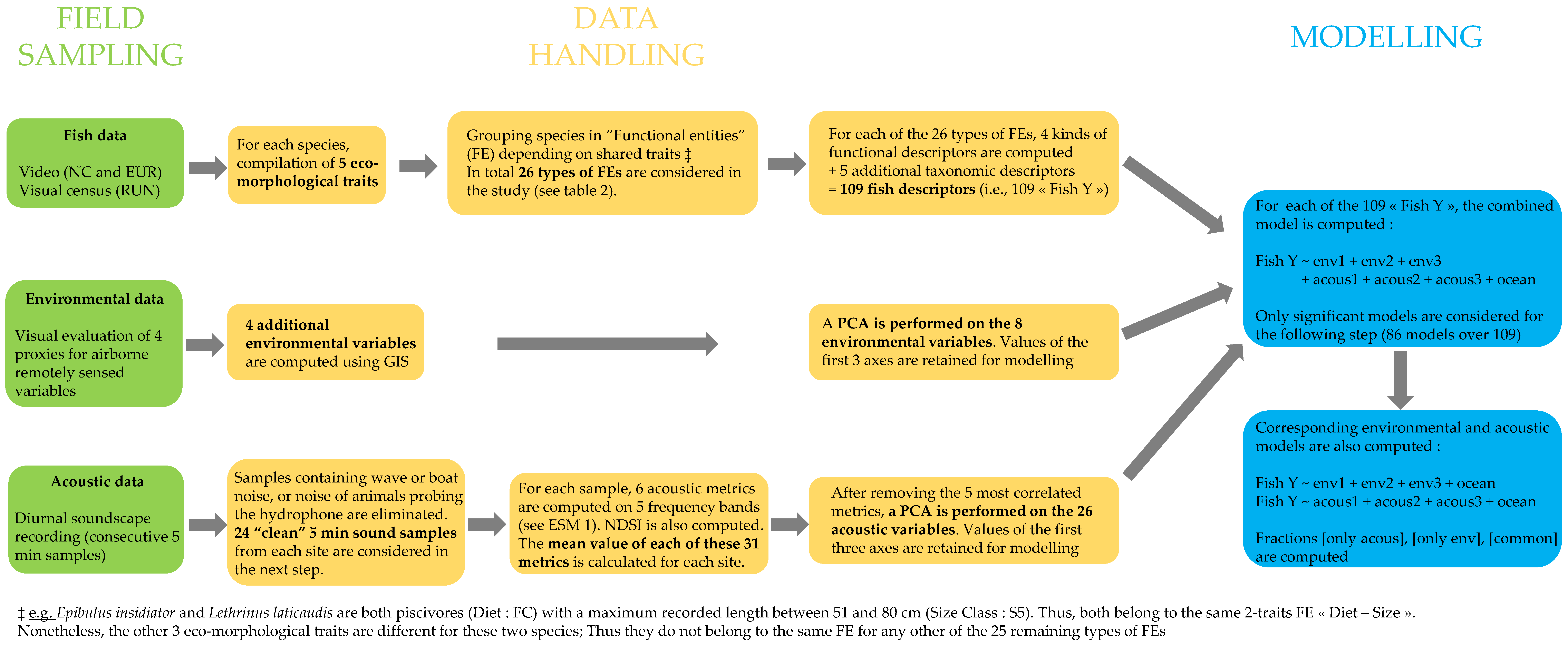
2. Materials and Methods
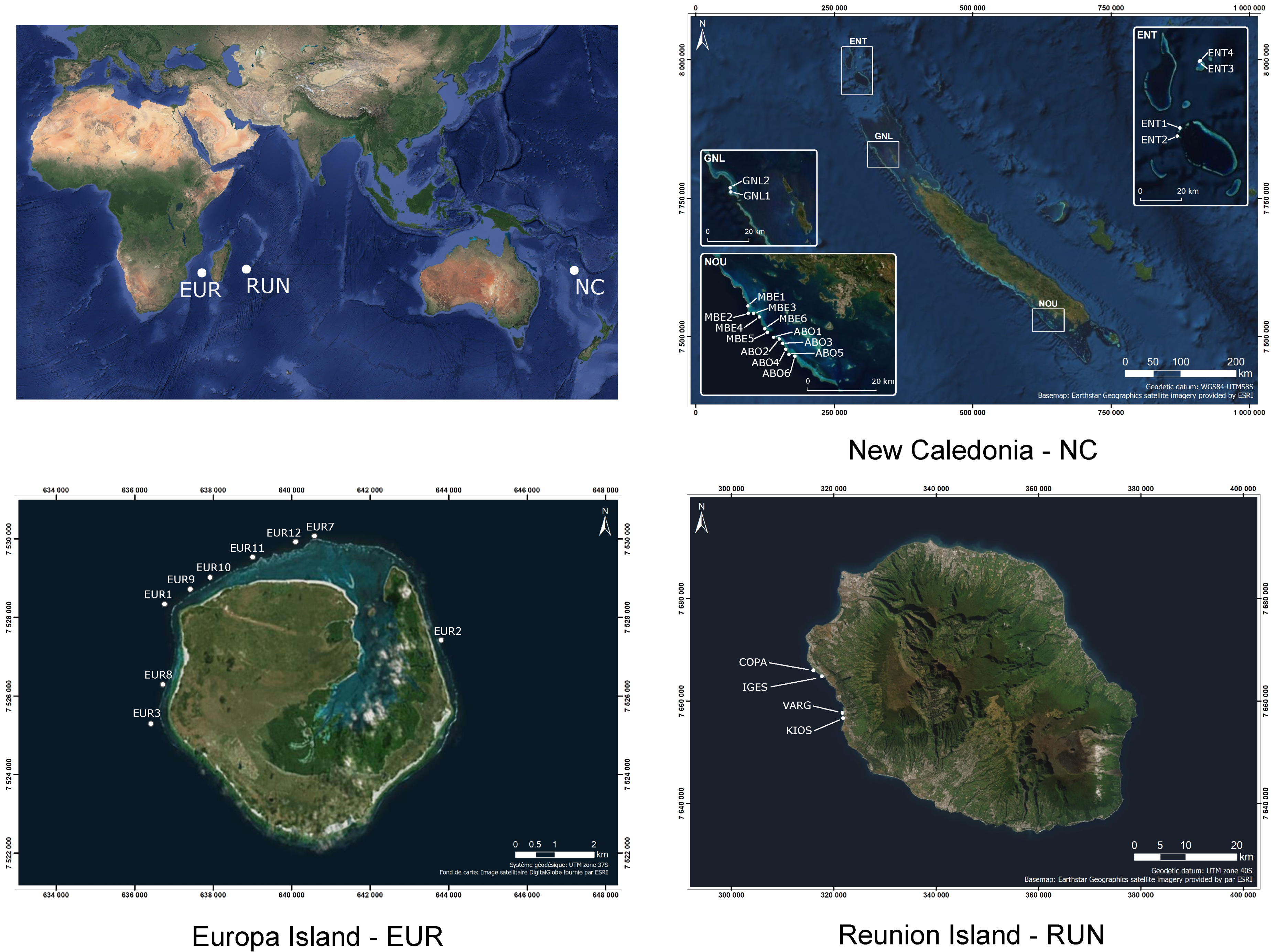
2.1. Study Sites

The study was conducted at 31 outer reef slope sites located between 10 and 18 m depth around three Indo-Pacific islands (Figure 1). Four sites were sampled in Reunion Island and nine sites in Europa Island, both located in the South-West Indian Ocean. The 18 other sites were sampled around New Caledonia in the South-West Pacific Ocean. Reunion Island reefs are exposed to strong anthropogenic pressures from a population of approximately 850,000 inhabitants and 500,000 visiting tourists annually, those of Europa Island are virtually pristine with strong protection implemented for decades and no people living within a 300 km radius around the island. New Caledonia is inhabited by approximately 270,000 inhabitants, of which 180,000 live in or near the capital Noumea. Twelve sites were located within a 30 km radius around Noumea, with six sites inside the Aboré Marine Protected Area and six sites outside. The remaining six sites were virtually pristine reefs (Great Northern Lagoon and d’Entrecasteaux reefs) located over 450 km away from Noumea. Reunion Island sites were sampled in October 2016, New Caledonia sites in July 2017, and Europa Island sites in April 2018.

2.2. Evaluation of Reef Fish Assemblage Characteristics

Video footage was used to evaluate reef fish assemblages at Europa Island and New Caledonia sites (e.g., [35]). Calibrated stereo-cameras (two GoPro cameras, San Mateo, CA, USA) affixed 50 cm above the substrate filmed for 90 min an area covering approximately 150 m2. Cameras were oriented so that footage captured half the substrate and half the water column above. We identified individual fish and estimated an index of abundance and biomass for each species using the software EventMeasure (SeaGIS, Bacchus Marsh, Australia). The maximum abundance “MaxN” for a species was calculated as the maximum number of individuals of this species that can be observed on a single frame of the footage. Size of these individuals was measured and their biomass evaluated to calculate the maximum biomass “MaxB” of the species. The coefficients “a” and “b” which define the relationship between fish length and weight for each species were extracted from FishBase [36].
Video footage was not performed at the four Reunion Island sites. At each of these sites, reef fish assemblages were visually evaluated using Underwater Visual Census (UVC; e.g., [37]) along three 5 × 30 m belt transects. During each census, a diver swam 1 m above the transect line identifying, counting, and evaluating the sizes (to the nearest cm) of all fishes within 2.5 m on either side of the central line. Highly mobile and wary species were enumerated on the first pass as the transect line was laid and all the remaining species during the second pass. Transects encompassed half of the water column. As for video footage, the vast majority of individuals were found within a few meters above the seafloor. All detected fishes were recorded.
To homogenise the results of visual censuses and video footage and thus combine visual and video data in the modelling step, visual observations were averaged among the three transects at each Reunion site (e.g., for a given site, abundance of species “s” was the mean abundance of this species among the three transects, etc.). Indeed, a single 30 m belt transect covers approximately a 150 m2 area, equivalent to the coverage of video footage.
For each species recorded in the study, eco-morphological traits were compiled from FishBase [36] according to the classification used in recent articles (e.g., [38]). Five traits were considered: diet, species size class, schooling, mobility, and level in the water column. Three to six levels were considered for each trait (Table 1).
Species sharing similar eco-morphological traits were grouped into “Functional entities” (annotated “FE”). Each FE was considered as a proxy for the ecological function performed by a group of species following an approach increasingly used over the past decade (see [39]).
We estimated five taxonomic descriptors of fish assemblages: species richness, total abundance, total biomass, and two Shannon indices, one calculated on species abundance and another on species biomass (i.e., taxonomic distribution of abundance and biomass).
Functional descriptors were based on functional entities (FEs) rather than species. Four kinds of descriptors were calculated: functional richness (i.e., number of FEs) and three Shannon indices calculated on the distribution of species richness, abundance, or biomass among FEs (henceforth called functional distribution of richness, abundance, and biomass respectively). We considered FEs of increasing levels of complexity (i.e., from two to five eco-morphological traits), with all possible combinations of traits for each level (Table 2). The simplest FEs combined two eco-morphological traits (e.g., diet-size or diet-schooling), resulting in 10 types of 2-trait FEs. Similarly, we considered ten types of 3-trait FEs, five types of 4-trait FEs, and one type of 5-trait FEs. In total 26 types of FEs were considered in the study. Thus, a total of 104 functional descriptors was computed (four kinds of descriptors * 26 types of FEs). Biomass was log-transformed prior to the calculation of biomass-related descriptors.

2.3. Environmental Variables

Eight environmental characteristics were considered at each site, comprising reef habitat features and human pressure. The eight variables were selected on the condition that they could be easily retrieved over large areas.
Four environmental variables were computed using open-source GIS layers available at world scale. Exposure to waves was determined as being between 1 (low) and 3 (high), based on site orientation and knowledge of dominant swells, using the layer of the global distribution of warm-water coral reefs [40]. The same layer was used to compute coral reef area within a 12 km radius around each site. Gravity (i.e., human disturbance based on population size surrounding a reef site and travel time to the nearest population centre) was evaluated using the layer of gravity estimates within 500 km [19]. These three variables were computed using QGIS [41]. Based on the World Database on Protected Area [42], three management statuses were considered: (1) Fished, (2) Marine Protected Area, and (3) Pristine Area.
The other four environmental variables represented coarse habitat features that could have been estimated using airborne remote sensing tools. Indeed, reef slope and habitat complexity can be evaluated using airborne LIDAR (e.g., [17]), live coral cover using airborne hyperspectral imagery (e.g., [10]), and soft bottom cover using satellite imagery (e.g., [9]). Unfortunately, such airborne remotely sensed data were not simultaneously available for the three localities in our study and datasets of habitat features available at world scale (e.g., Allen Coral Atlas) are only qualitative at this time (e.g., “coral/algae” benthic map class does not differentiate between 5 and 50% of coral cover). To approximate the precision that could have been obtained using airborne remote sensing tools, we visually estimated these four variables during a short dive at each of the 31 sites using semi-quantitative scales. At each site, we determined an area representative of the site habitat (~150 m2) and visually estimated the four habitat variables as follows. Habitat complexity ranged from 0 (flat landscapes) to 5 (exceptionally complex habitats with numerous caves and overhangs; see [43]) as illustrated in the Supplementary Materials of Darling et al. [22]. Live coral cover was divided into five semi-quantitative categories (see [44]): 1 (0–20%); 2 (20–30%); 3 (30–40%); 4 (40–50%), and 5 (>50%). Similarly, five semi-quantitative categories for soft bottom cover were defined: 1 (0–5%); 2 (5–10%); 3 (10–20%); 4 (20–30%), and 5 (>30%). Slope was evaluated as being between 1 (gentle) and 3 (steep).

2.4. Soundscape Recordings and Acoustic Metrics

At each site, soundscapes were continuously recorded between 9:30 am and 3:30 pm simultaneously with video footage recorded at Europa Island (April 2018) and New Caledonia (July 2017), and the day before the underwater visual census at Reunion Island (April 2016).
Two identical recording systems were alternatively used. Systems were affixed to the substrate to prevent movement during recordings. Each system was composed of a TC 4014–5 omnidirectional hydrophone (RESON, Slangerup, Denmark) fixed approximately 1.5 m above the substrate at the top of an aluminium tripod and connected to an acquisition chain designed by NORTEKMED S.A.S (Toulon, France). Sensitivity of the whole recording system was −166 dB re 1 V μPa−1. Calibration of the systems was regularly checked during the study with a Brüel & Kjaer 4229 hydrophone calibrator (Nærum, Denmark). Systems were programmed to record continuously at 100 kHz and 16 bits, providing an analysis range of 0–50 kHz.
Samples containing wave or boat noise, or noise of animals probing the hydrophone were eliminated in order to keep 24 “clean” 5 min sound samples from each site. This recording protocol was found to be well-suited to acoustically discriminate coral reef sites [45]. Although this snapshot approach fails to capture the vast spatio-temporal variabilities in reef soundscapes [31], here the aim was to test if it could provide information about the structure of the reef fish assemblage present at the moment of the recording.
For each sound sample, six acoustic metrics were calculated on five frequency bands (0.1–0.5 kHz; 0.5–1 kHz; 1–2 kHz; 2–7 kHz; 0.1–50 kHz): amplitude (Sound Pressure Level; SPL), Bioacoustics Index (BI), spectral entropy (sh), temporal entropy (th), acoustic entropy index (H), and Acoustic Complexity Index (ACI). In addition, the Normalised Difference Soundscape Index (NDSI) was calculated to evaluate the ratio of high-frequency (2–7 kHz) to low-frequency (0.1–1 kHz) acoustic components (see Supplementary Materials ESM 1 for details on acoustic metrics and their calculation). Both the acoustic metrics and frequency bands were selected following the results previously obtained on coral reefs (e.g., [14,33,34,45]).
After removing the most-correlated metrics [H (0.5–1 kHz), H (2–7 kHz), BI (2–7 kHz), sh (2–7 kHz), and th (2–7 kHz)], 26 acoustic metrics were retained for each sound sample. The mean value of each metric was computed for each site.

2.5. Statistical Analyses

2.5.1. Reduction of Environmental Data and Acoustic Data

To summarise the information provided by environmental and acoustic variables and avoid model over-fitting, we performed a Principal Component Analysis on both sets of explanatory variables prior to modelling and retained the first three axes of each (annotated env1, env2, env3 and acous1, acous2, acous3).

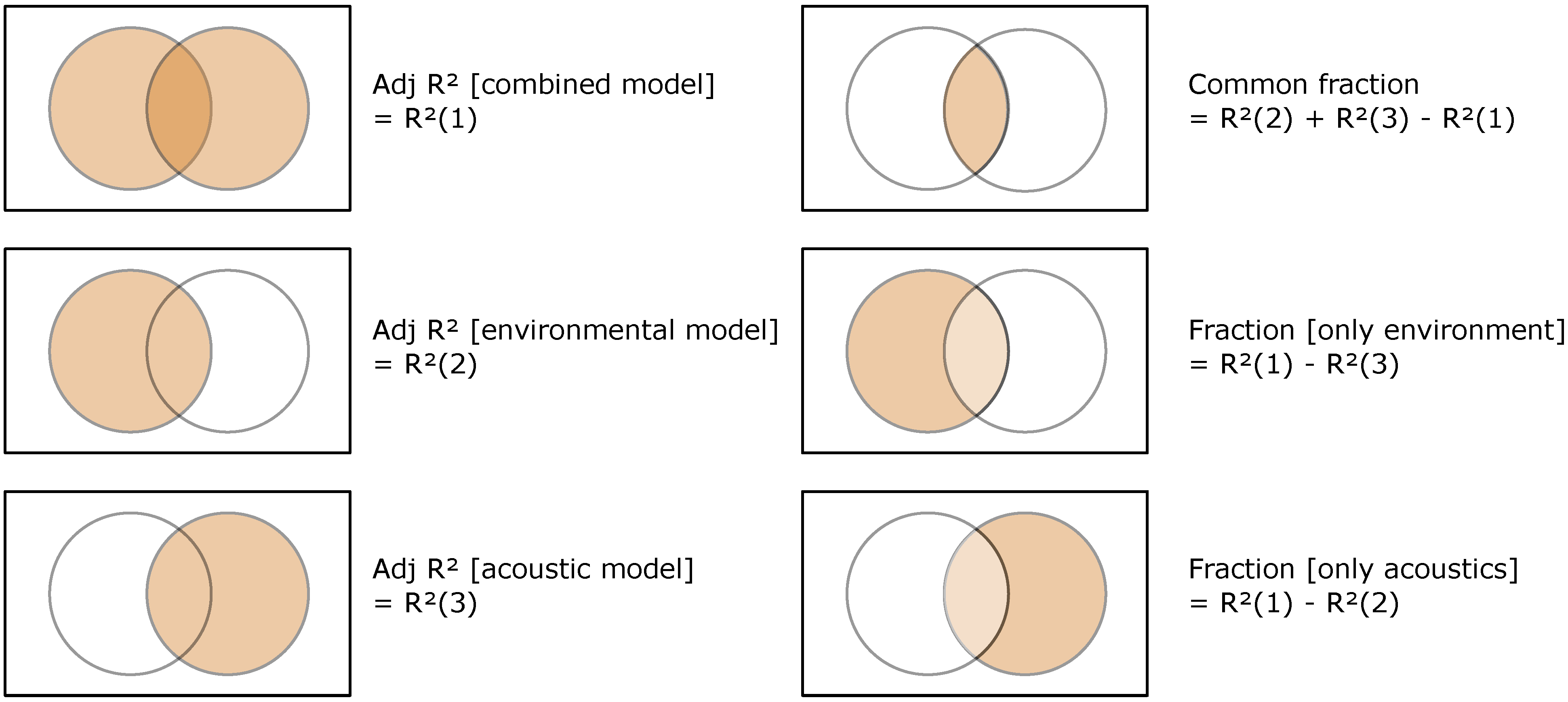
2.5.2. Test of the Added Value of Acoustic data in Predicting Fish Assemblage Characteristics

We first used linear models to evaluate the performance of combined environmental and acoustic data in predicting each of the 109 fish descriptors (104 functional descriptors and 5 taxonomic descriptors). When models were significant, we followed the same approach using environmental data and then using acoustic data. Hence, three linear models were built for each of the 109 fish descriptors, theoretically representing 327 models. Among these, 16 were expected to be statistically significant just by chance at an alpha level of 0.05, which must be considered in results interpretation. Models were built as follows:
(combined) Fish ~ env1 + env2 + env3 + acous1 + acous2 + acous3 + ocean
(environment) Fish ~ env1 + env2 + env3 + ocean
(acoustics) Fish ~ acous1 + acous2 + acous3 + ocean
When ocean effect was not significant in the combined model, it was removed from the analyses.
Adjusted coefficients of determination (i.e., adjusted R2) were examined for the three models. We used variation partitioning ([46]; Figure 2) to quantify the unique fractions of variation in each of the 109 fish descriptors explained by environmental variables, by acoustic variables (i.e., the added value of using acoustic variables), as well as the fraction explained by both (i.e., common fraction).

2.5.3. Identification of the Fish Assemblage Characteristics Best Predicted by Acoustic Data

To better understand the information provided by acoustic variables, we used linear models to examine how the adjusted R2 of acoustic models (or the fraction only explained by acoustic variables) was influenced by the number of traits considered in the FE and by the identity (e.g., diet, size class) of those traits. For each kind of functional descriptor (i.e., functional richness, functional distribution of richness, etc.), the effect of considering a particular trait (diet, species size class, schooling, mobility, and level in the water column) in the FEs was tested. This represented 20 tests on adjusted R2 of the acoustic models and 20 tests on fractions [only acoustics].
The whole methodological approach that was followed from sampling to data analysis is synthetised in Figure 3. All datasets are available in Supplementary Materials (ESM 2 to 8).

3. Results

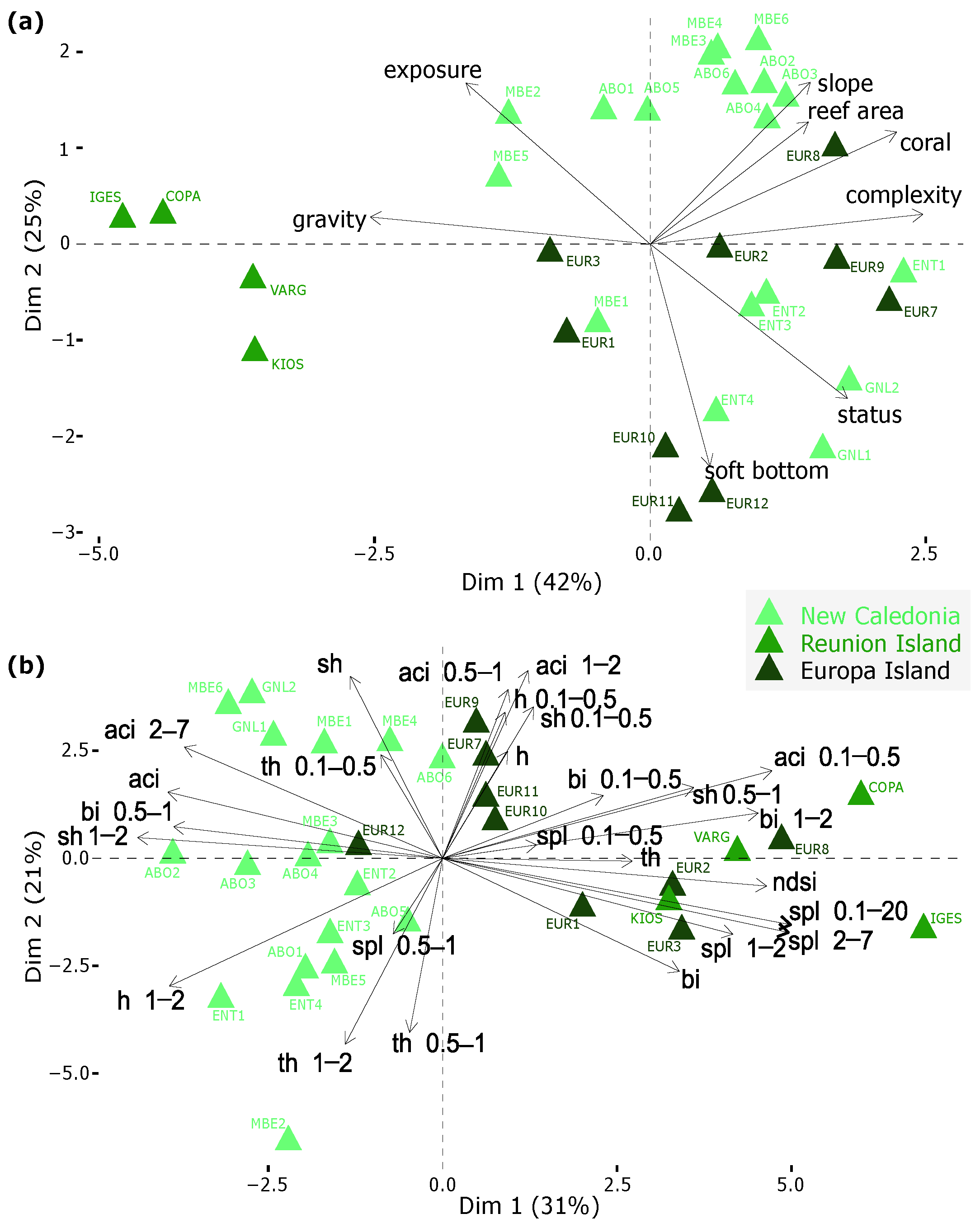
3.1. Reduction of Environmental Data and Acoustic Data

The first three axes of the Principal Component Analysis performed on the environmental variables explained 79% of the variance among the sites. For the Principal Component Analysis performed on the acoustic variables, the first three axes explained 70% of the variance (Figure 4).

3.2. Test of the Added Value of Acoustic Data in Predicting Fish Assemblage Characteristics

Of the 109 combined models, 86 were significant. Depending on the fish descriptor considered, the adjusted R2 ranged from 0.14 to 0.60 for the environmental models [mean value (±sd) = 0.35 ± 0.09], from 0 to 0.47 for the acoustic models [mean value (±sd) = 0.14 ± 0.15], and from 0.21 to 0.58 for the combined models [mean value (±sd) = 0.39 ± 0.09] (Figure 5a,c).
The contribution of the acoustic variables to the variance explained by the combined models, i.e., fraction [only acoustics], varied greatly. It ranged from −0.05 to 0.22 [mean value (±sd) = 0.04 ± 0.05] (Figure 5a). This contribution was positive for 69% of the fish descriptors tested (59 descriptors over 86) and negative for the remaining 31%, revealing that the acoustic data did not bring additional explicative power to the environmental models for these 27 descriptors (Figure 5a). These latter descriptors reflected the total abundance, the taxonomic distribution of biomass, and several descriptors of the functional richness, functional distribution of richness, and functional distribution of biomass.
The explicative power of the combined models significantly increased with the fraction of variation only explained by acoustics (Pearson’ρ = 0.27, p < 0.05) (i.e., when fraction [acoustics] was high, adjusted R2 of the combined model was also high, Figure 5a), revealing that, overall, the acoustic data significantly enhanced the explicative power of the environmental models.
We found no significant relationship between the fraction only explained by the acoustic variables and the fraction only explained by the environmental variables (Pearson’ρ = −0.19, p = 0.08) (Figure 5b), or between the fraction only explained by the acoustic variables and the common fraction (Pearson’ρ = 0, p = 0.94). This absence of significant relationships shows that the information only provided by the acoustic data, albeit limited (i.e., maximum value = 0.22), is independent of the information provided by the environmental data. In other words, a low fraction (either acoustic or environmental) does not imply that the other fraction is low, which highlights the complementarity between both datasets in explaining the structures of reef fish assemblages. Nonetheless, the fraction only explained by the environmental variables was greater than the fraction only explained by the acoustic variables in a majority of cases (i.e., most of the points are below the y = x line; Figure 5b).
The fractions only explained by the environmental variables reached the highest values for a number of descriptors of functional richness and functional distribution of biomass (Figure 5a,c). For other descriptors, particularly those reflecting the functional distribution of abundance, the fraction only explained by the environmental variables was lower than the fraction only explained by the acoustic variables (Figure 5b). As such, with this larger contribution of acoustic variables where environmental variables performed poorly (Figure 5c), the combined models were found to predict a wide range of descriptors of the fish assemblage structure. The Ocean basin was significant in 34% of combined models including all the models of the functional distribution of abundances.
To sum up, the acoustic data globally enhanced the predictions of fish assemblage characteristics with respect to the predictions only based on the environmental data. Albeit limited (i.e., mean value = 0.04 and maximum value = 0.22), the contribution of the acoustic data was positive for 69% of the fish descriptors tested and was globally not correlated to the contribution of the environmental data, which highlights that the information provided by both data types is different. In addition, the contribution of the acoustic data was higher than the contribution of the environmental data for predicting the functional distribution of fish abundance.

3.3. Identification of the Fish Assemblage Characteristics Best Predicted by the Acoustic Data

Concerning functional descriptors, the adjusted R2 for the acoustic models were significantly affected by the type of functional descriptor (ANOVA, F = 26.22, df = 3, p < 10−10) and by the number of traits considered to construct the FEs (ANOVA, F = 21.79, df = 1, p < 10−4); these effects were independent (interaction term, F = 1.29, df = 3, p = 0.28) (Table 3).
The adjusted R2 of the acoustic models was significantly higher for the functional distributions of abundance than for the other functional descriptors (all p < 10−6, Table 4 and Figure 6) and significantly decreased with increasing functional resolution (i.e., an increasing number of traits considered to construct the FEs) (slope = −0.06, t = −4.641, p < 10−4).
The number and identity of traits influenced the models. When the level in the water column was considered in the 2-trait FEs, the adjusted R2 of the acoustic models was significantly higher than when this trait was not considered for functional richness and for the functional distributions of biomass (Figure 7a,b). Nonetheless, this trait was not significantly influential when considering the fraction only explained by the acoustics. This suggests that the predictions by the acoustic and environmental data were partially redundant when the FEs included the level in the water column.
When diet was considered in the FE composition, the fraction only explained by the acoustic variables was significantly enhanced for the functional distribution of biomass (Figure 7c), revealing the particular added value of the acoustic variables in predicting diet-related biomass. On the contrary, considering size class and schooling in the FE composition significantly dropped the adjusted R2 of the acoustic models for the functional distribution of richness and abundance, respectively (Figure 7d,e).

4. Discussion

Tropical coral reefs are extremely different from one region to another, but they also notably vary at local scales (e.g., [47]). Adding that the intensity of human disturbances strongly differs between localities, the response of coral reef ecosystems to ongoing changes is highly spatialized and hard to predict and may rapidly change in a given locality [2,3,4,48]. Therefore, long-term adaptive management needs efficient monitoring networks able to track changes both within and across regions identified as conservation priorities [3]. Since this fundamentally requires frequent and standardised information across scales, the capacity of observer-based in situ monitoring to respond to this challenge may be limited [7]. Concurrently, remote sensing is considerably augmenting our monitoring capacities with the recent emergence and diversification of affordable tools [7,49,50] combined with the increasing possibilities of automated handling through machine learning (e.g., [51,52,53,54]). Although remote sensing offers opportunities to solve numerous monitoring challenges (i.e., standardised information from a local to a global scale, frequent assessments), its optimisation for conservation requires addressing several barriers [7,31,50]. Among these, the ecological significance of remotely sensed data still needs to be specified, as well as the capacity of these data to reliably inform EOVs [7,50]. Also, the complementarity among remote sensing tools must be understood in order to optimise their simultaneous implementation (e.g., [17,55,56,57]).
Consistent with the results of previous studies (e.g., [17,19,23]), we found that coarse environmental data (i.e., variables that could have been estimated using airborne remote sensing tools and variables extracted from GIS layers) could provide sufficient information to delineate multiple aspects of the structure of reef fish assemblages across the Indo-Pacific region. The novelty of our study was to demonstrate that PAM data could improve these predictions. Indeed, the acoustic data significantly enhanced the explicative power of the environmental models. Also, the acoustic variables performed better than the environmental variables for predicting the functional distribution of fish abundance. Although the magnitude of improvements was low, our results revealed that the acoustics metrics could supply different, and thus complementary, information to the airborne remotely sensed data.
This was not the case, however, for the prediction of the taxonomic descriptors. This contrasts with previous findings on coral reefs where several acoustic metrics were correlated with fish species’ richness and abundance (i.e., SPL and ACI in the lower frequencies; e.g., [14,32,33]). Two elements may explain this discrepancy. First, in this study we considered the synthetic information from a panel of 26 acoustic metrics (i.e., values of the first three axes of a PCA on these metrics) rather than the individual metrics examined in previous studies. Second, the taxonomic structures of fish assemblages were strongly different among our study sites as they were located in different biogeographic contexts. This may have interfered with the capacity of the acoustic metrics to reflect the taxonomic descriptors between distant localities. The lack of performance of PAM for predicting the taxonomic descriptors at this scale illustrates that other remote sensing tools, such as eDNA metabarcoding surveys (e.g., [15]), could better complement airborne tools for taxonomic assessments.
Although the predictions of functional descriptors were also affected by biogeographic effects (significant in 34% of the models), PAM alone explained the different levels of variation in the distribution of richness, abundance, and biomass across the FEs and in the functional richness of coral reef fish assemblages. The contribution of PAM was particularly important for predicting the functional distribution of abundance, as environmental variables were less performant regarding this aspect. These results illustrate that simultaneously using several remote sensing tools could generate more comprehensive evaluations of coral reef fish assemblages.
Furthermore, our approach allowed for the identification of the functional aspects for which the prediction by PAM offered a significant added value. The best predictions were obtained for coarse functional classifications (i.e., 2-trait FEs), whereas increasing the functional resolution resulted in poorer descriptions. These results suggest that the distribution of ecological functions among fish species, when considered at a relatively coarse level, is reflected in the soundscape composition. Different fish species ensuring a similar ecological function may produce similar acoustic patterns through feeding, movements, and defense, for example. This is consistent with the results of a previous study where the abundance and biomass of several simple fish FEs were found to significantly correlate with various acoustic metrics [34].
In addition, the PAM predictions were significantly enhanced when considering diet and the level in the water column in the FE composition. Numerous acoustic signals are linked with feeding, such as predation, escape, and parrotfish scraping (see review by Lobel et al. [58]), partially explaining why this trait emerged from the analysis. Furthermore, the level in the water column occupied by a species is linked to its detectability by the hydrophone (i.e., hydrophone range to the fish), which could explain at least partially why this trait also emerged. Moreover, this could be related to differences in the prevalence of soniferous fish among demersal, semi-demersal, and pelagic categories.
Surprisingly, considering size class (and to a lesser extent schooling) reduced the predictive capacity of PAM, whereas these traits are usually important features structuring sound production by fishes (e.g., [59]). Beyond the question of which functional information is conveyed through soundscapes, these results suggest that considering local specificities is crucial when defining the functional role of individuals. Indeed, there were important differences between the theoretical and the actual observed size class/schooling classifications of species depending on the study sites (e.g., for some species in Reunion Island, the observed maximum size was much lower than the theoretical maximum size). This could explain the poorer results when considering these traits across sites.
A limit of the study was the discrepancy between fish survey methods, which may have introduced some biases, especially in the evaluation of cryptic species. Although numerous studies have evaluated the implications of using different survey methods (e.g., UVC, Baited Remote Underwater stereo-Videos, Diver Operated stereo-Videos, Rotating Videos) on the assessment of coral reef fish assemblages (e.g., [60,61,62,63]), we did not find any study considering a video protocol similar to that used in the present study (i.e., 90 min video footage using UnBaited Remote Underwater stereo-Videos, UBRUV). However, in their study of tropical seagrass meadows, Zarco-Perello and Enríquez [64] found that UVC provided lower estimations of fish diversity and abundance when compared to UBRUV, especially for herbivorous and piscivorous fishes [64]. Since we used similar UVC and UBRUV protocols, our evaluation of the fish assemblage structure could have been biased at Reunion Island.
PAM is an emerging approach for ecosystem monitoring, which will rapidly gain in performance with upcoming developments. For example, in this study, we made a subjective selection of acoustic variables to discriminate among soundscapes, whereas the development of data-driven approaches (e.g., convolutional neural networks) allows for a more exhaustive and objective selection of the acoustic features able to discriminate among soundscapes (see e.g., [54]). Also, most studies, including the present one, still refer to a known referential (here the visual assessment of fish assemblages) to evaluate PAM capacities. Alternative approaches (e.g., automated classification and quantification of biological signals using machine learning algorithms) will probably bring out the best in the PAM applications. Although deployments of acoustic devices only last a few minutes, they still require in situ human presence. We may expect that Automated Underwater (or Surface) Vehicles will be able to replace humans in this task in a few years. By integrating onboard data handling, analysis, and transmission, they could considerably improve coral reef PAM over ever larger areas.

5. Conclusions

This study represents the first test of the complementarity between coarse environmental data (including data which could have been collected using airborne remote sensing tools) and PAM for coral reef fish assemblage assessment. Although our results highlight a relatively low added value of combining PAM with environmental data, they should be considered as an incentive to develop more robust studies. The latter could at least include more sites and rely on a single standardised method (e.g., video footage) for establishing a “reference” assessment for fish assemblages. They could also widely benefit from integrating the perspectives cited above.
Despite its weaknesses, our study showed that acoustic data could be more relevant than environmental data for predicting certain aspects of the fish assemblages (i.e., functional distribution of abundance). In addition, the significant improvements obtained when considering diet and the level in the water column in the FE composition strongly suggest the potential of PAM for assessing various aspects of fish assemblage functional structure. Moreover, as acoustic data were collected over a few hours, our results highlight that PAM can deliver useful in situ snapshot information.

Supplementary Materials

The following supporting information can be downloaded at: https://www.mdpi.com/article/10.3390/rs14102394/s1. ESM1: calculation of acoustic metrics: ESM2: values of acoustic metrics on each site; ESM3: values of environmental variables on each site; ESM4: values of fish taxonomic variables on each site; ESM5: value of fish functional richness on each site; ESM6: value of functional distribution of fish species richness on each site; ESM7: value of functional distribution of fish abundance on each site; ESM8: value of functional distribution of fish biomass on each site. References [65,66,67,68,69,70,71,72,73,74] are cited in the Supplementary Material ESM1.

Author Contributions

Conceptualization, S.E., F.G., M.K. and J.H.B.; Data curation, S.E., F.G., G.M.-T., I.U.-B. and L.V.; Formal analysis, S.E. and F.G.; Funding acquisition, S.E., I.U.-B., L.V. and J.H.B.; Investigation, S.E., I.U.-B., L.V. and J.H.B.; Methodology, S.E., F.G., L.V., M.K. and J.H.B.; Project administration, S.E. and J.H.B.; Resources, S.E., I.U.-B., L.V. and J.H.B.; Software, F.G.; Supervision, J.H.B.; Validation, F.G.; Visualization, S.E.; Writing–original draft, S.E.; Writing–review and editing, F.G., G.M.-T., I.U.-B., L.V., M.K. and J.H.B. All authors have read and agreed to the published version of the manuscript.

Funding

S.E. and I.U.-B. were supported by a CIFRE fellowship (French ANRT; agreement numbers 2015/1538 and 2017/0322). Part of this study was funded by the European Commission (DG DEVCO) through the BEST 2.0 program (CORCOPA project).

Data Availability Statement

All datasets are available as Supplementary Material. Research was authorized by the RNMR (Reunion Island), the TAAF (Europa Island), and the Government of New Caledonia (Apex program).

Acknowledgments

We are grateful to Valentin Bouvot, Sophie Bureau, Lucas Bonnin, Germain Boussarie, Bertrand Bourgeois, Armand Dayde, Eric Folcher, Erwan Meyer, and Franco Nirvola for field assistance. We thank the crews of the yacht Antsiva and the research vessel Amborella, the pilots of the Archamia and Mangabe, the military forces (FAZSOI), and Ocean Innovation Tour for logistical support. We thank Jessica Meeuwig for use of the EventMeasure software.

Conflicts of Interest

We declare we have no competing interest.

References

  1. Harborne, A.; Rogers, A.; Bozec, Y.; Mumby, P.J. Multiple Stressors and the Functioning of Coral Reefs. Annu. Rev. Mar. Sci. 2016, 9, 445–468. [Google Scholar] [CrossRef] [PubMed]
  2. Hughes, T.P.; Barnes, M.L.; Bellwood, D.R.; Cinner, J.E.; Cumming, G.S.; Jackson, J.B.; Kleypas, J.; Van De Leemput, I.A.; Lough, J.M.; Morrison, T.H.; et al. Coral reefs in the Anthropocene. Nature 2017, 546, 82–90. [Google Scholar] [CrossRef] [PubMed]
  3. Hoegh-Guldberg, O.; Kennedy, E.V.; Beyer, H.L.; McClennen, C.; Possingham, H.P. Securing a long-term future for coral reefs. Trends Ecol. Evol. 2018, 12, 936–944. [Google Scholar] [CrossRef] [PubMed] [Green Version]
  4. Williams, G.J.; Graham, N.A.J. Rethinking coral reef functional futures. Funct. Ecol. 2019, 33, 942–947. [Google Scholar] [CrossRef]
  5. Bellwood, D.R.; Pratchett, M.S.; Morrison, T.H.; Gurney, G.G.; Hughes, T.P.; Álvarez-Romero, J.G.; Day, J.C.; Grantham, R.; Grech, A.; Hoey, A.S.; et al. Coral reef conservation in the Anthropocene: Confronting spatial mismatches and prioritizing functions. Biol. Conserv. 2019, 236, 604–615. [Google Scholar] [CrossRef]
  6. Duarte, C.M.; Agusti, S.; Barbier, E.; Britten, G.L.; Castilla, J.C.; Gattuso, J.P.; Fulweiler, R.W.; Hughes, T.P.; Knowlton, N.; Lovelock, C.E.; et al. Rebuilding marine life. Nature 2020, 580, 39–51. [Google Scholar] [CrossRef]
  7. Obura, D.O.; Aeby, G.; Amornthammarong, N.; Appeltans, W.; Bax, N.J.; Bishop, J.; Brainard, R.E.; Chan, S.; Fletcher, P.; Gordon, T.A.; et al. Coral reef monitoring, reef assessment technologies, and ecosystem-based management. Front. Mar. Sci. 2019, 6, 580. [Google Scholar] [CrossRef] [Green Version]
  8. Roelfsema, C.M.; Kovacs, E.; Ortiz, J.C.; Wolff, N.H.; Callaghan, D.; Wettle, M.; Ronan, M.; Hamylton, S.M.; Mumby, P.J.; Phinn, S. Coral reef habitat mapping: A combination of object-based image analysis and ecological modelling. Remote Sens. Environ. 2018, 208, 27–41. [Google Scholar] [CrossRef]
  9. Roelfsema, C.M.; Kovacs, E.M.; Ortiz, J.C.; Callaghan, D.P.; Hock, K.; Mongin, M.; Johansen, K.; Mumby, P.J.; Wettle, M.; Ronan, M.; et al. Habitat maps to enhance monitoring and management of the Great Barrier Reef. Coral Reefs 2020, 39, 1039–1054. [Google Scholar] [CrossRef]
  10. Bajjouk, T.; Mouquet, P.; Ropert, M.; Quod, J.P.; Hoarau, L.; Bigot, L.; Le Dantec, N.; Delacourt, C.; Populus, J. Detection of changes in shallow coral reefs status: Towards a spatial approach using hyperspectral and multispectral data. Ecol. Indic. 2019, 96, 174–191. [Google Scholar] [CrossRef]
  11. González-Barrios, F.J.; Álvarez-Filip, L. A framework for measuring coral species-specific contribution to reef functioning in the Caribbean. Ecol. Indic. 2018, 95, 877–886. [Google Scholar] [CrossRef]
  12. Obura, D.O.; Gudka, M.; Rabi, F.A.; Gian, S.B.; Bijoux, J.; Freed, S.; Maharavo, J.; Mwaura, J.; Porter, S.; Sola, E.; et al. Coral Reef Status Report for the Western Indian Ocean (2017). In Nairobi Convention; Global Coral Reef Monitoring Network (GCRMN)/International Coral Reef Initiative (ICRI); Indian Ocean Commission: Port Louis, Mauritius, 2017. [Google Scholar]
  13. Mellin, C.; Parrott, L.; Andréfouët, S.; Bradshaw, C.J.A.; MacNeil, M.A.; Caley, M.J. Multi-scale marine biodiversity patterns inferred efficiently from habitat image processing. Ecol. Appl. 2012, 22, 792–803. [Google Scholar] [CrossRef] [PubMed] [Green Version]
  14. Staaterman, E.; Ogburn, M.B.; Altieri, A.H.; Brandl, S.J.; Seemann, J.; Whippo, R.; Goodison, M.; Duffy, J.E. Bioacoustic measurements complement visual biodiversity surveys: Preliminary evidence from four shallow marine habitats. Mar. Ecol. Prog. Ser. 2017, 575, 207–215. [Google Scholar] [CrossRef] [Green Version]
  15. West, K.M.; Stat, M.; Harvey, E.S.; Skepper, C.L.; DiBattista, J.D.; Richards, Z.T.; Travers, M.J.; Newman, S.J.; Bunce, M. eDNA metabarcoding survey reveals fine-scale coral reef community variation across a remote, tropical island ecosystem. Mol. Ecol. 2020, 29, 1069–1086. [Google Scholar] [CrossRef] [PubMed]
  16. Ouellette, W.; Getinet, W. Remote sensing for marine spatial planning and integrated coastal areas management: Achievements, challenges, opportunities and future prospects. Remote Sens. Appl. Soc. Environ. 2016, 4, 138–157. [Google Scholar] [CrossRef]
  17. Wedding, L.M.; Jorgensen, S.; Lepczyk, C.A.; Friedlander, A.M. Remote sensing of three-dimensional coral reef structure enhances predictive modeling of fish assemblages. Remote Sens. Ecol. Conserv. 2019, 5, 150–159. [Google Scholar] [CrossRef] [Green Version]
  18. Rappaport, D.I.; Royle, J.A.; Morton, D.C. Acoustic space occupancy: Combining ecoacoustics and lidar to model biodiversity variation and detection bias across heterogeneous landscapes. Ecol. Indic. 2020, 113, 106172. [Google Scholar] [CrossRef]
  19. Cinner, J.E.; Maire, E.; Huchery, C.; MacNeil, M.A.; Graham, N.A.J.; Mora, C.; McClanahan, T.R.; Barnes, M.L.; Kittinger, J.N.; Hicks, C.C.; et al. Gravity of human impacts mediates coral reef conservation gains. Proc. Natl. Acad. Sci. USA 2018, 115, E6116–E6125. [Google Scholar] [CrossRef] [Green Version]
  20. Purkis, S.J.; Gleason, A.C.R.; Purkis, C.R.; Dempsey, A.C.; Renaud, P.G.; Faisal, M.; Saul, S.; Kerr, J.M. High-resolution habitat and bathymetry maps for 65,000 sq. km of Earth’s remotest coral reefs. Coral Reefs 2019, 38, 467–488. [Google Scholar] [CrossRef] [Green Version]
  21. Friedlander, A.M.; Brown, E.K.; Jokiel, P.L.; Smith, W.R.; Rodgers, K.S. Effects of habitat, wave exposure, and marine protected area status on coral reef fish assemblages in the Hawaiian archipelago. Coral Reefs 2003, 22, 291–305. [Google Scholar] [CrossRef]
  22. Darling, E.S.; Graham, N.A.J.; Januchowski-Hartley, F.A.; Nash, K.L.; Pratchett, M.S.; Wilson, S.K. Relationships between structural complexity, coral traits, and reef fish assemblages. Coral Reefs 2017, 36, 561–575. [Google Scholar] [CrossRef] [Green Version]
  23. Barneche, D.R.; Rezende, E.L.; Parravicini, V.; Maire, E.; Edgar, G.J.; Stuart-Smith, R.D.; Arias-González, J.E.; Ferreira, C.E.; Friedlander, A.M.; Green, A.L.; et al. Body size, reef area and temperature predict global reef-fish species richness across spatial scales. Glob. Ecol. Biogeogr. 2019, 28, 315–327. [Google Scholar] [CrossRef]
  24. Moberg, F.; Folke, C. Ecological goods and services of coral reef ecosystems. Ecol. Econ. 1999, 29, 215–233. [Google Scholar] [CrossRef]
  25. Barbier, E.B.; Hacker, S.D.; Kennedy, C.; Koch, E.W.; Stier, A.C.; Silliman, B.R. The value of estuarine and coastal ecosystem services. Ecol. Monogr. 2011, 81, 169–193. [Google Scholar] [CrossRef]
  26. Rogers, A.; Blanchard, J.L.; Mumby, P.J. Fisheries productivity under progressive coral reef degradation. J. Appl. Ecol. 2018, 55, 1041–1049. [Google Scholar] [CrossRef]
  27. Pieretti, N.; Martire, M.L.; Farina, A.; Danovaro, R. Marine soundscape as an additional biodiversity monitoring tool: A case study from the Adriatic Sea (Mediterranean Sea). Ecol. Indic. 2017, 83, 13–20. [Google Scholar] [CrossRef]
  28. Carrasco, S.A.; Bravo, M.; Avilés, E.; Ruíz, P.; Yori, A.; Hinojosa, I.A. Exploring overlooked components of remote South-east Pacific oceanic islands: Larval and macrobenthic assemblages in reef habitats with distinct underwater soundscapes. Aquat. Conserv. Mar. Freshw. Ecosyst. 2021, 31, 273–289. [Google Scholar] [CrossRef]
  29. Ferrier-Pagès, C.; Leal, M.C.; Calado, R.; Schmid, D.W.; Bertucci, F.; Lecchini, D.; Allemand, D. Noise pollution on coral reefs?—A yet underestimated threat to coral reef communities. Mar. Pollut. Bull. 2021, 165, 112129. [Google Scholar] [CrossRef]
  30. Parsons, M.; Lin, T.H.; Mooney, A.; Erbe, C.; Juanes, F.; Lammers, M.; Li, S.; Linke, S.; Looby, A.; Nedelec, S.L.; et al. Sounding the Call for a Global Library of Underwater Biological Sounds. Front. Ecol. Evol. 2022, 10, 810156. [Google Scholar] [CrossRef]
  31. Mooney, T.A.; Di Iorio, L.; Lammers, M.; Lin, T.H.; Nedelec, S.L.; Parsons, M.; Radford, C.; Urban, E.; Stanley, J. Listening forward: Approaching marine biodiversity assessments using acoustic methods. R. Soc. Open Sci. 2020, 7, 201287. [Google Scholar] [CrossRef]
  32. Kennedy, E.V.; Holderied, M.W.; Mair, J.M.; Guzman, H.M.; Simpson, S.D. Spatial patterns in reef-generated noise relate to habitats and communities: Evidence from a Panamanian case study. J. Exp. Mar. Bio. Ecol. 2010, 395, 85–92. [Google Scholar] [CrossRef]
  33. Bertucci, F.; Parmentier, E.; Lecellier, G.; Hawkins, A.D.; Lecchini, D. Acoustic indices provide information on the status of coral reefs: An example from Moorea Island in the South Pacific. Sci. Rep. 2016, 6, 33326. [Google Scholar] [CrossRef] [PubMed] [Green Version]
  34. Elise, S.; Urbina-Barreto, I.; Pinel, R.; Mahamadaly, V.; Bureau, S.; Penin, L.; Adjeroud, M.; Kulbicki, M.; Bruggemann, J.H. Assessing key ecosystem functions through soundscapes: A new perspective from coral reefs. Ecol. Indic. 2019, 107, 105623. [Google Scholar] [CrossRef]
  35. Myers, E.; Harvey, E.; Saunders, B.; Travers, M. Fine-scale patterns in the day, night and crepuscular composition of a temperate reef fish assemblage. Mar. Ecol. 2016, 37, 668–678. [Google Scholar] [CrossRef]
  36. FishBase. 2019. Available online: http://www.fishbase.org/ (accessed on 20 December 2019).
  37. Labrosse, P.; Kulbicki, M.; Ferraris, J. Underwater Visual Fish Census Surveys; Secretariat of the Pacific Community: Nouméa, Nouvelle-Calédonie, 2002; 60p. [Google Scholar]
  38. Mellin, C.; Mouillot, D.; Kulbicki, M.; McClanahan, T.R.; Vigliola, L.; Bradshaw, C.J.A.; Brainard, R.E.; Chabanet, P.; Edgar, G.J.; Fordham, D.A.; et al. Humans and seasonal climate variability threaten large bodied coral reef fish with small ranges. Nat. Commun. 2016, 7, 10491. [Google Scholar] [CrossRef] [PubMed]
  39. Bellwood, D.R.; Streit, R.P.; Brandl, S.J.; Tebbett, S.B. The meaning of the term “function” in ecology: A coral reef perspective. Funct. Ecol. 2019, 33, 948–961. [Google Scholar] [CrossRef] [Green Version]
  40. UNEP-WCMC; WorldFish Centre; WRI; TNC. Global Distribution of Warm-Water Coral Reefs, Compiled from Multiple Sources Including the Millennium Coral Reef Mapping Project; Version 1.3; Includes Contributions from IMaRS-USF and IRD (2005), IMaRS-USF (2005) and Spalding et al. (2001); UNEP World Conservation Monitoring Centre: Cambridge, UK, 2010; Available online: http://data.unep-wcmc.org/datasets/1 (accessed on 15 January 2020).
  41. QGIS Development Team. QGIS Geographic Information System. Open Source Geospatial Foundation Project. 2018. Available online: http://qgis.osgeo.org (accessed on 15 January 2020).
  42. WDPA. 2020. Available online: https://www.protectedplanet.net/en (accessed on 15 January 2020).
  43. Polunin, N.V.C.; Roberts, C.M. Greater biomass and value of target coral-reef fishes in two small Caribbean marine reserves. Mar. Ecol. Prog. Ser. 1993, 100, 167. [Google Scholar] [CrossRef]
  44. English, S.; Wilkinson, C.; Baker, V. Survey Manual for Tropical Marine Resources, 2nd ed.; AIMS: Townsville, Australia, 1997. [Google Scholar]
  45. Elise, S.; Bailly, A.; Urbina-Barreto, I.; Mou-Tham, G.; Chiroleu, F.; Vigliola, L.; Robbins, W.D.; Bruggemann, J.H. An optimised passive acoustic sampling scheme to discriminate among coral reefs’ ecological states. Ecol. Indic. 2019, 107, 105627. [Google Scholar] [CrossRef]
  46. Legendre, P. Studying Beta Diversity: Ecological Variation Partitioning by Multiple Regression and Canonical Analysis. Chin. J. Plant Ecol. 2007, 31, 976–981. [Google Scholar] [CrossRef] [Green Version]
  47. Heenan, A.; Williams, G.J.; Williams, I.D. Natural variation in coral reef trophic structure across environmental gradients. Front. Ecol. Environ. 2020, 18, 69–75. [Google Scholar] [CrossRef]
  48. Beyer, H.L.; Kennedy, E.V.; Beger, M.; Chen, C.A.; Cinner, J.E.; Darling, E.S.; Eakin, C.M.; Gates, R.D.; Heron, S.F.; Knowlton, N.; et al. Risk-sensitive planning for conserving coral reefs under rapid climate change. Conserv. Lett. 2018, 11, e12587. [Google Scholar] [CrossRef]
  49. Mumby, P.J. Trends and frontiers for the science and management of the oceans. Curr. Biol. 2017, 27, R431–R434. [Google Scholar] [CrossRef] [PubMed] [Green Version]
  50. Madin, E.M.; Darling, E.S.; Hardt, M.J. Emerging technologies and coral reef conservation: Opportunities, challenges, and moving forward. Front. Mar. Sci. 2019, 6, 727. [Google Scholar] [CrossRef] [Green Version]
  51. Chérubin, L.M.; Dalgleish, F.; Ibrahim, A.K.; Schärer-Umpierre, M.; Nemeth, R.S.; Matthews, A.; Appeldoorn, R. Fish Spawning Aggregations Dynamics as Inferred From a Novel, Persistent Presence Robotic Approach. Front. Mar. Sci. 2020, 6, 779. [Google Scholar] [CrossRef]
  52. Hopkinson, B.M.; King, A.C.; Owen, D.P.; Johnson-Roberson, M.; Long, M.H.; Bhandarkar, S.M. Automated classification of three-dimensional reconstructions of coral reefs using convolutional neural networks. PLoS ONE 2020, 15, e0230671. [Google Scholar] [CrossRef] [PubMed]
  53. Mohamed, H.; Nadaoka, K.; Nakamura, T. Towards Benthic Habitat 3D Mapping Using Machine Learning Algorithms and Structures from Motion Photogrammetry. Remote Sens. 2020, 12, 127. [Google Scholar] [CrossRef] [Green Version]
  54. Sethi, S.S.; Jones, N.S.; Fulcher, B.D.; Picinali, L.; Clink, D.J.; Klinck, H.; Orme, C.D.; Wrege, P.H.; Ewers, R.M. Characterizing soundscapes across diverse ecosystems using a universal acoustic feature set. Proc. Natl. Acad. Sci. USA 2020, 117, 17049–17055. [Google Scholar] [CrossRef] [PubMed]
  55. Bruno, M.; Chung, K.W.; Salloum, H.; Sedunov, A.; Sedunov, N.; Sutin, A.; Graber, H.; Mallas, P. Concurrent use of satellite imaging and passive acoustics for maritime domain awareness. In Proceedings of the 2010 International Waterside Security Conference, Carrara, Italy, 3–5 November 2010; IEEE: Manhattan, NY, USA, 2010; pp. 1–8. [Google Scholar]
  56. Sveegaard, S.; Galatius, A.; Dietz, R.; Kyhn, L.; Koblitz, J.C.; Amundin, M.; Nabe-Nielsen, J.; Sinding, M.H.; Andersen, L.W.; Teilmann, J. Defining management units for cetaceans by combining genetics, morphology, acoustics and satellite tracking. Glob. Ecol. Conserv. 2015, 3, 839–850. [Google Scholar] [CrossRef] [Green Version]
  57. McLaren, K.; McIntyre, K.; Prospere, K. Using the random forest algorithm to integrate hydroacoustic data with satellite images to improve the mapping of shallow nearshore benthic features in a marine protected area in Jamaica. GIScience Remote Sens. 2019, 56, 1065–1092. [Google Scholar] [CrossRef]
  58. Lobel, P.S.; Kaatz, I.M.; Rice, A.N. Acoustical Behavior of Coral Reef Fishes, Reproduction and Sexuality in Marine FishesPatterns and Processes; University of California Press: Berkeley, CA, USA, 2010. [Google Scholar] [CrossRef]
  59. Amorim, M.C.P. Communication in Fishes: Diversity of Sound Production in Fish. Commun. Fishes 2006, 1, 71–105. [Google Scholar]
  60. Holmes, T.H.; Wilson, S.K.; Travers, M.J.; Langlois, T.J.; Evans, R.D.; Moore, G.I.; Douglas, R.A.; Shedrawi, G.; Harvey, E.S.; Hickey, K. A comparison of visual-and stereo-video based fish community assessment methods in tropical and temperate marine waters of Western Australia. Limnol. Oceanogr. Methods 2013, 11, 337–350. [Google Scholar] [CrossRef]
  61. Mallet, D.; Wantiez, L.; Lemouellic, S.; Vigliola, L.; Pelletier, D. Complementarity of rotating video and underwater visual census for assessing species richness, frequency and density of reef fish on coral reef slopes. PLoS ONE 2014, 9, e84344. [Google Scholar] [CrossRef] [PubMed]
  62. Schramm, K.D.; Harvey, E.S.; Goetze, J.S.; Travers, M.J.; Warnock, B.; Saunders, B.J. A comparison of stereo-BRUV, diver operated and remote stereo-video transects for assessing reef fish assemblages. J. Exp. Mar. Biol. Ecol. 2020, 524, 151273. [Google Scholar] [CrossRef]
  63. Wilson, S.K.; Graham, N.A.J.; Holmes, T.H.; MacNeil, M.A.; Ryan, N.M. Visual versus video methods for estimating reef fish biomass. Ecol. Indic. 2018, 85, 146–152. [Google Scholar] [CrossRef] [Green Version]
  64. Zarco-Perello, S.; Enríquez, S. Remote underwater video reveals higher fish diversity and abundance in seagrass meadows, and habitat differences in trophic interactions. Sci. Rep. 2019, 9, 6596. [Google Scholar] [CrossRef]
  65. Villanueva-Rivera, L.J.; Pijanowski, B.C. Soundecology: Soundscape Ecology. R Package. 2016. Available online: https://CRAN.R-project.org/package=soundecology (accessed on 4 March 2022).
  66. Sueur, J. Sound Analysis and Synthesis with R; Springer: Berlin/Heidelberg, Germany, 2018. [Google Scholar] [CrossRef]
  67. Boelman, N.T.; Asner, G.P.; Hart, P.J.; Martin, R.E. Multi-trophic invasion resistance in Hawaii: Bioacoustics, field surveys, and airborne remote sensing. Ecol. Appl. 2007, 17, 2137–2144. [Google Scholar] [CrossRef]
  68. Sueur, J.; Aubin, T.; Simonis, C. Seewave: A free modular tool for sound analysis and synthesis. Bioacoustics 2008, 18, 213–226. [Google Scholar] [CrossRef]
  69. Sueur, J.; Pavoine, S.; Hamerlynck, O.; Duvail, S. Rapid acoustic survey for biodiversity appraisal. PLoS ONE 2008, 3, e4065. [Google Scholar] [CrossRef] [Green Version]
  70. Pieretti, N.; Farina, A.; Morri, D. A new methodology to infer the singing activity of an avian community: The Acoustic Complexity Index (ACI). Ecol. Ind. 2011, 11, 868–873. [Google Scholar] [CrossRef]
  71. Harris, S.A.; Shears, N.T.; Radford, C.A. Ecoacoustic indices as proxies for biodiversity on temperate reefs. Methods Ecol. Evol. 2016, 7, 713–724. [Google Scholar] [CrossRef]
  72. Ligges, U.; Krey, S.; Mersmann, O.; Schnackenberg, S. tuneR: Analysis of Music and Speech. R Package. 2018. Available online: https://CRAN.R-project.org/package=tuneR (accessed on 4 March 2022).
  73. Bolgan, M.; Amorim, M.C.P.; Fonseca, P.J.; Di Iorio, L.; Parmentier, E. Acoustic Complexity of vocal fish communities: A field and controlled validation. Sci. Rep. 2018, 8, 10559. [Google Scholar] [CrossRef] [PubMed] [Green Version]
  74. Bohnenstiehl, D.R.; Lyon, R.P.; Caretti, O.N.; Ricci, S.W.; Eggleston, D.B. Investigating the utility of ecoacoustic metrics in marine soundscapes. J. Ecoacoustics 2018, 2, R1156L. [Google Scholar] [CrossRef]
Figure 1. Location of the 31 study sites.
Remotesensing 14 02394 g001
Figure 2. Venn diagrams representing the partition of the variation of a response variable (i.e., a descriptor of fish assemblage structure) between the two sets of explanatory variables (i.e., environment and acoustics). The rectangle represents 100% of the variation in the response variable. Common fraction is the intersection (not the interaction) of the variation explained by linear models of environment and acoustics.
Remotesensing 14 02394 g002
Figure 3. Flowchart summarising the methodological approach from sampling to data analysis (see Table 2).
Remotesensing 14 02394 g003
Figure 4. Principal Component Analyses showing the variance among sites when considering alternatively (a) the eight environmental variables (see variables meaning in Section 2.3); and (b) the twenty-six acoustic metrics (see variables meaning in Section 2.4) considered in this study. NC: New Caledonia; RUN: Reunion Island; EUR: Europa Island.
Remotesensing 14 02394 g004
Figure 5. Relationships between (a) fraction [only acoustics] and adjusted R2 of the combined model; (b) fraction [only acoustics] and fraction [only environment]; and (c) adjusted R2 of the acoustic model and fraction [only environment]. Fraction [only acoustics]: proportion of the variance of the combined model explained only by acoustic variables; Fraction [only environment]: proportion of the variance of the combined model explained only by environmental variables. Negative values of fractions are interpreted as zeros; they correspond to cases where the explanatory variables explain less variation than random normal variables would (see [46]). Results are shown for the 86 significant combined models (each point represents a fish descriptor).
Remotesensing 14 02394 g005
Figure 6. Boxplots representing the dispersion of values for the adjusted R2 of the acoustic models for each kind of functional descriptor considered in this study. Letters indicate results of Tukey HSD post hoc test. For each kind of descriptor, sample size is indicated.
Remotesensing 14 02394 g006
Figure 7. Boxplots representing the effects of the number and identity of traits (considered in FEs construction) on the adjusted R2 of the acoustic models (or on the fraction only explained by acoustic variables). Over the 40 tests (i.e., 20 tests on adjusted R2 of the acoustic models and 20 tests on fractions [only acoustics]), we only present the results of the tests for which trait presence effect was significant at p < 0.01. Boxes are darker when trait is present. For example, in Figure 7a under 2 traits, the lightest boxplot represents the dispersion of values for adjusted R2 of the acoustic models in the cases where 2-trait FEs do not include the level in the water column (i.e., diet-schooling, diet-mobility, size-mobility, mobility-school). On the contrary, the darkest boxplot represents the cases where 2-trait FEs include the level in the water column (i.e., diet-lwater; size-lwater; mobility-lwater; school-lwater).
Remotesensing 14 02394 g007
Table 1. Levels considered within each of the five eco-morphological traits.
DietSpecies Size ClassSchoolingMobilityLevel in the Water Column
H: herbivoresS1: <7 cmSol: solitary species Sed: sedentary species Bottom: species staying on the bottom
OM: omnivoresS2: 7–15 cmPairs: species living in pairsMob: species staying within the same reef for several daysDemersal: species hovering just above the bottom
SI: sessile invertebrate feedersS3: 16–30 cmSmallG: 3–20 fish on average in a groupVMob: constantly moving around and usually changing reefs within a dayPelagic: species hovering high above the reef
MI: mobile invertebrate feedersS4: 31–50 cmMedG: 20–50 fish on average in a group
PK: plankton feedersS5: 51–80 cmLargeG: >50 fish on average in a group
FC: piscivoresS6: >80 cm
Table 2. Composition of the 26 types of FEs considered in the study.
2-Trait FEs3-Trait FEs4-Trait FEs5-Trait FEs
diet-sizediet-size-schooldiet-size-school-mobilitydiet-size-mobility-school-lwater
diet-schoolingdiet-size-mobilitydiet-size-mobility-lwater
diet-mobilitydiet-size-lwaterdiet-size-school-lwater
diet-lwaterdiet-school-mobilitydiet-mobility-school-lwater
size-schooldiet-mobility-lwatersize-mobility-school-lwater
size- mobilitydiet-school-lwater
size-lwatersize-mobility-school
mobility-schoolsize-mobility-lwater
mobility-lwatersize-school-lwater
school-lwatermobility-school-lwater
Table 3. Results of the ANOVA performed on the linear model. Adjusted R2 [acoustic model] ~ type of functional descriptor x Nb of traits.
DfSum SqMean SqF ValuePr(>F)
Type of functional descriptor30.75860.252926.21601.293 × 10−11
Nb of traits10.21020.210221.78971.349 × 10−5
Type of descriptor x Nb of traits30.03740.01251.29210.2836
Residuals730.70410.0096
Table 4. Results of the ANCOVA performed on the linear model. Adjusted R2 [acoustic model] ~ type of functional descriptor + Nb of traits.
EstimateStd. Error t ValuePr(>|t|)
(Intercept)0.487060.0457210.652<2 × 10⁻¹⁶
Shannon index [FE biomass]−0.232750.03019−7.7093.97 × 10−11
Functional Richness−0.233990.02918−8.0191.01 × 10−11
Shannon index [FE richness]−0.183370.03419−5.3638.52 × 10−7
Nb of traits−0.061850.01333−4.6411.42 × 10−5
Publisher’s Note: MDPI stays neutral with regard to jurisdictional claims in published maps and institutional affiliations.

