Next Article in Journal
Combined Effects of Artificial Surface and Urban Blue-Green Space on Land Surface Temperature in 28 Major Cities in China
Next Article in Special Issue
PFD-SLAM: A New RGB-D SLAM for Dynamic Indoor Environments Based on Non-Prior Semantic Segmentation
Previous Article in Journal
Evaluating the Quality of Semantic Segmented 3D Point Clouds
Previous Article in Special Issue
Integrated Preprocessing of Multitemporal Very-High-Resolution Satellite Images via Conjugate Points-Based Pseudo-Invariant Feature Extraction
 
 
Correction published on 9 June 2023, see Remote Sens. 2023, 15(12), 3019.
Article

Traffic Anomaly Prediction System Using Predictive Network

1
School of Communication and Information Engineering, Chongqing University of Posts and Telecommunications, Chongqing 400065, China
2
School of Microelectronics and Communication Engineering, Chongqing University, Chongqing 400030, China
3
Department of Computer Science, Indus University, Karachi 75300, Pakistan
4
Institute of Control Science and Engineering, Zhejiang University, Hangzhou 321001, China
*
Author to whom correspondence should be addressed.
Remote Sens. 2022, 14(3), 447; https://doi.org/10.3390/rs14030447
Submission received: 16 December 2021 / Revised: 7 January 2022 / Accepted: 13 January 2022 / Published: 18 January 2022 / Corrected: 9 June 2023
(This article belongs to the Special Issue Computer Vision and Image Processing)

Abstract

:
Anomaly anticipation in traffic scenarios is one of the primary challenges in action recognition. It is believed that greater accuracy can be obtained by the use of semantic details and motion information along with the input frames. Most state-of-the art models extract semantic details and pre-defined optical flow from RGB frames and combine them using deep neural networks. Many previous models failed to extract motion information from pre-processed optical flow. Our study shows that optical flow provides better detection of objects in video streaming, which is an essential feature in further accident prediction. Additional to this issue, we propose a model that utilizes the recurrent neural network which instantaneously propagates predictive coding errors across layers and time steps. By assessing over time the representations from the pre-trained action recognition model from a given video, the use of pre-processed optical flows as input is redundant. Based on the final predictive score, we show the effectiveness of our proposed model on three different types of anomaly classes as Speeding Vehicle, Vehicle Accident, and Close Merging Vehicle from the state-of-the-art KITTI, D2City and HTA datasets.

1. Introduction

Anything that is radically different from normal behavior may be considered as anomalous, such as appearance of cars on footpaths, an abrupt dispersal of people in a crowd, a person unexpectedly slipping when walking, careless driving, or bypassing signals at a traffic junction. The availability of public video datasets significantly improved the research outcomes for video processing and anomaly detection [1]. Anomaly detection systems are usually trained by learning the expected behavior of the traffic environments. Anomalies are typically categorized as point anomalies, contextual anomalies, and collective anomalies [2,3,4].
Development towards driverless vehicles has drawn increasing attention and made significant progress in the past last decade [5,6]. While this advancement provides convenience to people and addresses the emerging needs from industry, it also raises concerns with traffic accidents. As a result, there is a need for further advances towards accident prediction using the time and frame components of video clips. Given this objective, our work seeks to demonstrate the power of PredNet (Predictive Network) [7] for accident anticipation in HTA (Highway Traffic Anomaly), KITTI (Karlsruhe Institute of Technology and Toyota Technological Institute) and D2city (Didi Dashcam City) [8,9,10] datasets. Specifically, these datasets consist of dashcam videos captured from vehicles driving in several traffic scenarios. Videos contained in datasets show that not only is the camera moving, but other vehicles and background features are also varying. The datasets consist of three classes of anomalies: speeding vehicle, vehicle accident and close merging vehicle. However, labelled data is expensive and time-consuming to get. Furthermore, the recent crowdsourced data sets are of questionable quality. Unsupervised learning is therefore a promising direction.
Motion and the temporal component of the videos play a significant role in traffic anomaly anticipation as compared to systems working only on still images. Video prediction is one of the possible ways of learning from unlabeled data [11,12,13]. For this reason, most current advanced models extract the optical flow from contiguous video frames, and then use LSTM (Long Short-Term Memory networks), RNN (Recurrent Neural Networks) or feedforward networks to ingest sequences [14,15,16,17,18,19,20]. Regarding pre-processed optical flow, it is observed that it provides no motion information for models. Instead, it produces more semantic information, since optical flows can be perceived as object masks. Two observations in the experiment described in [21], demonstrate that: (1) In appearance, the opical flow is invariant and permits models to recognize the action without assessing object color. (2) Small object motions and the bordering accuracy of optical flow are closely correlated with the performance of action recognition. In this paper, we examine and extend the Predictive Coding Network (a deep neural network architecture), designed on the principles of PredNet [7]. It appears that in order to accurately predict how a visual world will change over time, the model needs to learn about the object structure and possible transformations that an object might undergo [7].
In this work, the aim is to analyze the architecture of neural networks for directly collecting the motion data from video frames. The model can also learn to focus on regions that change between consequent frames, which is more sample efficient, as it enables the model to learn from far fewer data samples. PredNet trains the model at the pixel level to predict the next frame of a video. Thus, we design a new combined model involving CNN (Convolutional Neural Networks) and PredNet. CNN processes the RGB (Red Blue Green) frames, while PredNet takes the features from CNN and predicts anomaly in later features.
Anomaly and accident prediction using optical flow often require a high processing time. Our obtained results show that even without optical flow, it is possible to achieve productive results in comparison to cutting-edge models that involve pre-computing the optical flow fields from video frames. According to our hypothesis, extracting motion information directly from the video frames for action recognition without optical flow is effective, since for PredNet, the bottom-up and top-down deep recurrent connections resemble the way optical flow is generated, yet they are more informative since these pixel movements are captured in the (PredNet) recurrent process. Our model proposed (FWPredNet) which is a combination of CNN model GoogleNet [22] with swish [23] and PredNet [7], to perform action recognition tasks without directly using optical flow. PredNet inputs the features extracted from CNN and predicts the features in the next time step. Then, concatenated features from CNN and PredNet are fed to the action prediction classifier and draw results based on the prediction score.
In our reported method, the model achieves competitive results compared to other state-of-the-art models without pre-computed optical flow from video frames as an input. Technical immersion of this work can be summarized as:
  • We combine unsupervised video prediction i.e., PredNet and supervised action classification. Our novel idea is to predict future frames based on features extracted using CNN with their labels.
  • The model just uses video frames as input and does not require pre-processed optical flows. This approach predicts and propagates error at the feature level, rather than at the pixel level.
In the subsequent sections of the paper, we present the following structures. Section 2 focuses on related work that outlines the associated research to determine the current advanced methods. Further, Section 3 introduces a proposed new framework for accident anticipation. The implementation details and experimental evaluation of the proposed framework are presented in Section 4. The conclusion and future work section summarizes findings and sums up future directions.

2. Related Work

Here, we briefly discuss some of the approaches, distinguishing before and after deep neural networks models were introduced in the domain of anomaly and accident predictions. A vehicle tracking algorithm has been proposed, which is based on spatio-temporal Markov random fields, for detection of traffic accidents at intersections [24]. The model can track individual vehicles robustly, without getting affected by occlusion and clutter effects, which are main characteristics at most busy intersections. Similarly, spot sensors were used as a principle for incident detection systems [25]; however, their scope tends to be rather trivial for anomaly detection systems.
Vision-based systems are widely used in a variety of applications, primarily because of their superior event recognition capabilities. It would be simple to extract information from vision-based systems about traffic jams, traffic violations, accidents, and other relevant topics. Static CCTV cameras are used to detect vehicles on a highway in [26]. To detect traffic violations at intersections, Lai et al. [27] also proposed a method which is deployed on the roads of Hong Kong so that they are able to detect moving vehicles when the traffic light is red. Features aggregation was proposed by Fatima et al. [28] along with DSA, in contrast with the interaction between agents. A distributed algorithm was proposed based on anomaly detection for predicting and classifying traffic abnormalities in a variety of traffic scenes [29]. Using image processing technology, Ikeda et al. [30] were able to detect abnormal traffic incidents automatically. In their study, they noted several types of traffic anomalies, where their method is capable of detection including slow-moving vehicles, stopped vehicles, fallen objects, and vehicles attempting to change lanes abruptly. Michalopoulos et al. in [31] performed an auto-scope video-based prediction system to track incidents. In their work, a method was proposed to track accidents up to 2 miles distant. An accident detection algorithm was proposed that utilizes the features of moving vehicles to automatically detect and record the picture of an accident scene before the accident occurred and afterwards [32].

2.1. Video Prediction Learning

The learning can roughly be characterized into three groups: supervised, semi-supervised, or unsupervised [5,21,22,23,24]. The learning of normal behavior is not only crucial for the identification of abnormality but also for numerous applications. Wei et al. in [33] used Faster R-CNN to detect vehicles and introduced an unsupervised anomaly detection system based on background modelling. Liu et al. [34] proposed a region-aware deep model which extracted discriminative local features from a series of local regions of a vehicle. A generative adversarial network-based approach was introduced using normal data to detect the anomalies in images [35]. It is reported that certain algorithms used multiple camera systems employing a system of video sensors to identify stationary vehicles. A method combining vision-based tracking with Intersection over Union would allow for an actual multi-object tracking technique that could be scaled to detect traffic anomalies [36]. In [37], a machine learning technique was stated to analyze traffic behaviors and detect the location of collision prone vehicles with high precision. Similarly, Yun et al. in [38] applied motion interaction interface to analyze abnormal behavior to detect traffic accidents. Finn et al. [12] by predicting a distribution over pixel motion from previous frames and conditioning on a robot’s future actions produced a model of pixel-level motion. Srivastava et al. [39] showed that unsupervised prediction of future sequences of high-level representations of frames improved video classification results. Villegas et al. [40] analyzed both raw frames and their high-level representations, which are the frames' corresponding human poses, to predict the future frames.
The proposed method for assisting people in everyday work was implemented by a real robotic framework in [41], and the trajectories of the vehicle were used to predict the intent for lane shift or rotation. Another approach used multiple cameras based sensory-fusion to explore future frame prediction using GPS and vehicle dynamics [42]. However, several strategies presume that the valuable details often arrive before the action at a fixed timeframe. Furthermore, there are two exclusions that applied HMM and RNN input-output to design and model the temporal order of prompts [39]. Some illustrations are demonstrated in the following Figure 1.

2.1.1. Predictive Coding in Anomaly and Accident Prediction

Lotter et al. [7] described the PredNet, a network that learns to predict future frames by making local predictions with each layer and forwarding deviations from those predictions to the following network layers. The authors affirm that the PredNet learns internal representations of the objects and is capable of capturing important features. Their work served as a starting point for a number of different researchers. For example, the AFA-PredNet was developed, incorporating motor action as an additional signal that modulates the top-down generative process through an attention mechanism [48]. Fur-thermore, another method proposed a hierarchical artificial predictor using different timescales of prediction for different levels of hierarchical coding, which are defined by the neurons’ temporal parameters [49]. Wen et al. [50] extended this model by creating a bidirectional, dynamic neural network with local recurrent processing, which referred to a predictive coding network. To efficiently retrieve cues, the presented work adopts the advanced techniques for extracting moving items in effective ways [50] and represents it by learned deep features as an observation in our FWPredNet model. Finally, we equate the anomaly and accident anticipation data collection with three separates large dashcam video datasets.

2.2. Related Datasets

Dashcam videos or cameras’ videos on vehicles were gathered to review a variety of localization and recognition challenges, such as analysis based on semantic perception of urban scenes, the Daimler Urban Segmentation [51], Leuven [52], and CamVid [53]. In addition, three large-scale datasets have been compiled recently in our current work; HTA [8], KITTI [9], and D2city [10] can also be taken as examples which are highly reputed datasets used to analyze video tasks such as object detection, multi-object tracking, monitoring, semantic segmentation and visual odometry for the detection of road/lane objects, etc. The videos are often taken by vehicles with the same equipment (no collision/accidents) under normal driving conditions. Most of the datasets used for anomalous action recognition consist of videos taken in rural areas and roads around middle-sized towns. A broad dashcam dataset [54] was published to test semantic segmentation. The photographs were captured in 50 different cities. Among them, 5k frames and 30k frames are labelled with detailed and with coarse semantic marks [55]. While the data collection includes diversified findings, most frames are still taken and captured in a typical driving environment.

2.3. Motivation

Anomaly anticipation in surveillance video is defined as the detection of rare events that do not conform to events happening in normal situations. We base our study on the following critical requirements for a successful video anomaly detector:
  • Extract important features from the video sequence.
  • Decode features map and calculate the final prediction score by IOU function for anomaly and accident prediction.

3. Materials and Methods

In this section we briefly explain our FWPredNet architecture for anomaly anticipation, classification module and future frame prediction.

3.1. PredNet Architecture

Figure 2 depicts the PredNet architecture [7]. The network structure is created on weighted hierarchical layers. Each of the network’s components try to create local predictions about their inputs. Next, this prediction and the difference from the actual input is transferred up the hierarchy towards the subsequent layer. Here, the information transfers in three ways across the network: (1) Error signal flows from the bottom to top as indicated by the red arrows on the right side of Figure 2. (2) A green arrow on the left indicates that the prediction signal flows from top down. (3) There is a constant flow of local error signals and prediction estimation signals within individual layers. In each layer, there are four units, an input convolution unit (Ai), a recurrent representation unit (Ri), a prediction unit (Ahati), and an error computation unit (Ei), as indicated in Figure 2.
ConvLSTM [56] is used to create the representation unit (Ri), that estimates the input for the next time step and is then fed in the prediction unit (Ahati), which consists of a convolution layer that produces the prediction. Using error units (Ei), it can calculate the difference between a prediction and the input. To add even more nonlinearity, it divides them into positive and negative error populations. This error is subsequently passed onto the next layer as an input parameter. A copy of the error signal (red arrow) and the up sampled input (green arrow) from the representation unit of the higher-level are received by the representation unit, and they are used in conjunction with its recurrent memory to make predictions.

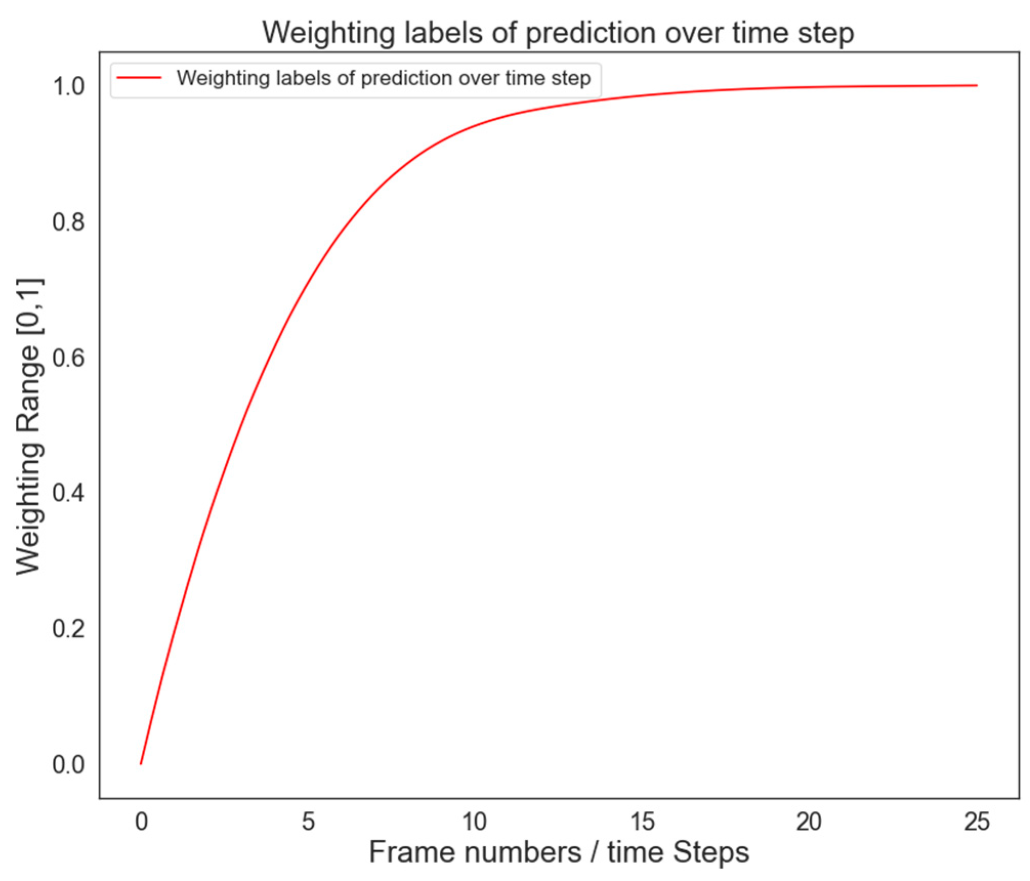
3.2. Prosposed Method

Inspired by [57], we use a pre-trained CNN model [22] to extract the features at frame level, and then a proposed version of PredNet [7], i.e., FWPredNet is used to predict the feature representation of the next video frame. Our idea is to condition the future frame predictions on predicted action class labels. The following section describes the functionality of the proposed FWPredNet architecture.
Figure 2. PredNet Architecture [7,58].
Remotesensing 14 00447 g002

3.2.1. Semantic Feature Extraction

Our proposed work considers the same network as GoogleNet [22]. However, we arranged the layers according to our needs by settling convolution with a stride size of two by adding seven pooling layers. The inception module was reduced to six layers. The datasets (HTA, KITTI, D2city) consisting of video images have different resolutions. In order to unify the training procedure, all images were resized to [224, 224], and fed in the classifier as an input. The original size of an image is shown as one eighth in resulting maps as [2048 × 3 × 3]. This helps us to detect even small objects with a fine-grained detection while maintaining a low computational load. For detection and recognition, we use the feature maps as the basis.
To address the aforementioned situations, we utilize the novel “Swish” activation function which was proposed in [23]. Suggested from the studies of Google Brain, where ϰ-input multiplies by sigmoid function, this is a reasonably simple feature (Swish activation function is demonstrated in Figure 3).
The mathematical definition [23] of ‘Swish’ is presented by using (1):
f ( x ) = x × s i g m o i d ( x )
Shown above is the Swish function which is graphically smooth; it doesn’t abruptly change its course, like RELU close to ϰ = 0. In contrast, it falls smoothly from 0 to less than 0, and soon thereafter rises. This information also indicates the non-monotonic nature of the function. Similarly, like RELU, this function does not persist as stable or unidirectional. Conforming to the experimental study performed in [23], the Swish function seems to operate in more complex data sets than RELU on deeper models. It performs with the same computational effectiveness, but better than RELU.

3.2.2. FW-PredNet Architecture

The basis of the theory of predictive coding is that the brain endlessly generates top-down predictions from bottom-up input. The representation at a higher level predicts the representation at its lower level. A difference between the predicted and actual representation causes an error in prediction. This error propagates to the higher levels to update their representations in order to attain an improved prediction. The process is repeated throughout the hierarchy until the prediction error reduces, or until bottom-up processes no longer transmit any “new” information (or unpredicted information) for updating hidden representations. Therefore, predictive coding is a computational mechanism by which the model recursively updates its internal representation of the visual input towards convergence.
The input to PredNet [7] is pixel-level image data and the authors utilized a four-layer architecture. Instead, we use the feature extracted from top layer of CNN which contains semantic information necessary for performing anomaly detection. In contrast to recognition in still images, motion and temporal aspects of videos play a significant role in action recognition. Accordingly, the majority of presently available state-of-the-art models use video pre-processing to acquire optical flow fields between contiguous video frames and models that can consume video sequences. Hence, rather than propagating errors at pixel level, we predict the error at feature level. Moreover, in order to make the prediction more robust, we engage classification unit (C) that is attached to the top of the representation layer. This unit consists of an encoder section and decoder section. The compilation of FWPredNet includes four core components which can be seen in Figure 4, in which, R , A ^ , A , E and C units denote representation unit, prediction, input, error and classification unit, respectively.
As referred to by Wen et al. [50], in FWPrednet the higher-level representation R l t where l is denoted as layer and t is denoted as time step predicts its low-level representation A ^ l 1 t via linear weighting W l , l 1 where the weights of layer l 1 , to layer l , are denoted as W . The prediction error E l 1 is the difference between A ^ l 1 t and R l t .
A ^ l 1 t = ( W l , l 1 ) T R l t   ( t )
E l 1 t = R l 1 ( t ) A ^ l 1 t
During the feedforward process, the prediction error on layer l 1 ,   E l 1 t , is propagated to upper layer l , in order to update its representation layer R l t ; thus, the prediction error is reduced with the updated representation. We can minimize E l 1 t , by defining losses as the sum of squared errors normalized by the variance of the representation σ l 1 2 as:
E l 1 t = 1 σ l 1 2 E l 1 t 2 2
The gradient of E l 1 t in contrast with R l t is given in Equation (5):
E l 1 t R l t = 2 σ l 1 2 W l , l 1 E l 1 t
To decrease E l 1 t , by using gradient descent, R l t is updated with an updating rate, α l , given in (6):
R l t + 1 = R l t α l ( E l 1 t R l t ) = R l t + 2 α l σ l 1 2 W l , l 1 E l 1 t
If the weights of feedback connections are the transpose of those of feedforward connections W l , l 1 = ( W l 1 , l ) T , it is possible to rewrite (6) as a feedforward operation, as in (7):
R l t + 1 = R l t + α l ( W l 1 , l ) T E l 1 t
This method involves forwarding the prediction error from layer l 1 to layer l , for updating the representation with an update rate of α l = 2 α l σ l 1 2 . During the feedback process, the top-down prediction is used to update representations at layer l ,   R l t in order to reduce prediction error E l t . In a similar way to the feedforward process, gradient descent is used to minimize error, where the gradient of E l t with respect to R l t is as in (8), and R l t is updated with an updating rate of β l , as in (9):
E l t R l t = 2 σ l 2 ( R l t A ^ l t )
R l t + 1 = R l t β l ( E l t R l t ) = ( 1 2 β l σ l 2 ) R l t + 2 β l σ l 2 A ^ l t
Let b l = 2 β l σ l 2 and (9) is rewritten as follows:
R l t + 1 = ( 1 b l ) R l t + b l A ^ l t  
Here, Equation (10) illustrates a feedback process where the representation at the higher layer R l + 1 t , caused top-down prediction A ^ l + 1 t , and impacts the lower layer representation R l t .
In Figure 2, we have included an additional ‘classifying unit’ which is composed of two ConvLSTM layers that convert the input R 2 1 into class probabilities shown in Figure 4. The decoder is made up of transposed convolution layers that upsample and transform the classes back to the image features, which are then fed back into the top down. The classification unit makes predictions at each in-coming frame. A weighted sum of these prediction scores is calculated and passed through the softmax function to get predicted class probability. In the first few frames of the video, the model does not have enough context to make any meaningful predictions and therefore the weighing over time is done using an exponential function, as shown as Figure 5. Notice how predictions in the first few frames are weighted low while weights for later predictions stabilize at 1.0.
First of all, R 0 1 and R 1 1 are all initialized as 0 in step one. Then, from the bottom layer zero, after convolution R 0 1 yields A ^ 0 1 as well as A 0 1 ,   A 0 1 and A ^ 0 1 . Later on, the convolution A 1 1 is produced by E 0 1 as input for the next layer of a same time step. The same principle applies to layer one, where R 1 1 generates A ^ 1 1 by convolution and E 1 1 is derived from subtractions between A ^ 1 1 as well as A 1 1 ,   A 1 1 and A ^ 1 1 . After convolution A 2 1 is produced by E 1 1 as input for the next layer of a same time step. As at layer two, R 2 1 produces A ^ 2 1 using convolution, whereas E 2 1 is derived via subtractions between A ^ 2 1 as well as A 2 1 ,   A 2 1 and A ^ 2 1 . This represents the conclusion of the bottom-up process. For the time step one at layer one, based on convolution LSTM,   R 2 1 and E 2 1 initialize R 2 2 at layer one for time step two. R 2 2 with E 1 1 and R 1 1 , output R 1 2 representing the bottom-up process. This bottom-up process occurs continuously throughout a time domain.
The encoder is composed of two ConvLSTM layers that convert the input R 2 1 into class probabilities. The decoder is made up of transposed convolution layers that upsample and transform the classes back to the image features, which later feed back into the top-down. The classification unit makes a prediction at each in-coming frame. A weighted sum of these prediction scores is calculated and passed through the softmax function to get predicted class probability. In the first few frames of the video, the model does not have enough context to make any meaningful predictions and therefore the weighting over time is performed by using an exponential function, as shown as Figure 5. Notice how predictions in the first few frames are weighted low while weights for later predictions stabilize at 1.0.
The number of classes recognized by classification unit (C) depends on the dataset, i.e., 2 classes for KITTI and D2City and 3 in case of HTA. These classes are interpreted as labels for future frame prediction. The encoder-decoder first transforms the output from representation unit R 2 1 into label class probabilities where the decoder transforms the output back to image modalities.

3.2.3. Network Training Parameters
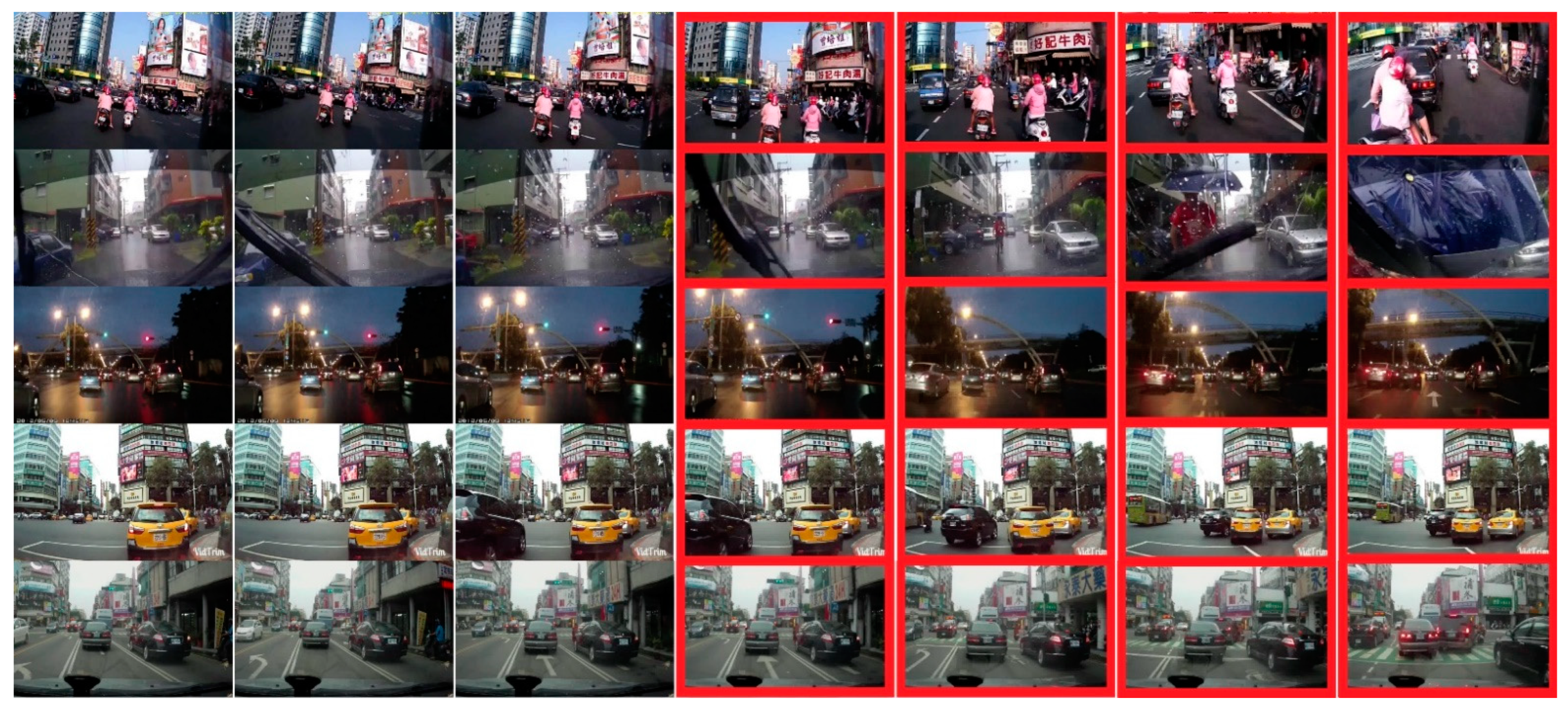
We use standard stochastic gradient descent (SGD) to train deep networks, with momentum set at 0.75 and weight decay at 0.001 in each case. Initial learning rate is 0.0057 andbatch size is 8. As soon as the validation loss reaches a saturation, 10x reduction of the learning rate is applied. Our FWPredNet model is trained using the action classification layer model for 40 epochs on the KITTI dataset. Our training or finetuning of moments uses only 10 plus epochs due to memory and time constraints. Models are all implemented in Pytorch using a 2080Ti.

3.3. Datasets

Our proposed method of analysis is conducted on three different large-scale HTA [8], KITTI [9], and D2city [10] dashcam videos datasets. Furthermore, Figure 6 shows the real video examples of these state-of-the-art datasets.

3.3.1. HTA

The collection of videos includes 1280 × 720 dashcam videos from cars recorded in New York and the Bay Area [8]. Videos have been excluded from this subset which are blurred or show visually degraded conditions. In brief, this dataset collection contains traffic videos (clear, cloudy, or semi-cloudy weather conditions), minimally appearing or blurred cars (due to large vehicles) also including traffic moving on the roads. This dataset is not noise-free or in other words, a little bit imperfect because of the flawed nature of data collection. For example, bumps and cracks on the road lead videos to have transient shakes. These features make the dataset more realistic and at the same time, more challenging to deal with anomalies. Videos lie in the standard driving conditions characterized in this dataset as vehicles that do not disturb a dashcam movement. The training set involves 286 regular traffic videos, an average length of 40 s and has a total count of 321,102 video frames.

3.3.2. KITTI

This selected dataset comprises 600 video frames (having a pixel value of 375 × 1242) [9] extracted at a minimum space distance of 20 m from the large-scale dataset of KITTI. The reported videos are from 5 different scenarios and are in comparatively low vehicle conditions, i.e., the road/path is often completely visible. Specific data was collected from the KITTI website and chosen for our work (including color-stereo photos, laser scans as Velodyne, information gathered by GPS).

3.3.3. D2city

D2city dataset [10] is a certain version, in which all videos and several scenarios of incidents are recorded, such as a motorcycle hitting a vehicle, or a car colliding another car, as shown in Figure 6. In addition, most videos are from different cities in Taiwan. These are usually busy streets with several moving items or objects and complex road signs/panels in a difficult driving vision. We noted the bounding boxes of vehicle, motorcycle, bike, person, and the time of accident manually for each video. 58 videos out of 678 are used for object detector training. The rest of the 620 files are randomly picked from 620 positive and 1130 negative clips, each consisting of 60 to 70 frames.

4. Experiments and Results

We evaluate the proposed approach on several datasets. In order to better understand what each module at each layer of our designed model does, we conducted extensive visualization experiments. In this section, we dedicate one paragraph to each of the evaluations on three different datasets (HTA, KITTI, D2city), estimating the average precision (AP), with a Figure and Table to aid in discussing the results.
One thing to mention is due to lack of dataset availability for anomaly anticipation, we have taken publicly available datasets and repurposed them for the anomaly anticipation. In case of HTA, we were able to classify the datasets in three different classes, i.e., Speeding Vehicle, Close Merge, and Accident whereas, in case of KITTI and D2City, we classify the datasets into two classes i.e., Close Merge and Accident. Some baseline methods for our proposed method’s comparison are given. We labeled the dataset with 3 different classes i.e., Accident, Close Merge, and Speeding Vehicle. We report top1 accuracy for abnormal event classification. Using a CNN, a sequence of images is passed that is subsequently encoded into feature maps. For abnormal event classification, the context feature is passed through a spatial pooling layer along with a fully connected layer followed by a multi-way SoftMax layer at the end. Since we are predicting frames (N + 10), the abnormal event is triggered immediately as soon as the frame is classified as one of the labeled classes. In this paper, we have introduced the FWPredNet framework for accident and anomaly anticipation, and outperformed the previous state-of-the-art by a better margin on the downstream tasks of classification accuracy on KITTI, D2city and HTA datasets.

4.1. Baseline

The baseline for our proposed method’s comparison is discussed in further subsections.

4.1.1. CGAN

Generative models can learn to predict dense optical flow from normal motion models, since an anomaly is described as an irregular motion [44]. For training purposes of optical flow, ground truth is evaluated by using OpenCV optical flow implementation. GAN can be generalized to a conditioned model (CGAN) with some additional information on either G or D for any further details such as class labels or other methodologies [60]. By feeding y to the discriminator D and generator G, the conditioning is carried out in an additional input layer. Noise prior pz(z) and y is combined via generator G, in a joint hidden representation. The framework of adversarial training offers exceptional stability in the format of this hidden representation. x and y are presented as input to a discriminator function in the discriminator D. The objective function for the condition is shown below in (11):
m i n G m i n D   V   ( D ,   G ) = F x ~ p d a t a ( x | y ) [ log D ( x ) ] + F z ~ p z ( z ) [ log ( 1 D ( z | y ) ) ]
In order to anticipate the optical flow between two sequential frames, the CGAN is trained [61]. Inputs to the generator are two RGB images concatenated depth wise, and usedto predict the optical flow. As one method for detecting abnormal motion is the usage of difference between the predicted optical flow by the generator and the actual optical flow of the ground truth. Using a sliding window, the difference is then averaged, and the frame is considered anomalous if it exceeds the threshold in any of the x or y components.

4.1.2. FlowNet

FlowNet [62] compared two architectures: FlowNet Simple and FlowNetCorr; both architectures are end-to-end approaches to learning. The system initially generates two images distinctly and then merges them in a correlation layer together and learns the higher representation. Additionally, multiplicative patch contrasts between two maps of functions are used with the correlation layer. More precisely, two multi-channel maps of m 1 and m 2 have the number of channels, height, and width as c ,   h and w . The correlation of two patches mentioned in the first map based on a1 and the second map a2 is then described as (12):
C ( A 1 , A 2 ) = o [ k , k ] × [ k , k ] m 1 ( a 1 + o ) , m 2 ( a 2 + o )
There are two trends described in the method [63] on neural network design for event cameras through recurrent (spiking) variants of EV-FlowNet and FireNet. In this study, authors propose a novel approach to event-based optical flow estimation using self-supervised learning (SSL), which stresses the ability of networks to integrate temporal data from successive slices of events. In the training pipeline, the self-supervised loss function was reformulated to improve its convexity.

4.2. Model Analysis

We design our experiments to analyze each part of our model as follows:
  • The last layer of CNN pre-trained on ImageNet is fine-tuned on HTA.
  • The last layer of CNN pre-trained on KITTI is fine-tuned on HTA.
  • Fix the weights of CNN pre-trained on ImageNet dataset and train the PredNet on HTA.
  • Fix the weights of CNN pre-trained on KITTI dataset and train the PredNet on HTA.
Experiments 1 and 2 are to examine the performance of CNN with different pre-trained weights and without temporal features. Experiment 3 and 4 are to exhibit how effective PredNet is with two pre-trained CNN models, respectively. Here, we present the results of our analysis for the HTA dataset. Using CNN pretrained on the KITTI dataset yields higher accuracy than using a model pre-trained in imageNet dataset, after fine-tuning the classification layer on HTA. The accuracy of the first result is 5.71% while other is 56.2%. This indicates the usage of features of the pre-trained model for object classification is not a good representation for traffic anomaly classification. If we add PredNet on both scenarios and train the PredNet from scratch on HTA, there is a significant boost in accuracy for both pre-trained CNN, with a 13% increase for the ImageNeT pre-trained CNN and more than 4% increase for the KITTI pre-trained one. This indicates that our proposed variation in FWPredNet is able to capture additional information from generated video sequences. Table 1 provides the classification accuracy for experimental results analysis of our model as follows.

4.2.1. Evaluation on HTA

Here, we discuss our model’s results compared with other baselines on the HTA dataset as described in Figure 7. We note that our model outperforms most of the cutting-edge approaches by a great margin, namely CGAN [60], FlowNet [62], and PredNet [7], by taking RGB frames only as an input. In addition to the RGB-frames, a two-stream model based on the convolution neural network explicitly contains optical flow which is used as the system input. Their model reaches a significantly higher rate of accuracy than that of our model, having only RGB frame inputs as in Table 2.

4.2.2. Evaluation on KITTI

We also conduct results on KITTI as an anomaly and anticipation results can be seen in Figure 8. In Table 3, a comparison of our system with state-of-the-art schemes is reported showing the identical results as extracted on the KITTI dataset. Our model only uses RGB frames as input and achieved 0.578 and 0.724 in Accident and Close Merge, respectively.

4.2.3. Evaluation on D2city

Compared to other models, our model performs better in both accident prediction and close merge detection on D2City detection, as shown in Figure 9. Our architecture uses optical flow as an input to the two-stream model. The model can achieve significantly higher accuracy than other models’ results as shown in Table 4 below.

5. Discussion

We implemented a model that is informally named as FWPredNet which outputs not only classification results, but also conditions future predictions on its previously labelled class labels. For all the experiments above, we report the top1 accuracy for supervised learning for action classification on KITTI, HTA and D2City in the rightmost column. The training and testing splits of KITTI, HTA, and D2City are presented. Table 2, Table 3 and Table 4 present top1 accuracy for action classification on the KITTI, HTA and D2City datasets.
Furthermore, we evaluated vanilla PredNet and compared it to our proposed model. Compared with traditional models, our model performs better in both Accident and Close Merge classes but struggles with the speeding vehicles because the learning ability of the model is sensitive to the continuity of the motion. Our model outperforms Flownet by 32.96%, with 7.4% in accident detection and marginally outperforms Flownet by 3.03% in HTA due to the type of the dataset and the learning ability of our model, which is sensitive to the continuity of the motion. Several of the presented techniques for extracting moving items are adopted in order to retrieve cues efficiently [50] and then represent these features as observations in our FWPredNet model by learning deep features. As compared with previous studies, Villegas et al. [40] predicted the future using both raw frames and their high-level representations, which is the frame’s corresponding human pose. However, this only works with static backgrounds and requires labelled pose information. Moreover, Vondrick et al. [13] extended this work and continued the tradition of encoding images at a higher level than pixels. In order to anticipate objects and actions, they used recognition algorithms on the predicted representation. In contrast, the PredNet [7] model that we extended and informally named as FWPredNet, learns directly from the pixel space and works with videos that have dynamic backgrounds and real-world settings. Moreover, this model is a type of neuroscientific framework that can learn features at different hierarchical levels without being specifically tuned to do so.
Parameter comparison of baseline (CGAN, FlowNet and PredNet) with our proposed FWPredNet is shown in Table 5. below. The vanilla Prednet model is approximately 3.9 M parameters less than the FWPrednet model, but it performs significantly better in every class and dataset. It is a compromise we have to strike to extract better results from Prednet’s classification performance. Hence, we adopted a kind of trade-off for “accuracy over computational cost” which will be interesting to explore for better classification performance in future work.

6. Conclusions and Future Work

  • In this paper, we have introduced the FWPredNet framework for accident and anomaly anticipation, and outperformed the previous state-of-the-art by a better margin on the downstream tasks of classification accuracy on KITTI, D2city and HTA datasets.
  • It can be deduced that our proposed variation in FWPredNet is able to capture additional information from generated video sequences while we train the PredNet from scratch on the given dataset.
  • We evaluated vanilla PredNet [7] then compared it to our FWPredNet model. Compared with traditional models (CGAN, Flownet, PredNet), FWPredNet performs better in both Accident and Close Merge classes. One limitation of the test performance is that it struggles with speeding vehicles because the learning ability of the model is sensitive to the continuity of motion but still achieves better results compared with the rest of the three methods.
  • Finally, on the engineering front, the current implementation of the FWPredNet takes very long time to train, and work can be done towards more efficient usage of GPUs. The computational cost of FWPredNet is 3.9M more than the vanilla PredNet but we accepted it as trade-off for “accuracy over computational cost”. A successor to FWPredNet can be designed, which does not have the aforementioned limitations and is faster in implementation of the proposed model.

Author Contributions

Conceptualization, W.R. and G.C.; methodology, W.R.; software S. and W.R.; validation, A.A.; formal analysis, W.R.; investigation, G.C.; resources, A.A. and A.U.; data curation, W.R. and G.C.; writing—original draft preparation, W.R.; writing—review and editing, G.C., J.A.B. and S.; visualization, A.U.; supervision, G.C.; project administration, W.R. and A.U.; funding acquisition, G.C. All authors have read and agreed to the published version of the manuscript.

Funding

This work is supported by the National Natural Science Foundation of China (No. 62176035), the Science and Technology Research Program of Chongqing Municipal Education Commission under Grant (No.KJZD-K202100606).

Institutional Review Board Statement

Not applicable.

Informed Consent Statement

Not applicable.

Data Availability Statement

Not applicable.

Acknowledgments

The authors would like to thank the editor and anonymous reviewers for their valuable comments on this paper.

Conflicts of Interest

The authors declare no conflict of interest.

References

  1. Shirazi, M.S.; Morris, B.T. Looking at Intersections: A Survey of Intersection Monitoring, Behavior and Safety Analysis of Recent Studies. IEEE Trans. Intell. Transp. Syst. 2017, 18, 4–24. [Google Scholar] [CrossRef]
  2. Yuan, Y.; Fang, J.; Wang, Q. Online Anomaly Detection in Crowd Scenes via Structure Analysis. IEEE Trans. Cybern. 2015, 45, 548–561. [Google Scholar] [CrossRef] [PubMed]
  3. Cheng, K.-W.; Chen, Y.-T.; Fang, W.-H. Gaussian Process Regression-Based Video Anomaly Detection and Localization with Hierarchical Feature Representation. IEEE Trans. Image Process. 2015, 24, 5288–5301. [Google Scholar] [CrossRef] [PubMed]
  4. Zhao, M.; Chen, J. A Review of Methods for Detecting Point Anomalies on Numerical Dataset. In Proceedings of the 2020 IEEE 4th Information Technology, Networking, Electronic and Automation Control Conference (ITNEC), Chongqing, China, 12–14 June 2020; pp. 559–565. [Google Scholar]
  5. Janai, J.; Güney, F.; Behl, A.; Geiger, A. Computer vision for autonomous vehicles: Problems, datasets and state of the art. In Foundations and Trends® in Computer Graphics and Vision; Now Publishers: Boston, MA, USA, 2021; Volume 12, pp. 1–308. [Google Scholar]
  6. Muhammad, K.; Ullah, A.; Lloret, J.; Del Ser, J.; de Albuquerque, V.H.C. Deep Learning for Safe Autonomous Driving: Current Challenges and Future Directions. IEEE Trans. Intell. Transp. Syst. 2020, 22, 4316–4336. [Google Scholar] [CrossRef]
  7. Lotter, W.; Kreiman, G.; Cox, D. Deep predictive coding networks for video prediction and unsupervised learning. arXiv 2016, arXiv:1605.0810. [Google Scholar]
  8. Yu, F.; Xian, W.; Chen, Y.; Liu, F.; Liao, M.; Madhavan, V.; Darrell, T. Bdd100k: A diverse driving video database with scalable annotation tooling. arXiv 2018, arXiv:1805.04687. [Google Scholar]
  9. Geiger, A.; Lenz, P.; Urtasun, R. Are we ready for autonomous driving? The KITTI vision benchmark suite. In Proceedings of the IEEE Conference on Computer Vision and Pattern Recognition (CVPR), Providence, RI, USA, 16–21 June 2012; pp. 3354–3361. [Google Scholar] [CrossRef]
  10. Che, Z.; Li, G.; Li, T.; Jiang, B.; Shi, X.; Zhang, X.; Ye, J. D2City: A Large-Scale Dashcam Video Dataset of Diverse Traffic Scenarios. arXiv 2019, arXiv:1904.01975. [Google Scholar]
  11. Wang, Y.; Gao, Z.; Long, M.; Wang, J.; Yu, P.S. Predrnn++: Towards A resolution of the deep-in-time dilemma in spatiotemporal predictive learning. In Proceedings of the International Conference on Machine Learning, Stockholm, Sweden, 10–15 July 2018. [Google Scholar]
  12. Finn, C.; Goodfellow, I.; Levine, S. Unsupervised learning for physical interaction through video prediction. In Advances in Neural Information Processing Systems 29; Lee, D.D., Sugiyama, M., Luxburg, U.V., Guyon, I., Garnett, R., Eds.; Curran Associates, Inc.: Red Hook, NY, USA, 2016; pp. 64–72. [Google Scholar]
  13. Vondrick, C.; Pirsiavash, H.; Torralba, A. Anticipating the Future by Watching Unlabeled Video. 2015. Available online: http://www.cs.columbia.edu/~vondrick/prediction/paper.pdf (accessed on 15 December 2021).
  14. Sutskever, I.; Vinyals, O.; Le, Q.V. Sequence to sequence learning with neural networks. In Advances in Neural Information Processing Systems; Curran Associates, Inc.: Red Hook, NY, USA, 2014; pp. 3104–3112. [Google Scholar]
  15. Hochreiter, S.; Schmidhuber, J. Long short-term memory. Neural Comput. 1997, 9, 1735–1780. [Google Scholar] [CrossRef] [PubMed]
  16. Riaz, W.; Azeem, A.; Chenqiang, G.; Yuxi, Z.; Saifullah; Khalid, W. YOLO Based Recognition Method for Automatic License Plate Recognition. In Proceedings of the 2020 IEEE International Conference on Advances in Electrical Engineering and Computer Applications (AEECA), Dalian, China, 25–27 August 2020; pp. 87–90. [Google Scholar]
  17. Bao, W.; Yu, Q.; Kong, Y. Uncertainty-based traffic accident anticipation with spatio-temporal relational learning. In Proceedings of the 28th ACM International Conference on Multimedia, Seattle, WA, USA, 16–18 October 2020; pp. 2682–2690. [Google Scholar]
  18. Carreira, J.; Zisserman, A. Quo vadis, action recognition? A new model and the kinetics dataset. In Proceedings of the IEEE Conference on Computer Vision and Pattern Recognition, Honolulu, HI, USA, 21–26 July 2017; pp. 6299–6308. [Google Scholar]
  19. Zhu, J.; Zhu, Z.; Zou, W. End-to-end video-level representation learning for action recognition. In Proceedings of the 24th International Conference on Pattern Recognition (ICPR), Beijing, China, 20–24 August 2018; pp. 645–650. [Google Scholar]
  20. Wang, L.; Xiong, Y.; Wang, Z.; Qiao, Y.; Lin, D.; Tang, X.; Van Gool, L. Temporal Segment Networks: Towards Good Practices for Deep Action Recognition. In Proceedings of the European Conference on Computer Vision (ECCV), Amsterdam, The Netherlands, 8–16 October 2016; Leibe, B., Matas, J., Sebe, N., Welling, M., Eds.; Springer: Cham, Switzerland, 2016; pp. 20–36. [Google Scholar]
  21. Sevilla-Lara, L.; Liao, Y.; Güney, F.; Jampani, V.; Geiger, A.; Black, M.J. On the integration of optical flow and action recognition. In Proceedings of the German Conference on Pattern Recognition, Stuttgart, German, 9–12 October 2018; Springer: Cham, Switzerland, 2018; pp. 281–297. [Google Scholar]
  22. Szegedy, C.; Liu, W.; Jia, Y. Going deeper with convolutions. In Proceedings of the IEEE Conference on Computer Vision and Pattern Recognition, Boston, MA, USA, 7–12 June 2015; pp. 1–9. [Google Scholar]
  23. Ramachandran, P.; Zoph, B.; Le, Q.V. Swish: A self-gated activation function. arXiv 2017, arXiv:1710.059417. [Google Scholar]
  24. Kamijo, S.; Matsushita, Y.; Ikeuchi, K.; Sakauchi, M. Traffic monitoring and accident detection at intersections. IEEE Trans. Intell. Transp. Syst. 2000, 1, 108–118. [Google Scholar] [CrossRef]
  25. Rojas, J.C.; Crisman, J.D. Vehicle detection in color images. In Proceedings of the Conference on Intelligent Transportation Systems, Boston, MA, USA, 12 November 1997. [Google Scholar]
  26. Leibe, B.; Schindler, K.; Cornelis, N.; Van Gool, L. Coupled object detection and tracking from static cameras and moving vehicles. IEEE Trans. Pattern Anal. Mach. Intell. 2008, 30, 1683–1698. [Google Scholar] [CrossRef] [PubMed]
  27. Lai, A.H.S.; Yung, N.H.C. A video-based system methodology for detecting red light runners. In Proceedings of the IAPR Workshop on Machine Vision Applications, Chiba, Japan, 17–19 November 1998; pp. 23–26. [Google Scholar]
  28. Fatima, M.; Khan, M.U.K.; Kyung, C.M. Global feature aggregation for accident anticipation. arXiv 2020, arXiv:2006.08942. [Google Scholar]
  29. Thajchayapong, S.; Garcia-Trevino, E.S.; Barria, J.A. Distributed Classification of Traffic Anomalies Using Microscopic Traffic Variables. IEEE Trans. Intell. Transp. Syst. 2012, 14, 448–458. [Google Scholar] [CrossRef]
  30. Ikeda, H.; Kaneko, Y.; Matsuo, T.; Tsuji, K. Abnormal incident detection system employing image processing technology. In Proceedings of the 1999 IEEE/IEEJ/JSAI International Conference on Intelligent Transportation Systems (Cat. No. 99TH8383), Tokyo, Japan, 5–8 October 1999; pp. 748–752. [Google Scholar]
  31. Michalopoulos, P.; Jacobson, R. Field Implementation and Testing of Machine Vision Based Incident Detection System. In Proceedings of the Pacific Rim TransTech Conference: Volume I: Advanced Technologies, Washington, DC, USA, 25–28 July 1993; pp. 1–7. [Google Scholar]
  32. Ki, Y.K.; Kim, J.W.; Baik, D.K. A traffic accident detection model using metadata registry. In Proceedings of the Fourth International Conference on Software Engineering Research, Management and Applications, IEEE (SERA'06), Seattle, WA, USA, 9–11 August 2006; pp. 255–259. [Google Scholar]
  33. Wei, J.; Zhao, J.; Zhao, Y.; Zhao, Z. Unsupervised anomaly detection for traffic surveillance based on background modeling. In Proceedings of the IEEE Conference on Computer Vision and Pattern Recognition Workshops, Salt Lake City, UT, USA, 18–22 June 2018; pp. 129–136. [Google Scholar]
  34. Liu, X.; Zhang, S.; Huang, Q.; Gao, W. Ram: A region-aware deep model for vehicle reidentification. In Proceedings of the 2018 IEEE International Conference on Multimedia and Expo (ICME), San Diego, CA, USA, 23–27 July 2018; pp. 1–6. [Google Scholar]
  35. Schlegl, T.; Seeböck, P.; Waldstein, S.M.; Schmidt-Erfurth, U.; Langs, G. Unsupervised anomaly detection with generative adversarial networks to guide marker discovery. In Proceedings of the International Conference on Information Processing in Medical Imaging, Boone, NC, USA, 25–30 June 2017; pp. 146–157. [Google Scholar]
  36. Bochinski, E.; Senst, T.; Sikora, T. Extending IOU based multiobject tracking by visual information. In Proceedings of the 15th IEEE International Conference on Advanced Video and Signal Based Surveillance (AVSS) IEEE, Auckland, New Zealand, 27–30 November 2018; pp. 1–6. [Google Scholar]
  37. Dogru, N.; Subasi, A. Traffic accident detection by using machine learning methods. In Proceedings of the Third International Symposium on Sustainable Development (ISSD’12), Sarajevo, Bosia and Herzegovina, 31 May–1 June 2012; p. 467. [Google Scholar]
  38. Yun, K.; Jeong, H.; Yi, K.M.; Kim, S.W.; Choi, J.Y. Motion Interaction Field for Accident Detection in Traffic Surveillance Video. In Proceedings of the 22nd International Conference on Pattern Recognition, Stockholm, Sweden, 24–28 August 2014; pp. 3062–3067. [Google Scholar] [CrossRef]
  39. Srivastava, N.; Mansimov, E.; Salakhutdinov, R. Unsupervised learning of video representations using lstms. In Proceedings of the 32nd International Conference on Machine Learning, Lille, France, 7–9 July 2015. [Google Scholar]
  40. Villegas, R.; Yang, J.; Zou, Y.; Sohn, S.; Lin, X.; Lee, H. Learning to generate long-term future via hierarchical prediction. In Proceedings of the 34th International Conference on Machine Learning, Sydney, NSW, Australia, 6–11 August 2017. [Google Scholar]
  41. Morris, B.; Doshi, A.; Trivedi, M. Lane change intent prediction for driver assistance: On-road design and evaluation. In Proceedings of the IEEE Intelligent Vehicles Symposium (IV), Baden-Baden, Germany, 5–9 June 2011; pp. 895–901. [Google Scholar] [CrossRef]
  42. Jain, A.; Koppula, H.S.; Raghavan, B.; Soh, S.; Saxena, A. Car that Knows Before You Do: Anticipating Maneuvers via Learning Temporal Driving Models. In Proceedings of the IEEE International Conference on Computer Vision (ICCV), Santiago, Chile, 7–13 December 2015; pp. 3182–3190. [Google Scholar] [CrossRef]
  43. Santhosh, K.K.; Dogra, D.P.; Roy, P.P. Anomaly detection in road traffic using visual surveillance: A survey. ACM Comput. Surv. (CSUR) 2020, 53, 1–26. [Google Scholar] [CrossRef]
  44. Pathak, D.; Sharang, A.; Mukerjee, A. Anomaly Localization in Topic-Based Analysis of Surveillance Videos. In Proceedings of the IEEE Winter Conference on Applications of Computer Vision, Waikoloa, HI, USA, 5–9 January 2015; pp. 389–395. [Google Scholar] [CrossRef]
  45. Sultani, W.; Chen, C.; Shah, M. Real-World Anomaly Detection in Surveillance Videos. In Proceedings of the IEEE Computer Society Conference on Computer Vision and Pattern Recognition, Salt Lake City, UT, USA, 18–22 June 2018; pp. 6479–6488. [Google Scholar]
  46. Lee, S.; Kim, H.G.; Ro, Y.M. STAN: Spatio-Temporal Adversarial Networks for Abnormal Event Detection. In Proceedings of the IEEE International Conference on Acoustics, Speech and Signal Processing (ICASSP), Calgary, AB, Canada, 15–20 April 2018; pp. 1323–1327. [Google Scholar] [CrossRef]
  47. Scharwächter, T.; Enzweiler, M.; Franke, U.; Roth, S. Efficient Multi-cue Scene Segmentation. In Proceedings of the DAGM German Conference on Pattern Recognition, Saarbrücken, Germany, 3–6 September 2013; Volume 8142, pp. 435–445. [Google Scholar] [CrossRef]
  48. Zhong, J.; Cangelosi, A.; Zhang, X.; Ogata, T. AFA-PredNet: The Action Modulation Within Predictive Coding. In Proceedings of the International Joint Conference on Neural Networks (IJCNN), Rio de Janeiro, Brazil, 8–13 July 2018; pp. 1–8. [Google Scholar] [CrossRef]
  49. Zhong, J.; Ogata, T.; Cangelosi, A. Encoding longer-term contextual multi-modal information in a predictive coding model. arXiv 2018, arXiv:1804.06774. [Google Scholar]
  50. Wen, H.; Han, K.; Shi, J.; Zhang, Y.; Culurciello, E.; Liu, Z. Deep predictive coding network for object recognition. In Proceedings of the 35th International Conference on Machine Learning, Stockholm, Sweden, 10–15 July 2018. [Google Scholar]
  51. Scharwächter, T.; Enzweiler, M.; Franke, U.; Roth, S. Stixmantics: A medium-level model for real-time semantic scene understanding. In European Conference on Computer Vision; Springer: Cham, Switzerland, 2014. [Google Scholar]
  52. Leibe, B.; Cornelis, N.; Cornelis, K.; Van Gool, L. Dynamic 3D Scene Analysis from a Moving Vehicle. In Proceedings of the 2007 IEEE Conference on Computer Vision and Pattern Recognition, Minneapolis, MN, USA, 17–22 June 2007; pp. 1–8. [Google Scholar]
  53. Brostow, G.J.; Shotton, J.; Fauqueur, J.; Cipolla, R. Segmentation and recognition using structure from motion point clouds. In Proceedings of the European Conference on Computer Vision, Marseille, France, 12–18 October 2008; Volume 5302, pp. 44–57. [Google Scholar]
  54. Cordts, M.; Omran, M.; Scharwächter, T.; Rehfeld, T.; Enzweiler, M.; Benenson, R.; Franke, U.; Roth, S.; Schiele, B. The cityscapes dataset for Semantic Urban Scene Understanding. In Proceedings of the IEEE Conference on Computer Vision and Pattern Recognition (CVPR), Las Vegas, NV, USA, 6 April 2016; pp. 3213–3223. [Google Scholar]
  55. Chan, F.-H.; Chen, Y.-T.; Xiang, Y.; Sun, M. Anticipating Accidents in Dashcam Videos. In Proceedings of the 13th Asian Conference on Computer Vision, Taipei, Taiwan, 20–24 November 2016; Springer: Cham, Switzerland, 2017; pp. 136–153. [Google Scholar] [CrossRef]
  56. Shi, X.; Chen, Z.; Wang, H.; Yeung, D.; Wong, W.; Woo, W. Convolutional LSTM network: A machine learning approach for precipitation nowcasting. In Advances in Neural Information Processing Systems; Curran Associates, Inc.: Red Hook, NY, USA, 2015. [Google Scholar]
  57. Huang, X.; Mousavi, H.; Roig, G. Predictive Coding Networks Meet Action Recognition. In Proceedings of the 2020 IEEE International Conference on Image Processing (ICIP), Abu Dhabi, United Arab Emirates, 25–28 October 2020; pp. 793–797. [Google Scholar]
  58. Rane, R.P.; Szügyi, E.; Saxena, V.; Ofner, A.; Stober, S. Prednet and Predictive Coding: A Critical Review. In Proceedings of the 2020 International Conference on Multimedia Retrieval, Dublin, Ireland, 8–11 June 2020; pp. 233–241. [Google Scholar]
  59. Singh, H.; Hand, E.M.; Alexis, K. Anomalous Motion Detection on Highway Using Deep Learning. In Proceedings of the 2020 IEEE International Conference on Image Processing (ICIP), Abu Dhabi, United Arab Emirates, 25–28 October 2020; pp. 1901–1905. [Google Scholar]
  60. Mirza, M.; Osindero, S. Conditional Generative Adversarial Nets. arXiv 2014, arXiv:1411.1784. [Google Scholar]
  61. Ravanbakhsh, M.; Sangineto, E.; Nabi, M.; Sebe, N. Training Adversarial Discriminators for Cross-Channel Abnormal Event Detection in Crowds. In Proceedings of the IEEE Winter Conference on Applications of Computer Vision (WACV), Waikoloa, HI, USA, 7–11 January 2019; pp. 1896–1904. [Google Scholar] [CrossRef]
  62. Fischer, P.; Dosovitsky, A. FlowNet: Learning Optical Flow with Convolutional Networks. arXiv 2015, arXiv:1504.06852v2. [Google Scholar]
  63. Hagenaars, J.J.; Paredes-Vallés, F. Self-Supervised Learning of Event-Based Optical Flow with Spiking Neural Networks. arXiv 2021, arXiv:2106.01862v. [Google Scholar]
Figure 1. Snapshots of certain specialized strategies for identifying anomalies in a summarized manner. The images are taken from [43]. (a) Motion Interaction Field (MIF) [38] accident detection. (b) The topic-based model anomaly detection [44]. A car that has crossed the stop line appears on top of the row, a middle row is a hybrid, and a vehicle taking an odd turn is on the bottom of the row. (c) Multi-instance learning (MIL) anomaly detection in the real-time example [45]. The use of an anomaly ranking determines the detection of anomalies. (d) A vehicle on a walkway is identified with the STAN method [46]: as the top row is generator anomaly visualization, and the lower row represents the discriminator’s anomaly visualization [47].
Remotesensing 14 00447 g001
Figure 3. Graphical representation of Swish activation function.
Remotesensing 14 00447 g003
Figure 4. Left: FWPredNet architecture for our proposed model, in which each time step consists of five important components— A the input unit,   A ^ the prediction unit, R the representation unit, and E the error unit. Right: architecture of classification unit C .
Remotesensing 14 00447 g004
Figure 5. Weighting of label prediction over time step.
Remotesensing 14 00447 g005
Figure 6. Some real video frames examples of three different large-scale datasets we are using in our experiments. These images are taken from [8,9,10,59].
Remotesensing 14 00447 g006
Figure 7. Playing from left to right given the above illustration shows successful anomaly and accident anticipation in HTA dashcam videos dataset.
Remotesensing 14 00447 g007
Figure 8. Playing from left to right given the above illustration shows successful anomaly and accident anticipation in KITTI dashcam videos dataset.
Remotesensing 14 00447 g008
Figure 9. Playing from left to right given the above illustration shows successful anomaly and accident anticipation in D2city dashcam videos dataset.
Remotesensing 14 00447 g009
Table 1. Experiment result analysis of our FWPredNet on the HTA. CNN has two versions—pre-trained on ImageNet or KITTI. FWPredNet is trained on HTA dataset.
Model StructurePretrained OnFineTune/TrainingAccuracy
CNNFWPredNetCNNFWPredNet
CNNImageNet Classification Layer 5.71%
CNNKITTI Classification Layer 56.2%
CNN + PredNetImageNet Fixed weightsFrom scratch18.44%
CNN + PredNetKITTISubset of KITTIFixed weightsFrom scratch60.3%
Table 2. Comparison between CGAN, Flownet, PredNet and our FWPredNet model for HTA datasets.
ActionCGANFlowNetPredNetFWPredNet
Speeding Vehicle0.6080.6230.490.629
Accident0.6070.6570.550.675
Close Merge0.4220.5310.190.651
Table 3. Shows the resulted comparison between CGAN, Flownet, Prednet our FWPredNet model for KITTI datasets.
ACTIONCGANFlowNetPredNetFWPredNet
Accident0.4390.5410.380.578
Close Merge0.5260.6850.450.724
Table 4. Comparison between CGAN, Flownet, PredNet and our FWPredNet model for D2city dataset.
ActionCGANFlowNetPredNetFWPredNet
Accident0.4390.5410.380.718
Close Merge0.5260.6850.470.704
Table 5. Parameter comparison for computational cost for FWPredNet with our baseline.
ModelTraining VRAM (GB)Model Parameters (in Millions)Batch Size
Resolution:224PredNet [7]3.87.28
CGAN [60]10.1454
FlowNet [62]9.5394
FW-PredNet5.311.18
Publisher’s Note: MDPI stays neutral with regard to jurisdictional claims in published maps and institutional affiliations.

