
Integrated Preprocessing of Multitemporal Very-High-Resolution Satellite Images via Conjugate Points-Based Pseudo-Invariant Feature Extraction


Abstract
:
1. Introduction
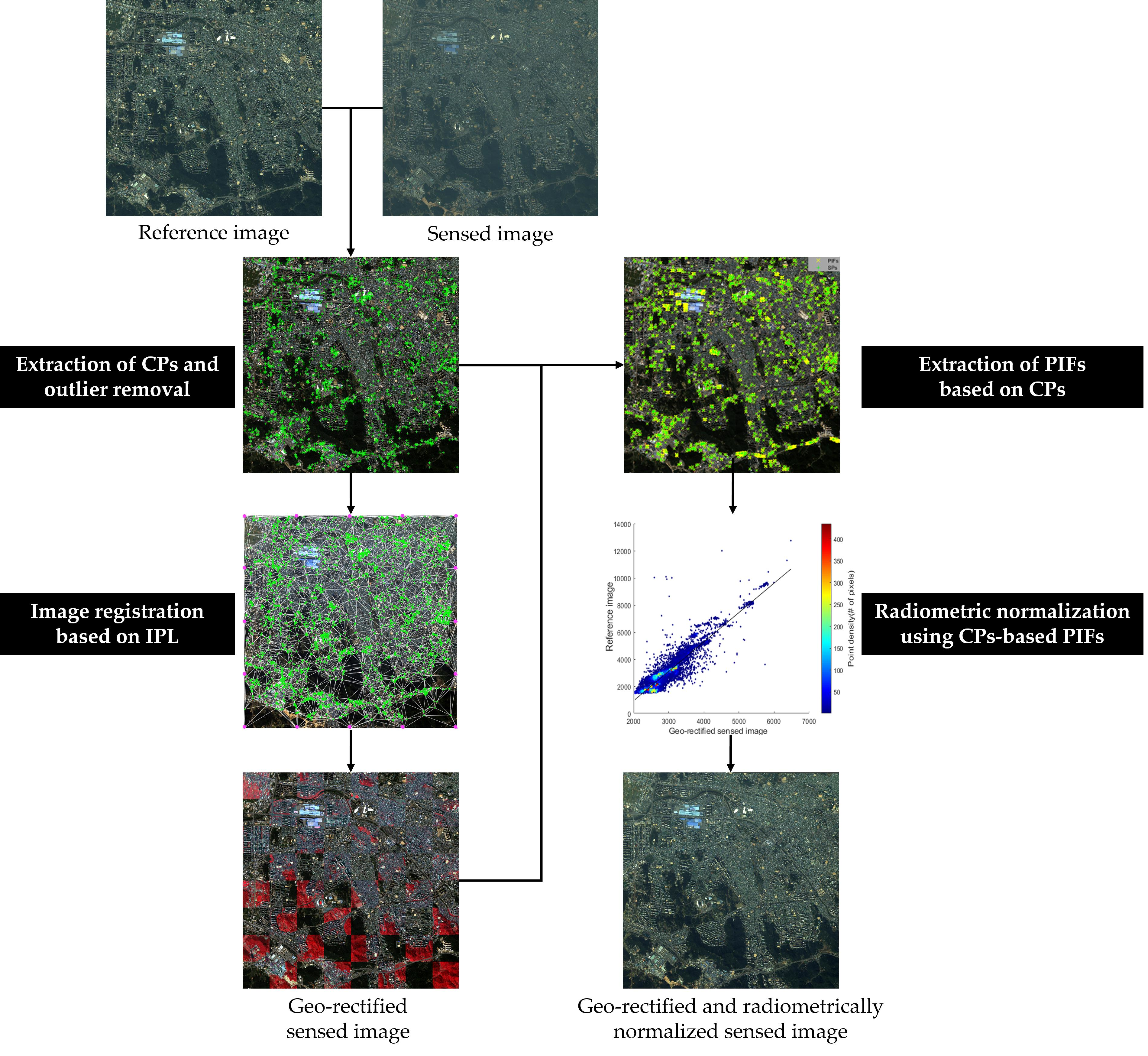
2. Methodology
2.1. Image Registration Using CPs Extracted from the SURF Algorithm and Outlier Removal
2.2. Extraction of Initial PIFs from CPs on Non-Vegetation Areas
2.3. Extraction of PIFs Using Z-Score Image and Region Growing Algorithm
2.4. Relative Radiometric Normalization Using PIFs Based on CPs
3. Dataset Description and Experimental Design
3.1. Dataset Description
3.2. Method for the Analysis of Experimental Results
- Assessment 1: image registration accuracy of the proposed method.
- Assessment 2: overall characteristics and quality of the PIFs extracted by the proposed method.
- Assessment 3: performance analysis of the proposed method through comparative analysis with other RRN algorithms.
4. Experimental Results
4.1. Image Registration Results
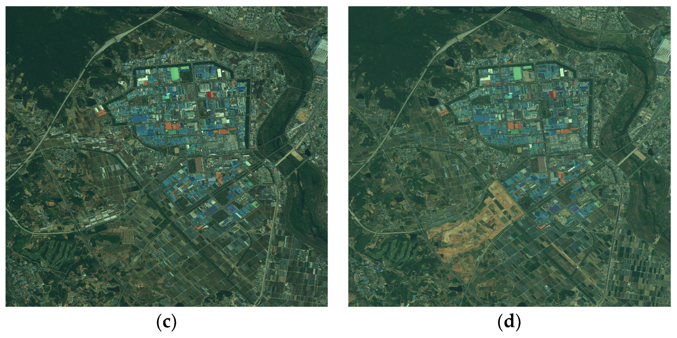
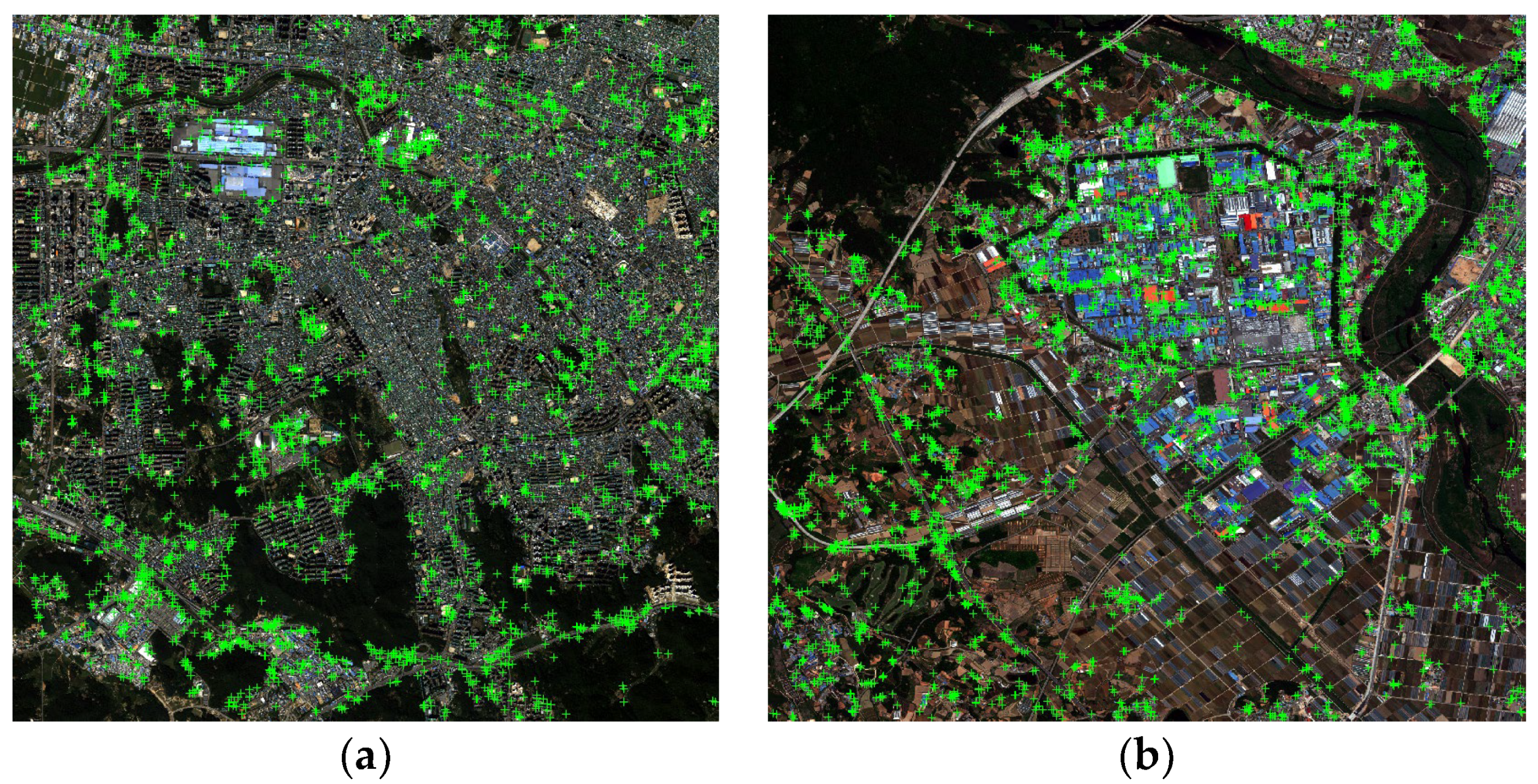
4.2. PIFs Extraction Result
4.3. Analysis of PIFs Characteristics and Quality
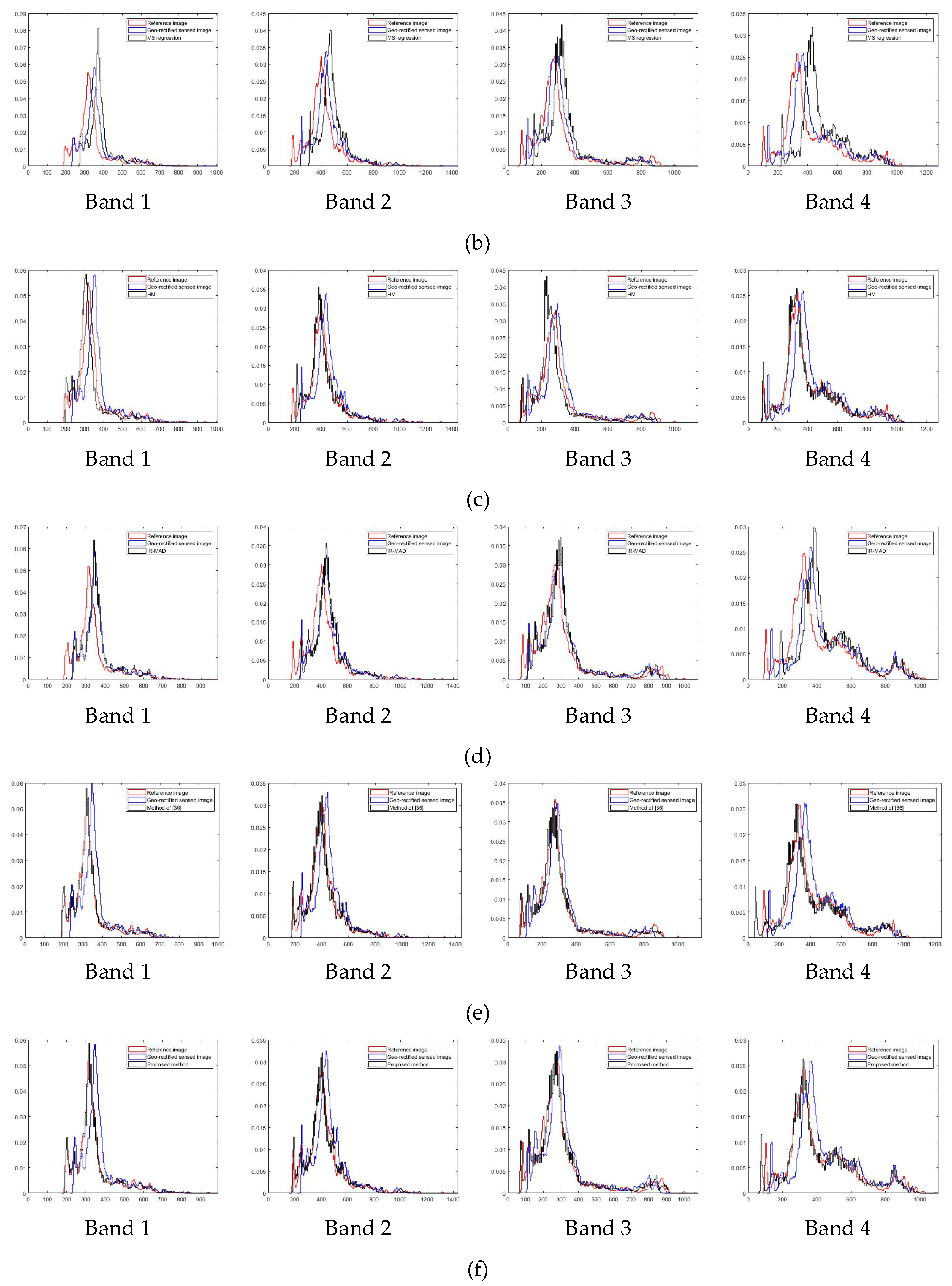
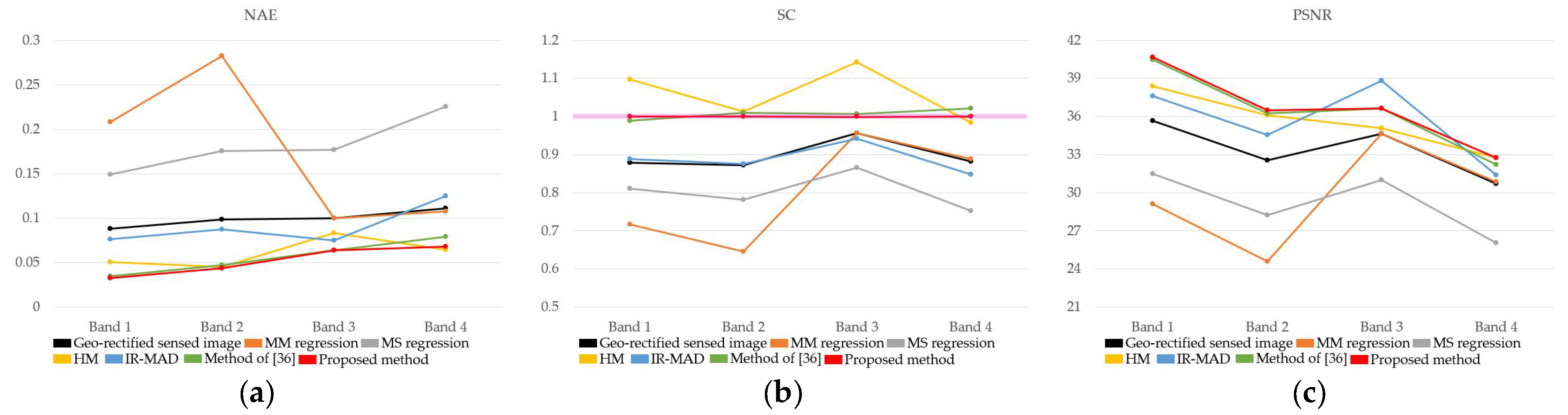
4.4. Relative Radiometric Normalization Performance
5. Discussion
6. Conclusions
Author Contributions
Funding
Conflicts of Interest
References
- Han, Y.; Bovolo, F.; Bruzzone, L. An approach to fine coregistration between very high resolution multispectral images based on registration noise distribution. IEEE Trans. Geosci. Remote Sens. 2015, 53, 6650–6662. [Google Scholar] [CrossRef]
- Li, C.; Xiong, H. A geometric and radiometric simultaneous correction model (GRSCM) framework for high-accuracy remotely sensed image preprocessing. Photogramm. Eng. Remote Sens. 2017, 83, 621–632. [Google Scholar] [CrossRef]
- Canty, M.J.; Nielsen, A.A.; Schmidt, M. Automatic radiometric normalization of multitemporal satellite imagery. Remote Sens. Environ. 2004, 91, 441–451. [Google Scholar] [CrossRef] [Green Version]
- Johnson, R.D.; Kasischke, E.S. Change vector analysis: A technique for the multispectral monitoring of land cover and condition. Int. J. Remote Sens. 1998, 19, 411–426. [Google Scholar] [CrossRef]
- Bruzzone, L.; Bovolo, F. A novel framework for the design of change-detection systems for very-high-resolution remote sensing images. Proc. IEEE 2013, 101, 609–630. [Google Scholar] [CrossRef]
- Chen, X.; Vierling, L.; Deering, D. A simple and effective radiometric correction method to improve landscape change detection across sensors and across time. Remote Sens. Environ. 2005, 98, 63–79. [Google Scholar] [CrossRef]
- Afek, Y.; Brand, A. Mosaicking of orthorectified aerial images. Photogramm. Eng. Remote Sens. 1998, 64, 115–124. [Google Scholar]
- Solano-Correa, Y.T.; Bovolo, F.; Bruzzone, L. Generation of homogeneous VHR time series by nonparametric regression of multisensor bitemporal images. IEEE Trans. Geosci. Remote Sens. 2019, 57, 7579–7593. [Google Scholar] [CrossRef]
- Huo, C.; Pan, C.; Huo, L.; Zhou, Z. Multilevel SIFT matching for large-size VHR image registration. IEEE Geosci. Remote Sens. Lett. 2011, 9, 171–175. [Google Scholar] [CrossRef]
- Lee, I.H.; Choi, T.S. Accurate registration using adaptive block processing for multispectral images. IEEE Trans. Circuits Syst. Video Technol. 2013, 23, 1491–1501. [Google Scholar] [CrossRef]
- Toutin, T. Geometric processing of remote sensing images: Models, algorithms and methods. Int. J. Remote Sens. 2004, 25, 1893–1924. [Google Scholar] [CrossRef]
- Zitová, B.; Flusser, J. Image registration methods: A survey. Image Vis. Comput. 2003, 21, 977–1000. [Google Scholar] [CrossRef] [Green Version]
- Hong, G.; Zhang, Y. Wavelet-based image registration technique for high-resolution remote sensing images. Comput. Geosci. 2008, 34, 1708–1720. [Google Scholar] [CrossRef]
- Bentoutou, Y.; Taleb, N.; Kpalma, K.; Ronsin, J. An automatic image registration for applications in remote sensing. IEEE Trans. Geosci. Remote Sens. 2005, 43, 2127–2137. [Google Scholar] [CrossRef]
- Kennedy, R.E.; Cohen, W.B. Automated designation of tie-points for image-to-image coregistration. Int. J. Remote Sens. 2003, 24, 3467–3490. [Google Scholar] [CrossRef] [Green Version]
- Feng, R.; Du, Q.; Li, X.; Shen, H. Robust registration for remote sensing images by combining and localizing feature- and area-based methods. ISPRS J. Photogramm. Remote Sens. 2019, 19, 15–26. [Google Scholar] [CrossRef]
- Wang, S.; Quan, D.; Liang, X.; Ning, M.; Guo, Y.; Jiao, L. A deep learning framework for remote sensing image registration. ISPRS J. Photogramm. Remote Sens. 2018, 145, 148–164. [Google Scholar] [CrossRef]
- Chen, H.M.; Arora, M.K.; Varshney, P.K. Mutual information-based image registration for remote sensing data. Int. J. Remote Sens. 2003, 24, 3701–3706. [Google Scholar] [CrossRef]
- Okorie, A.; Makrogiannis, S. Region-based image registration for remote sensing imagery. Comput. Vis. Image Underst. 2019, 189, 102825. [Google Scholar] [CrossRef]
- Ye, Y.; Shan, J. A local descriptor based registration method for multispectral remote sensing images with non-linear intensity differences. ISPRS J. Photogramm. Remote Sens. 2014, 90, 83–95. [Google Scholar] [CrossRef]
- Chang, X.; Du, S.; Li, Y.; Fang, S. A coarse-to-fine geometric scale-invariant feature transform for large size high resolution satellite image registration. Sensors 2018, 18, 1360. [Google Scholar] [CrossRef] [Green Version]
- Ma, W.; Wen, Z.; Wu, Y.; Jiao, L.; Gong, M.; Zheng, Y.; Liu, L. Remote sensing image registration with modified sift and enhanced feature matching. IEEE Geosci. Remote Sens. Lett. 2017, 14, 3–7. [Google Scholar] [CrossRef]
- Lowe, D.G. Distinctive image features from scale-invariant keypoints. Int. J. Comput. Vis. 2004, 60, 91–110. [Google Scholar] [CrossRef]
- Bay, H.; Ess, A.; Tuytelaars, T.; Van Gool, L. Speeded-up robust features (SURF). Comput. Vis. Image Underst. 2008, 110, 346–359. [Google Scholar] [CrossRef]
- Du, S.; Wang, M.; Fang, S. Block-and-octave constraint SIFT with multi-thread processing for VHR satellite image matching. Remote Sens. Lett. 2017, 8, 1180–1189. [Google Scholar] [CrossRef]
- De Carvalho Júnior, O.A.; Guimarães, R.F.; Silva, N.C.; Gillespie, A.R.; Gomes, R.A.T.; Silva, C.R.; De Carvalho, A.P.F. Radiometric normalization of temporal images combining automatic detection of pseudo-invariant features from the distance and similarity spectral measures, density scatterplot analysis, and robust regression. Remote Sens. 2013, 5, 2763–2794. [Google Scholar] [CrossRef] [Green Version]
- Du, Y.; Teillet, P.M.; Cihlar, J. Radiometric normalization of multitemporal high-resolution satellite images with quality control for land cover change detection. Remote Sens. Environ. 2002, 82, 123–134. [Google Scholar] [CrossRef]
- Hong, G.; Zhang, Y. A comparative study on radiometric normalization using high resolution satellite images. Int. J. Remote Sens. 2008, 29, 425–438. [Google Scholar] [CrossRef]
- Kim, D.; Pyeon, M.; Eo, Y.; Byun, Y.; Kim, Y. Automatic pseudo-invariant feature extraction for the relative radiometric normalization of hyperion hyperspectral images. GISci. Remote Sens. 2012, 49, 755–773. [Google Scholar] [CrossRef]
- Canty, M.J.; Nielsen, A.A. Automatic radiometric normalization of multitemporal satellite imagery with the iteratively re-weighted MAD transformation. Remote Sens. Environ. 2008, 112, 1025–1036. [Google Scholar] [CrossRef] [Green Version]
- Kim, T.; Lee, W.H.; Yeom, J.; Han, Y. Integrated automatic pre-processing for change detection based on SURF algorithm and mask filter. J. Korean Soc. Surv. Geod. Photogramm. Cartogr. 2019, 37, 209–219. [Google Scholar]
- Seo, D.K.; Kim, Y.H.; Eo, Y.D.; Park, W.Y.; Park, H.C. Generation of radiometric, phenological normalized image based on random forest regression for change detection. Remote Sens. 2017, 9, 1163. [Google Scholar] [CrossRef] [Green Version]
- Kim, D.S.; Kim, Y.I. Relative radiometric normalization of hyperion hyperspectral images through automatic extraction of pseudo-invariant features for change detection. J. Korean Soc. Surv. Geod. Photogramm. Cartogr. 2008, 26, 129–137. [Google Scholar]
- Biday, S.G.; Bhosle, U. Radiometric correction of multitemporal satellite imagery. J. Comput. Sci. 2010, 6, 1019–1028. [Google Scholar] [CrossRef] [Green Version]
- Schott, J.R.; Salvaggio, C.; Volchok, W.J. Radiometric scene normalization using pseudoinvariant features. Remote Sens. Environ. 1988, 26, 1–16. [Google Scholar] [CrossRef]
- Moghimi, A.; Sarmadian, A.; Mohammadzadeh, A.; Celik, T.; Amani, M.; Kusetogullari, H. Distortion robust relative radiometric normalization of multitemporal and multisensor remote sensing images using image features. IEEE Trans. Geosci. Remote Sens. 2021. early access. [Google Scholar] [CrossRef]
- Moghimi, A.; Mohammadzadeh, A.; Celik, T.; Amani, M. A novel radiometric control set sample selection strategy for relative radiometric normalization of multitemporal satellite images. IEEE Trans. Geosci. Remote Sens. 2020, 59, 2503–2519. [Google Scholar] [CrossRef]
- Xu, H.; Wei, Y.; Li, X.; Zhao, Y.; Cheng, Q. A novel automatic method on pseudo-invariant features extraction for enhancing the relative radiometric normalization of high-resolution images. Int. J. Remote Sens. 2021, 42, 6155–6186. [Google Scholar] [CrossRef]
- Sadeghi, V.; Ebadi, H.; Ahmadi, F.F. A new model for automatic normalization of multitemporal satellite images using artificial neural network and mathematical methods. Appl. Math. Model. 2013, 37, 6437–6445. [Google Scholar] [CrossRef]
- Denaro, L.G.; Lin, C.H. Hybrid canonical correlation analysis and regression for radiometric normalization of cross-sensor satellite imagery. IEEE J. Sel. Top. Appl. Earth Obs. Remote Sens. 2020, 13, 976–986. [Google Scholar] [CrossRef]
- Yin, Z.; Zou, L.; Sun, J.; Zhang, H.; Zhang, W.; Shen, X. A nonlinear radiometric normalization model for satellite images time series based on artificial neural networks and greedy algorithm. Remote Sens. 2021, 13, 933. [Google Scholar] [CrossRef]
- Seo, D.K.; Eo, Y.D. Multilayer perceptron-based phenological and radiometric normalization for high-resolution satellite imagery. Appl. Sci. 2019, 9, 4543. [Google Scholar] [CrossRef] [Green Version]
- Zhou, H.; Liu, S.; He, J.; Wen, Q.; Song, L.; Ma, Y. A new model for the automatic relative radiometric normalization of multiple images with pseudo-invariant features. Int. J. Remote Sens. 2016, 37, 4554–4573. [Google Scholar] [CrossRef]
- Schultz, M.; Verbesselt, J.; Avitabile, V.; Souza, C.; Herold, M. Error sources in deforestation detection using BFAST monitor on Landsat time series across three tropical sites. IEEE J. Sel. Top. Appl. Earth Obs. Remote Sens. 2015, 9, 3667–3679. [Google Scholar] [CrossRef]
- Yang, X.; Lo, C.P. Relative radiometric normalization performance for change detection from multi-date satellite images. Photogramm. Eng. Remote Sens. 2000, 66, 967–980. [Google Scholar]
- Hall, F.G.; Strebel, D.E.; Nickeson, J.E.; Goetz, S.J. Radiometric rectification: Toward a common radiometric response among multidate, multisensor images. Remote Sens. Environ. 1991, 35, 11–27. [Google Scholar] [CrossRef]
- Jensen, J.R. Urban/suburban land use analysis. In Manual of Remote Sensing, 2nd ed.; American Society of Photogrammetry: Bethesda, MA, USA, 1983; pp. 1571–1666. [Google Scholar]
- Richards, J.A.; Richards, J.A. Remote Sensing Digital Image Analysis; Springer: Berlin/Heidelberg, Germany, 1999; Volume 3, pp. 10–38. [Google Scholar]
- Elvidge, C.D.; Yuan, D.; Weerackoon, R.D.; Lunetta, R.S. Relative radiometric normalization of Landsat multispectral scanner (MSS) data using an automatic scattergram controlled regression. Photogramm. Eng. Remote Sens. 1995, 61, 1255–1260. [Google Scholar]
- Li, Y.; Davis, C.H. Pixel-based invariant feature extraction and its application to radiometric co-registration for multi-temporal high-resolution satellite imagery. IEEE J. Sel. Top. Appl. Earth Obs. Remote Sens. 2010, 4, 348–360. [Google Scholar] [CrossRef]
- Klaric, M.N.; Claywell, B.C.; Scott, G.J.; Hudson, N.J.; Sjahputera, O.; Li, Y.; Barratt, S.T.; Keller, J.M.; Davis, C.H. GeoCDX: An automated change detection and exploitation system for high-resolution satellite imagery. IEEE Trans. Geosci. Remote Sens. 2013, 51, 2067–2086. [Google Scholar] [CrossRef]
- Mikolajczyk, K.; Schmid, C. A performance evaluation of local descriptors. IEEE Trans. Pattern Anal. Mach. Intell. 2005, 27, 1615–1630. [Google Scholar] [CrossRef] [PubMed] [Green Version]
- Sedaghat, A.; Mohammadi, N. High-resolution image registration based on improved SURF detector and localized GTM. Int. J. Remote Sens. 2019, 40, 2576–2601. [Google Scholar] [CrossRef]
- Wu, Y.; Ma, W.; Gong, M.; Su, L.; Jiao, L. A novel point-matching algorithm based on fast sample consensus for image registration. IEEE Geosci. Remote Sens. Lett. 2014, 12, 43–47. [Google Scholar] [CrossRef]
- Zhang, L.; Wu, C.; Du, B. Automatic radiometric normalization for multitemporal remote sensing imagery with iterative slow feature analysis. IEEE Trans. Geosci. Remote Sens. 2014, 52, 6141–6155. [Google Scholar] [CrossRef]
- Han, Y.; Kim, T.; Yeom, J. Improved piecewise linear transformation for precise warping of very-high-resolution remote sensing images. Remote Sens. 2019, 11, 2235. [Google Scholar] [CrossRef] [Green Version]
- Yang, F.; Ji, L.E.; Liu, S.; Feng, P. A fast and high accuracy registration method for multi-source images. Optik 2015, 126, 3061–3065. [Google Scholar] [CrossRef]
- Kim, T.; Lee, K.; Lee, W.H.; Yeom, J.; Jun, S.; Han, Y. Coarse to fine image registration of unmanned aerial vehicle images over agricultural area using SURF and mutual information methods. Korean J. Remote Sens. 2019, 35, 945–957. [Google Scholar]
- Oh, J.; Han, Y. A double epipolar resampling approach to reliable conjugate point extraction for accurate Kompsat-3/3A stereo data processing. Remote Sens. 2020, 12, 2940. [Google Scholar] [CrossRef]
- Han, Y.; Choi, J.; Byun, Y.; Kim, Y. Parameter optimization for the extraction of matching points between high-resolution multisensor images in urban areas. IEEE Trans. Geosci. Remote Sens. 2013, 52, 5612–5621. [Google Scholar] [CrossRef]
- Goshtasby, A. Piecewise linear mapping functions for image registration. Pattern Recognit. 1986, 19, 459–466. [Google Scholar] [CrossRef]
- Arévalo, V.; González, J. An experimental evaluation of non-rigid registration techniques on QuickBird satellite imagery. Int. J. Remote Sens. 2008, 29, 513–527. [Google Scholar] [CrossRef]
- Arévalo, V.; González, J. Improving piecewise linear registration of high-resolution satellite images through mesh optimization. IEEE Trans. Geosci. Remote Sens. 2008, 46, 3792–3803. [Google Scholar] [CrossRef]
- Bao, N.; Lechner, A.M.; Fletcher, A.; Mellor, A.; Mulligan, D.; Bai, Z. Comparison of relative radiometric normalization methods using pseudo-invariant features for change detection studies in rural and urban landscapes. J. Appl. Remote Sens. 2012, 6, 063578. [Google Scholar] [CrossRef] [Green Version]
- Liu, T.; Yang, L.; Lunga, D. Change detection using deep learning approach with object-based image analysis. Remote Sens. Environ. 2021, 256, 112308. [Google Scholar] [CrossRef]
- Syariz, M.A.; Lin, B.Y.; Denaro, L.G.; Jaelani, L.M.; Van Nguyen, M.; Lin, C.H. Spectral-consistent relative radiometric normalization for multitemporal Landsat 8 imagery. ISPRS J. Photogramm. Remote Sens. 2019, 147, 56–64. [Google Scholar] [CrossRef]
- Adams, R.; Bischof, L. Seeded region growing. IEEE Trans. Pattern Anal. Mach. Intell. 1994, 16, 641–647. [Google Scholar] [CrossRef] [Green Version]
- Byun, Y.; Han, D. Relative radiometric normalization of bitemporal very high-resolution satellite images for flood change detection. J. Appl. Remote Sens. 2018, 12, 026021. [Google Scholar] [CrossRef]


| Site | Site 1 | Site 2 | ||
| Sensor | KOMPSAT-3A | WorldView-3 | ||
| Acquisition date | 09/25/2018 (Reference image) | 10/19/2015 (Sensed image) | 05/26/2017 (Reference image) | 05/04/2018 (Sensed image) |
| Azimuth angle | 260.52 | 152.64 | 180.40 | 133.30 |
| Incidence angle | 11.42 | 0.43 | 24.10 | 31.20 |
| Spatial resolution | Panchromatic: 0.55 m Multispectral: 2.2 m Middle Infrared: 5.5 m | Panchromatic: 0.31 m Multispectral: 1.24 m | ||
| Spectral bands | Panchromatic: 450–900 nm Blue: 450–520 nm Green: 520–600 nm Red: 630–690 nm Near Infrared: 760–900 nm Middle Infrared: 3.3–5.2 μm | Panchromatic: 450–800 nm Coastal: 400–452 nm Blue: 448–510 nm Green: 518–586 nm Yellow: 590–630 nm Red: 632–692 nm Red-edge: 706–746 nm Near Infrared 1: 772–890 nm Near Infrared 2: 866–954 nm | ||
| Radiometric resolution | 14 bit | 11 bit | ||
| Location | Gwangju downtown area, South Korea | Gwangju industrial area, South Korea | ||
| Processing level | Level 1R | Level 2A | ||
| Image size | 3000 × 3000 pixels | 4643 × 5030 pixels | ||
| Site | CC | |
|---|---|---|
| Raw Image | Geo-Rectified Sensed Image | |
| Site 1 | 0.260 | 0.665 |
| Site 2 | 0.680 | 0.731 |
| Site | CPs | SPs | PIFs |
|---|---|---|---|
| Site 1 | 3080 | 2006 | 30,544 |
| Site 2 | 4304 | 2628 | 211,295 |
| Site 1 | Site 2 | |||||||
|---|---|---|---|---|---|---|---|---|
| Band 1 | Band 2 | Band 3 | Band 4 | Band 1 | Band 2 | Band 3 | Band 4 | |
| CC | 0.919 | 0.933 | 0.927 | 0.935 | 0.986 | 0.968 | 0.985 | 0.978 |
| 0.844 | 0.871 | 0.858 | 0.873 | 0.972 | 0.937 | 0.969 | 0.957 | |
| Band 1 | Band 2 | Band 3 | Band 4 | |
|---|---|---|---|---|
| Geo. mean | 2828.16 | 2964.95 | 2372.27 | 3124.70 |
| Ref. mean | 2734.95 | 3035.89 | 2508.81 | 3502.35 |
| Nor. mean | 2734.25 | 3036.00 | 2513.02 | 3506.85 |
| t-stat | 0.1490 | −0.0181 | −0.6696 | −0.5272 |
| p-value | 0.8816 | 0.9855 | 0.5032 | 0.5981 |
| Geo. std | 464.93 | 751.69 | 892.05 | 1288.52 |
| Ref. std | 1098.07 | 1621.19 | 1660.16 | 2102.99 |
| Nor. std | 1097.37 | 1625.77 | 1667.01 | 2114.51 |
| F-stat | 1.0013 | 0.9944 | 0.9918 | 0.9891 |
| p-value | 0.9525 | 0.7908 | 0.6992 | 0.6083 |
| Band 1 | Band 2 | Band 3 | Band 4 | |
|---|---|---|---|---|
| Geo. mean | 365.74 | 455.05 | 312.13 | 446.38 |
| Ref. mean | 339.04 | 419.15 | 292.53 | 408.56 |
| Nor. mean | 339.01 | 419.00 | 292.35 | 408.71 |
| t-stat | 0.4655 | 1.1801 | 1.4578 | 0.8003 |
| p-value | 0.6415 | 0.2379 | 0.1449 | 0.4235 |
| Geo. std | 89.53 | 122.28 | 135.48 | 167.88 |
| Ref. std | 100.87 | 137.73 | 152.45 | 177.72 |
| Nor. std | 100.96 | 137.81 | 152.37 | 177.62 |
| F-stat | 0.9980 | 0.9988 | 1.0011 | 1.0011 |
| p-value | 0.7977 | 0.8719 | 0.8889 | 0.8878 |
| Method | Band 1 | Band 2 | Band 3 | Band 4 | Average |
|---|---|---|---|---|---|
| Geo-rectified sensed image | 0.3896 | 0.3408 | 0.3415 | 0.2355 | 0.3269 |
| MM regression [46] | 0.4288 | 0.3167 | 0.3341 | 0.2283 | 0.3270 |
| MS regression [46] | 0.4836 | 0.4701 | 0.4435 | 0.3245 | 0.4304 |
| HM [48] | 0.2202 | 0.2290 | 0.2149 | 0.0954 | 0.1899 |
| IR-MAD [30] | 0.4252 | 0.3418 | 0.3258 | 0.2507 | 0.3359 |
| Method of [36] | 0.2398 | 0.2031 | 0.1970 | 0.1345 | 0.1936 |
| Proposed method | 0.2270 | 0.1815 | 0.1705 | 0.0987 | 0.1694 |
| Method | RMSE | Comp. Time | ||||
|---|---|---|---|---|---|---|
| Band 1 | Band 2 | Band 3 | Band 4 | Average | ||
| Geo-rectified sensed image | 700.69 | 957.98 | 891.41 | 1094.04 | 911.03 | - |
| MM regression [46] | 760.01 | 1040.02 | 895.12 | 1063.76 | 939.73 | 0.313 s |
| MS regression [46] | 905.35 | 1279.20 | 1216.94 | 1582.62 | 1246.03 | 0.274 s |
| HM [48] | 468.22 | 582.70 | 698.75 | 871.43 | 655.28 | 3.233 s |
| IR-MAD [30] | 506.81 | 772.55 | 721.06 | 1018.93 | 754.84 | 45.547 s |
| Method of [36] | 481.08 | 656.85 | 654.24 | 838.13 | 657.50 | 3.988 s |
| Proposed method | 438.45 | 582.30 | 589.67 | 801.14 | 602.89 | 44.412 s |
| Method | Band 1 | Band 2 | Band 3 | Band 4 | Average |
|---|---|---|---|---|---|
| Geo-rectified sensed image | 0.0788 | 0.2576 | 0.0695 | 0.1336 | 0.1349 |
| MM regression [46] | 0.587 | 0.4411 | 0.0695 | 0.124 | 0.3054 |
| MS regression [46] | 0.2422 | 0.3914 | 0.1145 | 0.5635 | 0.3279 |
| HM [48] | 0.0222 | 0.0550 | 0.0173 | 0.0117 | 0.0266 |
| IR-MAD [30] | 0.0606 | 0.2756 | 0.0784 | 0.2818 | 0.1741 |
| Method of [36] | 0.0113 | 0.0559 | 0.0272 | 0.0372 | 0.0329 |
| Proposed method | 0.0118 | 0.0138 | 0.0326 | 0.0289 | 0.0218 |
| Method | RMSE | Comp. Time | ||||
|---|---|---|---|---|---|---|
| Band 1 | Band 2 | Band 3 | Band 4 | Average | ||
| Geo-rectified sensed image | 33.31 | 47.64 | 37.87 | 60.09 | 44.73 | - |
| MM regression [46] | 71.46 | 120.32 | 37.87 | 59.04 | 72.17 | 0.921 s |
| MS regression [46] | 54.17 | 78.92 | 58.16 | 102.68 | 73.48 | 0.742 s |
| HM [48] | 24.01 | 51.32 | 34.94 | 48.24 | 39.63 | 3.935 s |
| IR-MAD [30] | 26.80 | 38.12 | 23.61 | 55.23 | 35.94 | 92.906 s |
| Method of [36] | 18.94 | 31.18 | 30.15 | 52.08 | 33.09 | 4.976 s |
| Proposed method | 18.03 | 29.31 | 29.46 | 47.77 | 31.14 | 152.957 s |
Publisher’s Note: MDPI stays neutral with regard to jurisdictional claims in published maps and institutional affiliations. |
© 2021 by the authors. Licensee MDPI, Basel, Switzerland. This article is an open access article distributed under the terms and conditions of the Creative Commons Attribution (CC BY) license (https://creativecommons.org/licenses/by/4.0/).
Share and Cite
Kim, T.; Han, Y. Integrated Preprocessing of Multitemporal Very-High-Resolution Satellite Images via Conjugate Points-Based Pseudo-Invariant Feature Extraction. Remote Sens. 2021, 13, 3990. https://doi.org/10.3390/rs13193990
Kim T, Han Y. Integrated Preprocessing of Multitemporal Very-High-Resolution Satellite Images via Conjugate Points-Based Pseudo-Invariant Feature Extraction. Remote Sensing. 2021; 13(19):3990. https://doi.org/10.3390/rs13193990
Chicago/Turabian StyleKim, Taeheon, and Youkyung Han. 2021. "Integrated Preprocessing of Multitemporal Very-High-Resolution Satellite Images via Conjugate Points-Based Pseudo-Invariant Feature Extraction" Remote Sensing 13, no. 19: 3990. https://doi.org/10.3390/rs13193990