Article

Numerical Simulation of SAR Image for Sea Surface

1
Faculty of Information Science and Engineering, Ocean University of China, Qingdao 266100, China
2
Pilot National Laboratory for Marine Science and Technology, Qingdao 266237, China
3
The National Key Laboratory of Electromagnetic Environment, The China Research Institute of Radiowave Propagation, Qingdao 266107, China
*
Author to whom correspondence should be addressed.
Remote Sens. 2022, 14(3), 439; https://doi.org/10.3390/rs14030439
Submission received: 8 December 2021 / Revised: 12 January 2022 / Accepted: 13 January 2022 / Published: 18 January 2022
(This article belongs to the Section Ocean Remote Sensing)

Abstract

:
Based on the simulated signal, a numerical simulation method of synthetic aperture radar (SAR) imaging for time-varying sea surfaces is proposed, which is helpful to study the SAR imaging mechanism of time-varying sea surfaces so as to better extract ocean wave parameters from SAR images. Not only are the modulation of ocean waves, speckle noise, and temporal decorrelation of the small-scale waves considered, but the velocity bunching (VB) effect caused by the motion of large-scale waves is also effectively added to the simulation of the SAR echo signal. To verify the reliability of the simulation method, the simulated SAR images using the parameters of the RADARSAT-2 SAR, the corresponding wind wave information measured by an in-situ buoy, and the reanalysis wave spectra have been compared with the actual RADARSAT-2 SAR images. The comparisons demonstrate that the characteristics of simulated SAR images, such as the intensity distribution and the image spectra, are consistent with those of actual RADARSAT-2 SAR images. Based on the numerical simulation method proposed by us, SAR images of ocean waves for different marine environments and radar platform parameters are simulated. The imaging results indicate that the texture feature of the wind waves would be severely damaged due to the VB effect, while the texture of swells in the simulated SAR images may not be damaged or even becomes clearer. From the simulated SAR image spectrum, it can be found that the azimuth wavenumber is cut off when the VB effect is considered in the simulation process, and the azimuth cut-off wavelength increases with the range-to-velocity ratio.

Graphical Abstract

1. Introduction

Ocean wave observation has a pivotal role in ocean engineering development, marine transport, aquaculture, and so on. Traditional measurement methods of ocean waves such as moored buoys and shipboard radar are limited in their observation area. By contrast, synthetic aperture radar (SAR) has been applied widely in ocean remote sensing because of its capability to provide high-resolution and wide-swath images of the sea surface in all-day and all-weather conditions. SAR obtains high range resolution through the pulse compression technique. The high-resolution in the azimuth direction is obtained based on the Doppler history of the target signal. However, additional Doppler shift due to the orbital velocity of sea waves would cause the velocity bunching (VB) effect [1,2,3,4], which results in azimuth displacement and smear in the SAR images, and the measured SAR image of the ocean waves would thus not represent the actual ocean wave scene. Therefore, to extract ocean wave information from the SAR images accurately, it is necessary to study the SAR ocean wave imaging process. It is beneficial to analyze the influence of motion on the SAR ocean wave images and understand the SAR imaging mechanism by simulating time-varying sea surface SAR images. At present, a number of studies about SAR ocean wave image simulation methods have been proposed, which can be divided into two main categories. The first one is SAR image simulation for ocean waves based on modulation theories at the image level, and the other one is based on SAR echo signal simulation.
Based on modulation theories at the image level, different SAR ocean wave imaging models have been proposed, such as the VB model [5,6], the Lyzenga model [7,8], the distributed surface (DS) model [9], the ORE model [10], etc. The Monte Carlo simulation was implemented by a nonlinear integral transformative relationship between ocean wave spectrum and SAR image spectrum, and the SAR image intensity of ocean waves was evaluated by modulating the normalized radar cross section (NRCS) according to the VB model [6,11,12,13,14]. On the basis of the VB model, the simulation method proposed by Pugliese Carratelli et al. simulated wavelengths much smaller than the size of SAR pixels to achieve a numerical simulation of sub-resolution phenomena [14]. Guo et al. utilized the VB model to map the scattering coefficient to SAR image intensity [15,16]. However, speckle noise, which is an inescapable feature in real SAR images, has been ignored in [15,16]. Santos et al. developed a SAR simulator based on the VB model and compared a simulated image spectrum with the actual SAR image spectrum [17]. Ye Zhao et al. studied the mono- and bi-static SAR imaging of ocean breaking waves and analyzed the scattering characteristics using the VB model [18]. Dayalan et al. compared the SAR imaging models in terms of modulation, velocity bunching, and coherence time and pointed out that temporal coherence and spatial correlation of the radar signal should be considered [19]. Unlike the VB model, in the Lyzenga and the ORE models, the temporal coherence of the complex radar signal is involved. There are many approximations in the SAR imaging models mentioned above, although the SAR image-based simulation for ocean waves can be efficiently implemented. In contrast, the simulation methods based on the SAR raw echoes do not rely on the imaging models and obtain SAR images by simulating the process of SAR imaging. In combination with the ocean waves raw echoes simulation, in [20,21,22], SAR data from the sea surface is simulated and focused by a number of SAR imaging algorithms such as the range-Doppler (RD) algorithm [23], the chirp scaling (CS) algorithm [24], and the Omega-K (ωK) algorithm [25]. He et al. analyzed the influence of the VB effect on SAR images under different sea states via the simulated SAR raw echo signal [26]. Liu et al. developed a new SAR image simulator called the inverse Omega-K ocean scenes (IOKOS) algorithm [27]. The IOKOS algorithm can embody the VB effect and further improve computational efficiency. After verifying the feasibility of the algorithm via point target simulation, Yoshida studied the time domain simulation method based on SAR raw echo signals from time-varying sea surfaces [28].
The VB effect of time-varying sea surfaces should be reflected in the simulation since the SAR imaging process depends on the Doppler history caused by the relative movement of the radar and target. Moreover, time-varying sea surfaces produce a loss in temporal coherence of the backscattering signal. The finite temporal coherence limits the time of SAR coherent processing, which results in temporal decorrelation.
In general, a number of the SAR image methods of simulating ocean waves have been presented for understanding ocean wave SAR imaging theories. Moreover, the SAR echo signals simulation, which includes the azimuth shifts caused by the radial velocity of ocean waves, are more realistic compared with SAR image simulations using the imaging model. The simulation of SAR echo signals can be used to test the feasibility of imaging algorithms and improve algorithms to upgrade the focusing precision. Meanwhile, simulation technology of ocean waves’ SAR echo signal can provide reference for designing SAR parameters so as to realize high-resolution SAR observation of different ocean phenomena. The method is comprehensible and quite accurate. Therefore, to analyze an ocean wave SAR imaging mechanism of different parameters, this paper proposes a numerical simulation method of SAR imaging for time-varying sea surfaces based on SAR echo signal simulation. In this paper, the temporal decorrelation is well-considered, and the VB effect is embodied in the simulated SAR images. The reliability of the simulation method is verified by comparing the simulation results with actual SAR data. The influence of the radar parameters and environmental parameters on SAR imaging is analyzed.
The remaining is organized as follows. Section 2 introduces modeling of the sea surface scene and electromagnetic scattering. Speckle and temporal decorrelation are included in this section. Section 3 introduces the SAR imaging process of time-varying sea surfaces, including motion characteristics. The effects of the radial (line-of-sight) velocity and acceleration induced by ocean wave motion on imaging position and azimuth resolution are analyzed. Section 4 verifies the correctness of the proposed simulation method based on comparison of the RADARSAT-2 SAR data and the simulation results. Section 5 analyzes the influence of the VB effect on the simulated SAR images of ocean waves and SAR image spectrum for different SAR platform parameters and ocean wave parameters.

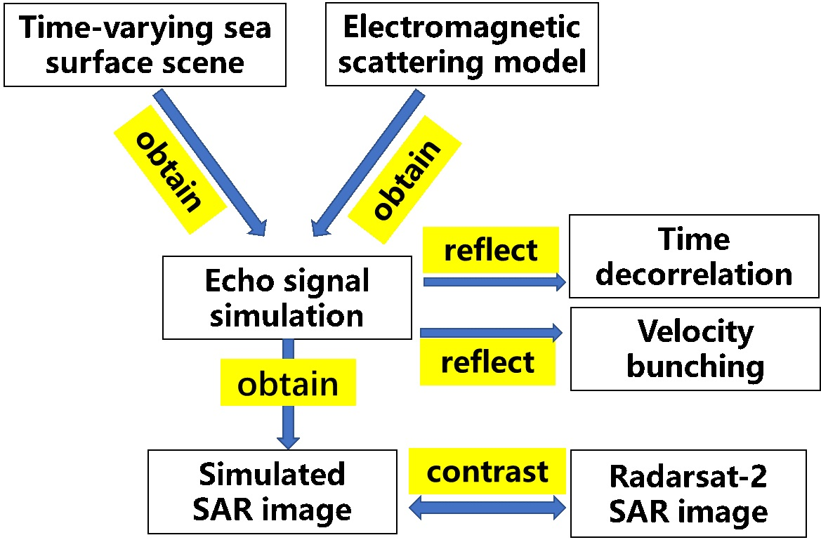
2. Modeling of Sea Surface Scene and Electromagnetic Scattering

A geometric relationship between SAR and the sea surface scene is as shown in Figure 1. In this paper, a zero squint angle and side-looking stripmap SAR system is adopted; its flight direction is along the azimuth direction (y-axis), the platform altitude is H (along the z-axis), and the flight velocity of the platform is V . The SAR transmits pulse signals continuously along the slant range direction; here, R C and θ represent the slant range and incident angle from SAR system to the center of the sea surface scene, respectively.

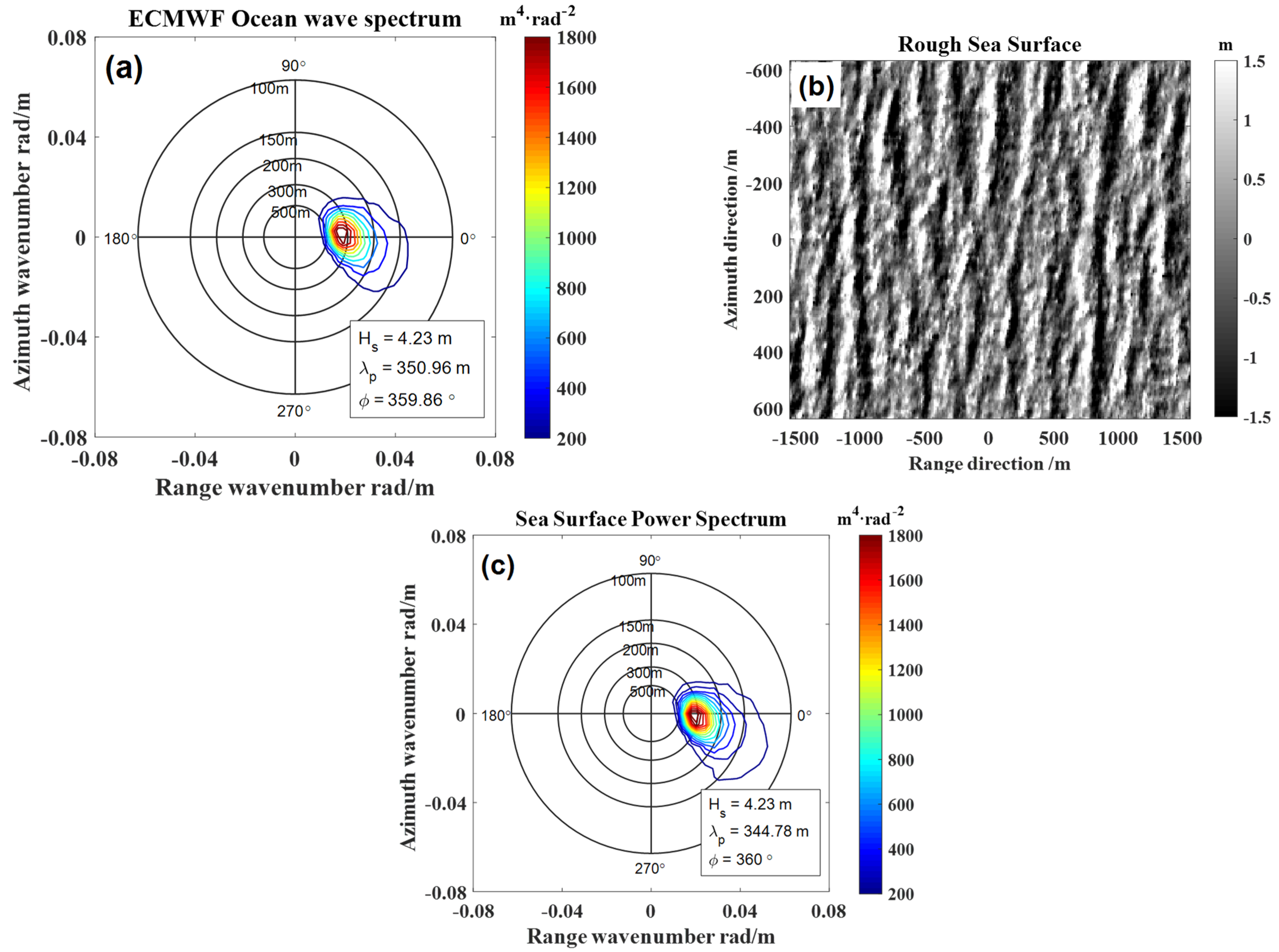
2.1. Modeling of Sea Surface Scene

In the process of SAR image simulation, the profile and the orbital velocity of the time-varying sea surface should be simulated first. In this work, the line filtering method, which has been widely used to simulate rough sea surface, is chosen to generate the two-dimensional sea surface. Based on this method, the time-varying sea surface profile, the slope along range direction, and the orbital velocity can be expressed as follows, according to [29]:
z ( x m , y n , t i ) = 1 L x L y m k = N x / 2 + 1 N x / 2 n k = N y / 2 + 1 N y / 2 F ( k m k , k n k ) exp [ i ( k m k x m + k n k y n ω m k , n k t i ) ] ,
s x ( x m , y n , t i ) = 1 L x L y m k = N x / 2 + 1 N x / 2 n k = N y / 2 + 1 N y / 2 i k m k F ( k m k , k n k ) exp [ i ( k m k x m + k n k y n ω m k , n k t i ) ] ,
v x ( x m , y n , t i ) = 1 L x L y m k = M / 2 + 1 M / 2 n k = N / 2 + 1 N / 2 ω m k n k k m k k F ( k m k , k n k ) exp [ i ( k m k x m + k n k y n ω m k n k t i ) ] ,
v y ( x m , y n , t i ) = 1 L x L y m k = M / 2 + 1 M / 2 n k = N / 2 + 1 N / 2 ω m k n k k n k k F ( k m k , k n k ) exp [ i ( k m k x m + k n k y n ω m k n k t i ) ] ,
v z ( x m , y n , t i ) = 1 L x L y m k = M / 2 + 1 M / 2 n k = N / 2 + 1 N / 2 i ω m k n k F ( k m k , k n k ) exp [ i ( k m k x m + k n k y n ω m k n k t i ) ] ,
where z and s x denote the profile and the slope of the sea surface, respectively, and v x , v y , and v z represent the velocity components of the orbital velocity along the x-axis, y-axis, and z-axis, respectively. m = 1 , 2 , , N x and n = 1 , 2 , , N y ; N x and N y are the discrete numbers of the surface along the range and azimuth directions, respectively; x m = m Δ x , y n = n Δ y , and Δ x and Δ y are the sampling intervals. t i is slow time. L x and L y denote the widths of the simulated sea surface; k m k = m k 2 π / L x and k n k = n k 2 π / L y represent the spatial wavenumber of sea waves along the range and azimuth directions, respectively. ω m k , n k = g k is the angular frequency with k = k m k 2 + k n k 2 . g is the gravitational acceleration, and F ( k m k , k n k ) denotes the Fourier coefficient of the rough sea surface, which can be expressed as
F ( k m k , k n k ) = 2 π [ L x L y W ( k m k , k n k ) ] 1 / 2 × { [ N ( 0 , 1 ) + i N ( 0 , 1 ) ] 2 , m k 0 , N x / 2   and   n k 0 , N y / 2 N ( 0 , 1 )              , others
where N ( 0 , 1 ) denotes random numbers that satisfy normal distribution and W ( k m k , k n k ) is the ocean wave spectrum in the Cartesian coordinate system. In this paper, wind waves and swells are both considered, and the ocean wave spectrum can be written as
W ( k m k , k n k ) = W w i n d ( k m k , k n k ) + W s w e l l ( k m k , k n k )
Using the following transformation relationship, the ocean wave spectrum within the Cartesian coordinate system is obtained as
W ( k m k , k n k ) = W ( k , φ ) k d k d φ d k m k d k n k ,
where W ( k , φ ) = W ( k ) ϕ ( k , φ ) denotes ocean wave spectrum within the polar coordinate system, W ( k ) is the omnidirectional spectrum, ϕ ( k , φ ) = [ 1 + Δ ( k ) cos ( 2 φ ) ] / 2 π denotes the angular spreading function, and φ is the angle between the wave propagation direction and the wind direction. The Elfouhaily spectrum [30] is proposed based on experimental data and theoretical facts. This spectrum is a global spectrum which can be used to describe the gravity waves and the capillary waves. In this paper, the Elfouhaily spectrum is used to generate wind waves because it can describe the capillary wave more accurately, and it is obtained that
W w i n d ( k ) = k 4 ( B l + B h ) ,
where B l and B h represent the curvature spectrum and l and h indicate low and high frequencies, respectively. In general, the narrow Gaussian spectrum is chosen to describe the swells. The expression of the the narrow Gaussian spectrum can be expressed as
W s w e l l ( k ) = σ s w e l l 2 2 π δ k 2 exp [ ( k k s _ p ) 2 2 δ k 2 ]
where σ s w e l l is the root-mean-square height of the simulated swell, k s _ p denotes the wavenumber at the peak of the Gaussian spectrum, and the spectral width is represented by δ k .

2.2. Modeling of Electromagnetic Scattering

Traditional SAR systems usually work at moderate incident angles, and the backscattered echoes are dominated by the scattering fields from small-scale Bragg resonance water waves. Because the spatial scale of the resolution cell in SAR images is much larger than the wave length of the Bragg resonance water waves, the two-scale scattering model can be employed to analyze scattering properties from the sea surface. Based on the two-scale model, ocean waves can be divided into large-scale and the small-scale waves. The small-scale waves are not only tilted in accordance with the slope distribution of the large-scale waves but also affected by the hydrodynamic modulation of the large-scale waves. The tilt modulation of the large-scale waves changes the local incidence angle at each resolution cell. The hydrodynamic modulation would cause nonuniform distribution of the roughness of the small-scale waves. Considering the effects of the tilt and hydrodynamic modulations, the normalized radar cross section (NRCS) can be expressed as
σ H H / V V ( x m , y n , t i ) = σ H H / V V ( θ ) + σ H H / V V ( θ ) 1 L x L y m k = N x / 2 + 1 N x / 2 n k = N y / 2 + 1 N y / 2 H y F ( k m k , k n k ) exp [ i ( k m k x m + k n k y n ω m k , n k t i ) ] ,
where the local incidence angle θ θ s x and θ denotes the incidence angle. σ p p ( θ ) = a 0 p p ( θ , U 10 ) [ 1 + a 1 p p ( θ , U 10 ) cos ( ϕ ) + a 2 p p ( θ , U 10 ) cos ( 2 ϕ ) ] denotes the normalized radar cross section evaluated by the CSAR GMF [31], which can be used to evaluated the mean values of the HH- and VV-polarized NRCS from the sea surface. ϕ is the azimuth angle of wind direction, U 10 denotes the wind speed 10 m above the sea surface, pp stands for polarization, and the details of the coefficients a 0 p p , a 1 p p , and a 2 p p can be found in [31]. H y denotes the hydrodynamic modulation transfer function (MTF) [4]. Unfortunately, up to now, the hydrodynamic modulation transfer function (HMTF) H y is less well-known. Based on the weak hydrodynamic interaction theory, a theoretical value for H y was derived in papers [32,33]. However, it is questionable whether this theory yields a realistic value of H y because it does not include the wind-induced straining [2]. Since the hydrodynamic modulation function of small-scale ripples by nonlinear long waves is under investigation so far, the H y developed in [2] is employed in this paper:
H y = ω l j μ ω l 2 + μ 2 ω l | K l | ( K l K s ) [ 1 W s K l W s K s 1 2 K l K s | K s | 2 ] ,
where K l and K s denote the wave number of the large-scale and the small-scale waves, respectively. W s denotes the roughness spectrum of the small-scale waves which are not modulated by the large-scale waves, and μ is the relaxation rate and has to be determined by experiment. However, the relaxation rate is poorly known experimentally. Moreover, the values estimated by various investigators differ by almost one order of magnitude [34]. In the present work, the value of the relaxation rate for C-band microwaves is obtained by interpolating the values of μ corresponding to L-band and X-band microwaves. Here, we take the following values for μ as reference values: μ = 0.92 s 1 for wind speeds ≥ 7 m/s and μ = 0.13 s 1 for lower wind speeds.
If we suppose that the 2D small-scale waves can be described by a roughness spectrum with a | K | 4 dependence [2], the hydrodynamic modulation function H y takes a simple form:
H y = 4.5 | K l | ω l ω l j μ ω l 2 + μ 2

2.3. The Temporal Decorrelation Analysis

Within a SAR resolution cell, there are many statistically scattering elements. Speckle noise would appear in the SAR image due to the coherent superposition of the echoes from the scattering elements. If the scattering elements within a SAR resolution cell are assumed to be uncorrelated with each other, the complex scattering field from a resolution cell satisfies the circular Gaussian distribution and can be generated by random numbers, i.e.,
γ ( x m , y n , t i ) = N 1 [ 0 , σ H H / V V ( x m , y n , t i ) ] + i N 2 [ 0 , σ H H / V V ( x m , y n , t i ) ] 2
where N 1 [ 0 , σ H H / V V ( x m , y n , t i ) ] and N 2 [ 0 , σ H H / V V ( x m , y n , t i ) ] represent two independent Gaussian random numbers. The expectation and the variance of the Gaussian random numbers are 0 and σ H H ( x m , y n , t i ) , respectively.
In the SAR imaging process, the backscattered complex signals of different pulses would coherently superpose together within SAR integration time. The high resolution along the azimuth direction is attained only if the backscattered complex scattering field remains coherent. The random motions of the small-scale water waves result in the temporal decorrelation of the scattering fields within SAR integration time. In this paper, the influence of the temporal decorrelation between the fields of the different pulses is considered by adding a random phase difference, which approximately satisfies the Gaussian distribution. Thus, the relationship between the complex scattering field at time t i and at t i 1 can be written as
γ ( x m , y n , t i ) = γ ( x m , y n , t i 1 ) exp ( i ψ ) ,
where the phase difference ψ can be approximately evaluated by
p ( ψ ) = 1 2 π σ ψ exp [ ( ψ ψ m ) 2 2 σ ψ 2 ]
Here, ψ m = 0 denotes the expectation of phase difference ψ , and σ ψ is the standard deviation of phase difference. Using σ v r denotes the standard deviation of the radial velocity of the small-scale waves within a resolution cell, and the relation between σ ψ and σ v r can be expressed as
σ ψ = 2 k e σ v r Δ t ,
where k e is the wavenumber of the incident electromagnetic wave. The time lag Δ t = t i t i 1 denotes the pulse repetition time. The standard deviation of the radial velocity, i.e., σ v r can be evaluated by
σ v r = v r 2 _ _ v ¯ r 2 = 1 2 0 + 0 + | T k v | 2 ( 1 C 2 ) W ( k m k , k n k ) d k m k d k n k
where C = sin ( k m k ρ r / 2 ) sin ( k n k ρ a / 2 ) ( k m k ρ r / 2 ) ( k n k ρ a / 2 ) , ρ r and ρ a are the range resolution and the azimuth resolution, respectively. Here, T k v = ω ( sin θ k m k k + i cos θ ) is the radial velocity transfer function.

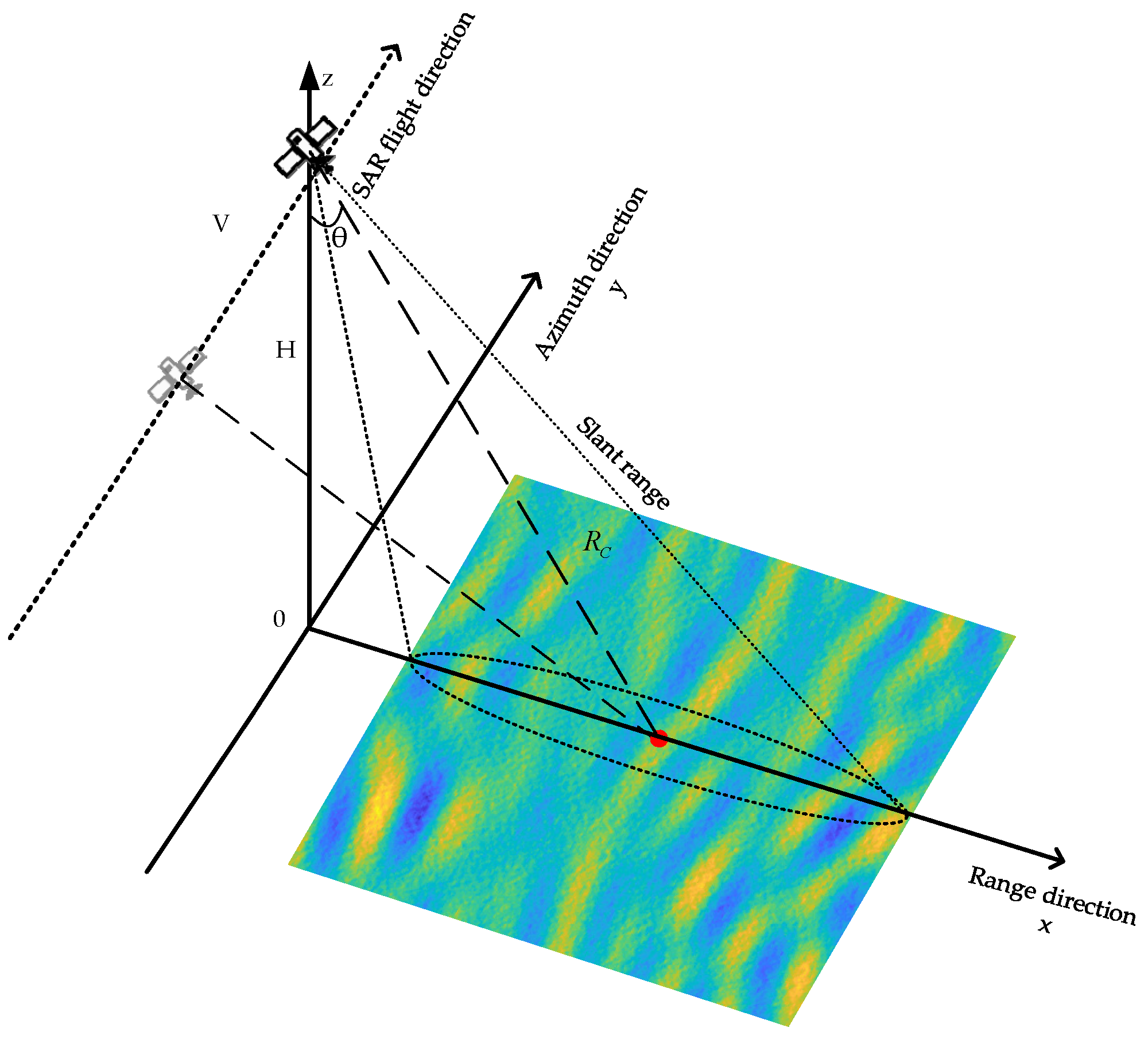
3. SAR Imaging Processing of Time-Varying Sea Surface

The geometry of the SAR sea wave imaging system is shown in Figure 1. The SAR system transmits linear frequency modulation (LFM) signals to the sea surface and receives echo signals from the sea surface. In order to obtain the SAR image of the observed sea surface scene, the pulse compression technique of the received echo signal is required. The RD algorithm is used in this paper because it is the most widely used algorithm for the spaceborne high-resolution SAR image processing. The time-varying sea surface SAR echo signal can be expressed as follows according to [35]:
s 0 ( τ , t i ) = m = M / 2 + 1 M / 2 n = N / 2 + 1 N / 2 γ ( x m , y n , t i ) rect [ τ 2 R ( x m , y n , t i ) / c T r ] exp [ ( t i t c ) 2 T a 2 ] exp [ j 4 π f 0 R ( x m , y n , t i ) c ] exp { j π K r [ τ 2 R ( x m , y n , t i ) c ] 2 }
where τ denotes fast time variable of SAR raw echo signal, and t c is the Doppler centroid time. rect ( ) is the range signal envelope, which is an approximately rectangular window, and the azimuth antenna pattern function is assumed to be a Gaussian function. f 0 is the radar carrier frequency, K r is the range frequency modulation (FM) rate, c is the speed of light, and R ( x m , y n , t i ) is the instantaneous slant range from the SAR to the sea surface.
SAR uses the Doppler history of signals to achieve fine azimuth resolution. Based on the “stop-and-go” assumption, we can assume that ocean waves are stationary at time t i . Thus, the slant range in the (19) can be expressed as
R ( x m , y n , t i ) = [ R 0 ( x m , y n ) v r ( x m , y n , t i ) ( t i t c ) ] 2 + { [ V v y ( x m , y n , t i ) ] ( t i t c ) } 2 R 0 ( x m , y n ) v r ( x m , y n , t i ) ( t i t c ) + V 2 2 R 0 ( x m , y n ) ( t i t c ) 2
where R 0 ( x m , y n ) = ( H z ( x m , y n ) ) 2 + x m 2 is the closest slant range from the SAR to each stationary scattering facet of sea surface, V is the SAR platform velocity, v r ( x m , y n , t i ) = v x ( x m , y n , t i ) sin θ + v z ( x m , y n , t i ) cos θ denotes the instantaneous radial velocity, and v y ( x m , y n , t i ) is the azimuthal velocity of the surface scattering element on the large-scale waves. For ocean waves, v y ( x m , y n , t i ) V , and thus the influence of azimuthal velocity, can be neglected.
The echo signal in (19) is the SAR raw signal without focusing. The implementation process of the RD algorithm is as follows:
  • After the fast Fourier transform (FFT) along the range direction, the SAR raw echo signal in range frequency domain can be expressed as
    s 0 ( f τ , t i ) = m = M / 2 + 1 M / 2 n = N / 2 + 1 N / 2 γ ( x m , y n , t i ) rect [ f τ K r T r ] exp [ ( t i t c ) 2 T a 2 ] exp [ j 4 π ( f 0 + f τ ) R ( x m , y n , t i ) c ] exp { j π f τ 2 K r }
    The SAR raw echo signal is multiplied by the range-matched filter H r ( f τ ) in the range frequency domain to remove the second-order phase term of fast time τ . The range-matched filter is given by
    H r ( f τ ) = rect ( f τ | K r | T r ) exp ( + j π f τ 2 K r ) ,
    where T r is chirp pulse duration, f τ is the range frequency, rect ( ) denotes the rectangular window, and K r denotes the range FM rate. The echo signal after the range compression is expressed as
    s r c ( τ , t i ) = IFFT r { S 0 ( f τ , t i ) H r ( f τ ) }
  • The change of the instantaneous slant range will result in range cell migration, which needs to be corrected. Range cell migration correction is performed after range compression and before azimuth compression. The echo signal and the slant range formula in the range-Doppler (RD) domain are obtained by azimuthal FFT and are given by
    S r c ( τ , f t i ) = FFT a [ s r c ( τ , t i ) ]
    and
    R ( x m , y n , f t i ) = FFT a [ R ( x m , y n , t i ) ] = R 0 ( x m , y n ) + Δ R ( x m , y n , f t i ) ,
    where Δ R ( x m , y n , f t i ) is the range migration in the range-Doppler domain. The echo signal is discrete sampling, so the corrected discretized echo signal can be expressed as
    S r c m c ( p , q ) = S r c ( p , q + 2 Δ R ( p , q ) F r / c )
    where p and q are the discretized range time series and the discretized azimuth frequency series, respectively, Δ R ( p , q ) is the discretized range migration, and F r is the range sampling rate. The correcting value 2 Δ R ( p , q ) F r / c may be non-integer, so the sin c interpolation operation can be used for the range cell migration correction (RCMC).
  • An azimuth matched filter H a z ( f t i ) in the range-Doppler domain is used to achieve azimuth compression and can be given by
    H a z ( f t i ) = exp ( j π R λ 2 V 2 f t i 2 )
    The 2D time domain complex amplitude of compressed signal s a c ( τ , t i ) is obtained after inverse fast Fourier transform (IFFT) along the azimuth direction.
    s a c ( τ , t i ) = IFFT a { S r c m c ( τ , f t i ) H ( f t i ) }
The above is the process for the actual imaging of time-varying sea scenes.
To clearly demonstrate the effects of ocean wave radial velocity and acceleration on SAR imaging, under the assumption that the radial velocity and acceleration of the scattering surface facet can be replaced by their mean values, specific theoretical formulations for azimuthal compression are given below. The size of the scattering facet equals the size of the SAR resolution cell. The mean radial velocity and acceleration in the SAR integral time are represented by v r ( x m , y n ) ¯ and a r ( x m , y n ) ¯ , respectively. Thus, (20) can be approximated as
R ( x m , y n , t i ) R 0 ( x m , y n ) v r ( x m , y n ) ¯ ( t i t c ) + V 2 2 R 0 ( x m , y n ) ( t i t c ) 2 a r ( x m , y n ) ¯ 2 ( t i t c ) 2 ,
For ocean waves, the effect of the radial velocity and acceleration on SAR imaging along the range direction is relatively small and can be neglected. In this paper, we mainly analyze the effects on the azimuthal imaging. Therefore, after range compression and RCMC, the expression of the echo signal is given directly by
s r c m c ( τ , t i ) = m = M / 2 + 1 M / 2 n = N / 2 + 1 N / 2 γ ( x m , y n , t i ) | K r | T r sin c r [ | K r | T r ( τ 2 R ( x m , y n ) / c ) ]   exp [ ( t i t c ) 2 T a 2 ] exp { j 4 π R ( x m , y n , t i ) λ }
The range signal envelope has been focused into the sinc function, and the range resolution is given by
ρ r = c 2 B = c 2 | K r | T r ,
The azimuth matched filter in the slow time domain is
h ( t i ) = exp { + j π 2 V 2 R λ t i 2 }
The azimuthal compression is achieved by convolution with the time domain matched filter as follows
s a c ( τ , t i ) = s r c m c ( τ , t i ) h ( t i ) ,
The ensemble-averaged SAR image intensity can be calculated by substituting (29), (30), and (32) into (33) [1,3], i.e.,
I a c ( τ , t i ) = π 2 | K r | 2 T r 2 T a 2 m = M / 2 + 1 M / 2 n = N / 2 + 1 N / 2 | γ ( x m , y n ) | 2 ¯   sin c 2 r [ | K r | T r ( τ 2 R ( x m , y n , t i ) / c ) ]   × ρ a ρ a ( x m , y n ) exp [ π 2 V 2 ρ a 2 ( x m , y n ) ( t i t c R 0 ( x m , y n ) v r ( x m , y n ) _ _ _ _ _ _ _ _ _ _ _ _ _ V 2 ) 2 ]
where
ρ a = λ R 2 V T a
is the resolution for the stationary sea surface. For time-varying sea surfaces, the degraded azimuthal resolution is
ρ a = [ ρ a 2 + ( π 2 R V a r _ _ T a ) 2 + ( ρ a T a t s ) 2 ] 1 / 2
Since radial average acceleration a r ( x m , y n ) ¯ causes the mismatch in the azimuthal matched filtering, there are residual quadratic phases, which can lead to the degradation of the azimuthal resolution of the integrated intensity image. The time-varying complex scattering field γ ( x m , y n , t i ) can decrease scene coherence time, resulting in temporal decorrelation and thus also leading to azimuthal resolution degradation. t s represents the sea surface scene coherence time, which is mainly determined by the spread of radial velocity within a resolution cell, and it can be given by
t s = λ 2 π 2 σ v r
According to (34), one can find that the azimuthal imaging position is at the moment t i = t c when the sea surface is stationary. However, the imaging moment is t i = t c + R 0 ( x m , y n ) v r ( x m , y n ) _ _ _ _ _ _ _ _ _ _ _ _ _ V 2 for time-varying sea surfaces. Therefore, the radial velocity of the surface scattering element would induce a displacement along the azimuth direction in the SAR image. This azimuth displacement is given by
ζ = β v r ( x m , y n ) _ _ _ _ _ _ _ _ _ _ _ _ _ = R 0 V v r ( x m , y n ) _ _ _ _ _ _ _ _ _ _ _ _ _ ,
where β is the range-to-velocity ratio of the SAR platform. Just because of this azimuth displacement, the periodic orbital motion of the larger-scale waves will produce an apparent increase and decrease in the density of scatters, known as the velocity bunching effect (VB), thereby making azimuth-traveling long waves detectable on the SAR image plane, albeit shifted from their true position. However, as the radial velocity components of the large-scale waves increase, more random azimuth displacements would appear. If the minimal displacement is less than a wavelength of the azimuth-traveling large-scale water wave, the azimuth-traveling large-scale water waves will be linearly mapped in the SAR imagery. Otherwise, if the azimuthal displacement is larger than the wavelength of the azimuth-traveling large-scale water wave, the mapping of the azimuth-traveling large-scale water waves on SAR imagery will be nonlinear and distorted [5]. According to the above analysis, the VB effect on SAR images depends on the SAR system and ocean wave parameters. The VB effect makes it difficult to acquire ocean wave information from SAR images. Therefore, the subsequent simulation of SAR data with different parameters in this paper aims to analyze the effect of velocity bunching on SAR imaging of time-varying sea surfaces.

4. Verification of Simulation Method

To prove the availability of the SAR imaging simulation method, in this section, we contrasted SAR simulation data with actual SAR data in three aspects: the SAR image patterns feature, the SAR image spectrum feature, and the SAR image intensity distribution feature.

4.1. The Actual SAR Images and the Marine Environment Information

Nine quad-polarization RADARSAT-2 SAR images with clear swell patterns are presented for comparison with the simulated SAR images. The detailed information of the RADARSAT-2 SAR images is shown in Table 1. The parameters of the quad-polarization RADARSAT-2 SAR is shown in Table 2. In our simulations, the swells are simulated by (1)–(5) based on the reanalysis wave spectra of the European Centre for Medium-Range Weather Forecasts (ECMWF). Because velocity bunching has less influence on the patterns of the swells, especially when swells propagate along the SAR range direction, the patterns of the swells in the actual SAR images have good consistency with the patterns of the swells’ profiles. Therefore, in order to make the swells simulated by Equations (1)–(5) more consistent with the swells at the imaging time of the actual SAR images, the random phase of the Fourier coefficient F ( k m k , k n k ) of the swell profile in Equations (1)–(5) is replaced by the phase of the Fourier coefficient of the actual swell SAR image. On the other hand, the wind waves are simulated based on the Elfouhaily spectrum, and the wind speed and wind direction used in the Elfouhaily spectrum were the in-situ buoys of the National Data Buoy Center (NDBC). The significant wave height (SWH, H s ), the wavelength ( λ P ), and the propagation direction ( ϕ ) of the dominant waves of the reanalysis wave spectra and the wind information are listed in Table 1.

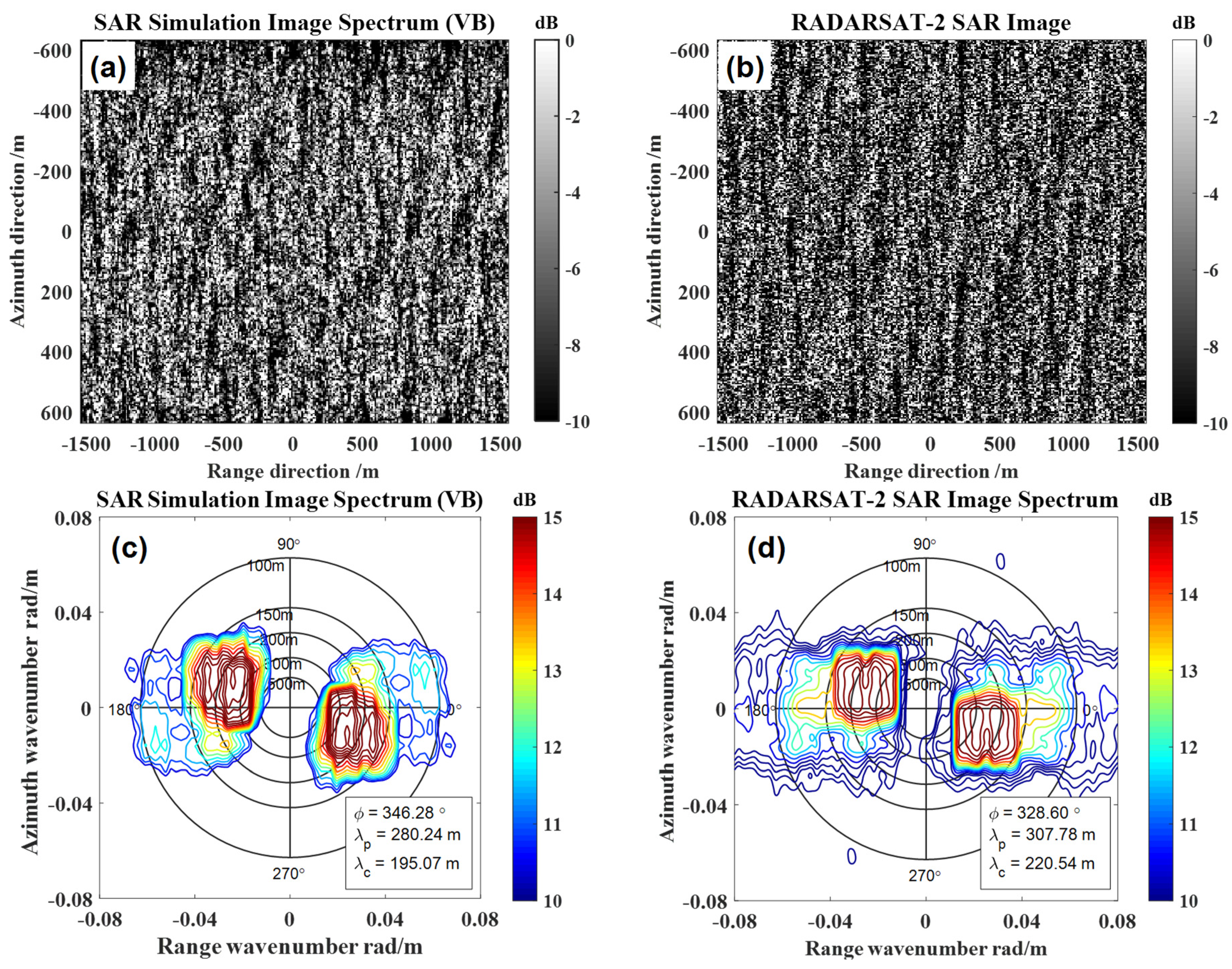
4.2. Contrast Experiment 1 with the Center Incidence Angle 23.27°

The reanalysis ocean wave spectrum corresponding to SAR ID 1 and the reconstructed sea surface are shown in Figure 2a,b, respectively. To verify the reliability of the reconstructed sea surface, the spectrum of the reconstructed sea surface in Figure 2b is also shown in Figure 2c. From the comparison between Figure 2a,c, it is found that that the spectrum of the reconstructed sea surface is very consistent with the input spectrum, i.e., the reanalysis ocean wave spectrum. This result proves the reliability of the reconstruction method of the sea surface profile.
Based on the parameters of the sea environment in Table 1 and the parameters of the quad-polarization RADARSAT-2 SAR in Table 2, the simulated SAR image corresponding to SAR ID 1 with the center incidence angle 23.27° is compared with the actual SAR image in Figure 3. In Figure 3, the simulated SAR image is compared with the actual SAR image in three aspects: image patterns, image power spectrum, and statistical distribution function of SAR speckle noise. Firstly, the simulated HH-polarized SAR NRCS images are shown in Figure 3a,b, respectively. Comparing the patterns in Figure 3a with those in the actual SAR image (i.e., Figure 3b), we can find that the textural features in the actual image have been successfully simulated by the simulation method proposed in this paper. In order to further quantitatively compare the consistency of the texture features in the simulated SAR image with those in the actual SAR image, the power spectra of the simulated and the actual HH-polarized SAR NRCS images are also presented in Figure 3c,d, respectively. In order to show the spectra more clearly, we take the logarithm of the power spectra intensities in the following. One can find that the spectral density of the simulated SAR image is in good agreement with that of the actual image. Speckle noise is another intrinsic feature of SAR image. In Figure 3e, the statistical probability density distribution of the SAR image intensity based on the simulated SAR data is also compared with that obtained by the actual SAR image. Just as expected, the two probability density distribution curves in Figure 3e agree well with each other.

4.3. Contrast Experiment 2 with the Center Incidence Angle 33.24°

The second contrast experiment is carried out in Figure 4. On the basis of the parameters of the sea environment and the RADARSAT-2 SAR system, the simulated SAR image corresponding to SAR ID 2 with the center incidence angle 32.24° is compared with the actual SAR image. From the comparison between the simulated and the actual SAR images in three aspects, we can find that the image patterns, the image spectrum, and the distribution function of speckle noise of the simulated SAR image are all consistent with those of the actual SAR image.

4.4. Contrast Experiment 3 with the Center Incidence Angle 39.96°

The third contrast experiment is carried out in Figure 5. On the basis of the parameters of the sea environment and the RADARSAT-2 SAR system, the simulated SAR image corresponding to SAR ID 3 with the center incidence angle 39.96° is compared with the actual SAR image. From the comparison between the simulated and the actual SAR images in three aspects, we can find that the image patterns, the image spectrum, and the distribution function of speckle noise of the simulated SAR image are all consistent with those of the actual SAR image.
To further analyze the validity of the SAR image simulation method, comparisons of the simulated SAR images (corresponding to the nine SAR images listed in Table 1) and the actual SAR images for the maximum spectral density, as well as the wavelength and propagation direction of the dominant wave, are presented in Figure 6. Figure 6a shows the comparison between the maximum values of the simulated and the actual SAR image spectra. The results show that the correlation coefficient, the mean-square error (RMSE), and the bias of the maximum spectral density are 0.78, 2.27 dB, and −1.41 dB, respectively. The wavelength and propagation direction of the dominant wave are compared in Figure 6b,c. It can be seen that the wavelengths and propagation directions of the dominant waves obtained from the simulated SAR images are very consistent with those obtained from the actual SAR images, and the correlation coefficients of these two parameters reach 0.97 and 0.95, respectively. The azimuthal cut-off wavelength is also consistent in Figure 6d. From the results in Figure 3, Figure 4, Figure 5 and Figure 6, however, we can find that there are still some differences between the simulated and the actual SAR images. These differences may be caused by the inconsistencies between forecast sea states and the real sea states at the actual SAR imaging times. However, overall, the comparisons between the simulated SAR image and the actual SAR image from Figure 3, Figure 4, Figure 5 and Figure 6 illuminate that SAR images can be well-simulated by the simulation method proposed in this work.

5. Discussion of Simulation Results

Under the premise that the radar spatial resolution is determined, SAR images of ocean waves would be still affected by many factors, such as platform altitude and velocity, radar frequency, radar incidence angle, wind speed and direction, the propagation direction of the swell, and so on. Among these factors, the influences of the velocity bunching effect, wind speed and direction, and the propagation direction of the swell are more significant. Therefore, in the following, the influences of these three main factors on SAR images of ocean waves will be discussed in detail.

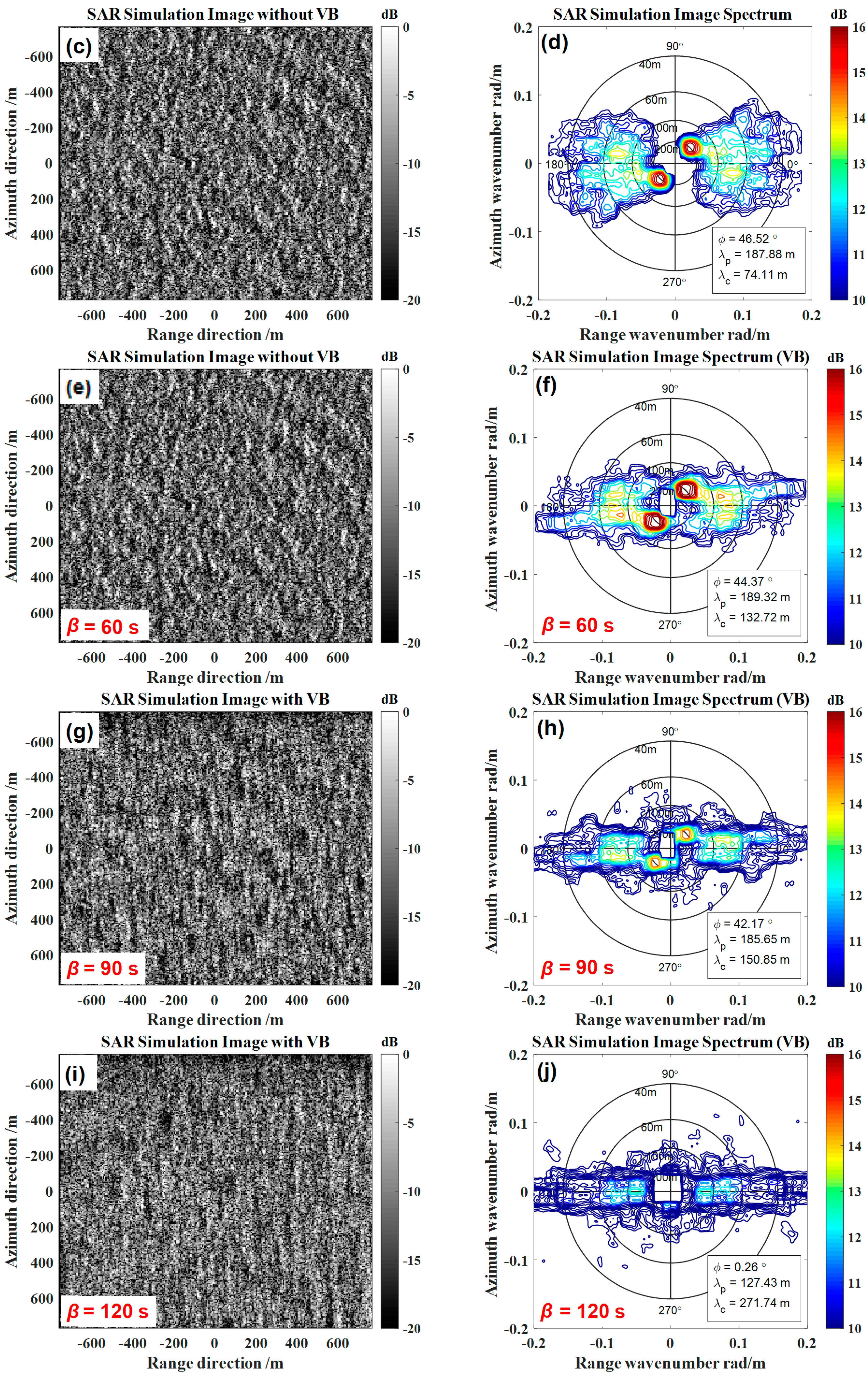
5.1. The Influence of the Velocity Bunching Effect

The influence of the VB effect on SAR images of ocean waves is closely related to the range-to-velocity ratio β (the ratio of slant range to platform velocity). With the value of β increasing, the influence of the VB effect becomes more significant. The simulated SAR images with different β are shown in Figure 7. The parameters of the radar system and the marine environment used in the simulation are given in Table 3. The simulated sea surface profile and the corresponding spectrum are shown in Figure 7a,b. The swell and wind waves can be clearly observed in the figures. The simulated HH-polarized SAR images for β = 60 s ( v r = 0 m / s ), β = 60 s, β = 90 s, and β = 120 s are shown in Figure 7c,e,g,i, respectively, and the corresponding SAR image spectra are presented in Figure 7d,f,h,j. As shown in Figure 7c, if the VB effect is not considered in the SAR image simulation procress, the textures in the simulated SAR image are consistent with those in the sea surface profile image. From the SAR image spectrum in Figure 7d, it is found that the spectral peaks corresponding to the wind waves and the swell in Figure 7b can be clearly observed. However, as shown in Figure 7e–j, with the increase in the range-to-velocity ratio, the influence of the VB effect becomes more obvious. The comparison between Figure 7c,e illuminates that the textures of large-scale waves on the simulated SAR image become clearer when β = 60 s and the VB effect is considered. However, the wind waves with short wavelengths are fuzzed by the VB effect, and the wind wave spectrum in Figure 7f has also been distorted. As the value of the parameter β continues to increase, the influence of the VB effect becomes more severe so that the textures of the large-scale waves become fuzzy. When β = 120 s, as shown in Figure 7i,j, the large-scale swell has been seriously distorted in SAR imagery, and the propogation direction of the swell is deflected to the SAR range direction. In this case, the serious velocity bunching effect makes it difficult to acquire accurate ocean wave information from the SAR image. From the SAR image spectra in Figure 7, the azimuthal cut-off in the SAR image spectrum due to the azimuth displacement and smear induced by the VB effect can be clearly seen. The azimuthal cut-off wavelength ( λ c ) increases with the increase in β, as shown in the Figure 7. This indicates that the larger the β value, the less able the SAR is to image the water waves that propagate along the azimuth direction. When large-scale swells are severely damaged (β = 120 s), the spectral peak wavelength ( λ P ) gets shorter. Besides, when the VB effect is considered, the spectral peaks ( ϕ ) of the SAR image rotate to the range direction as the value of β increases.

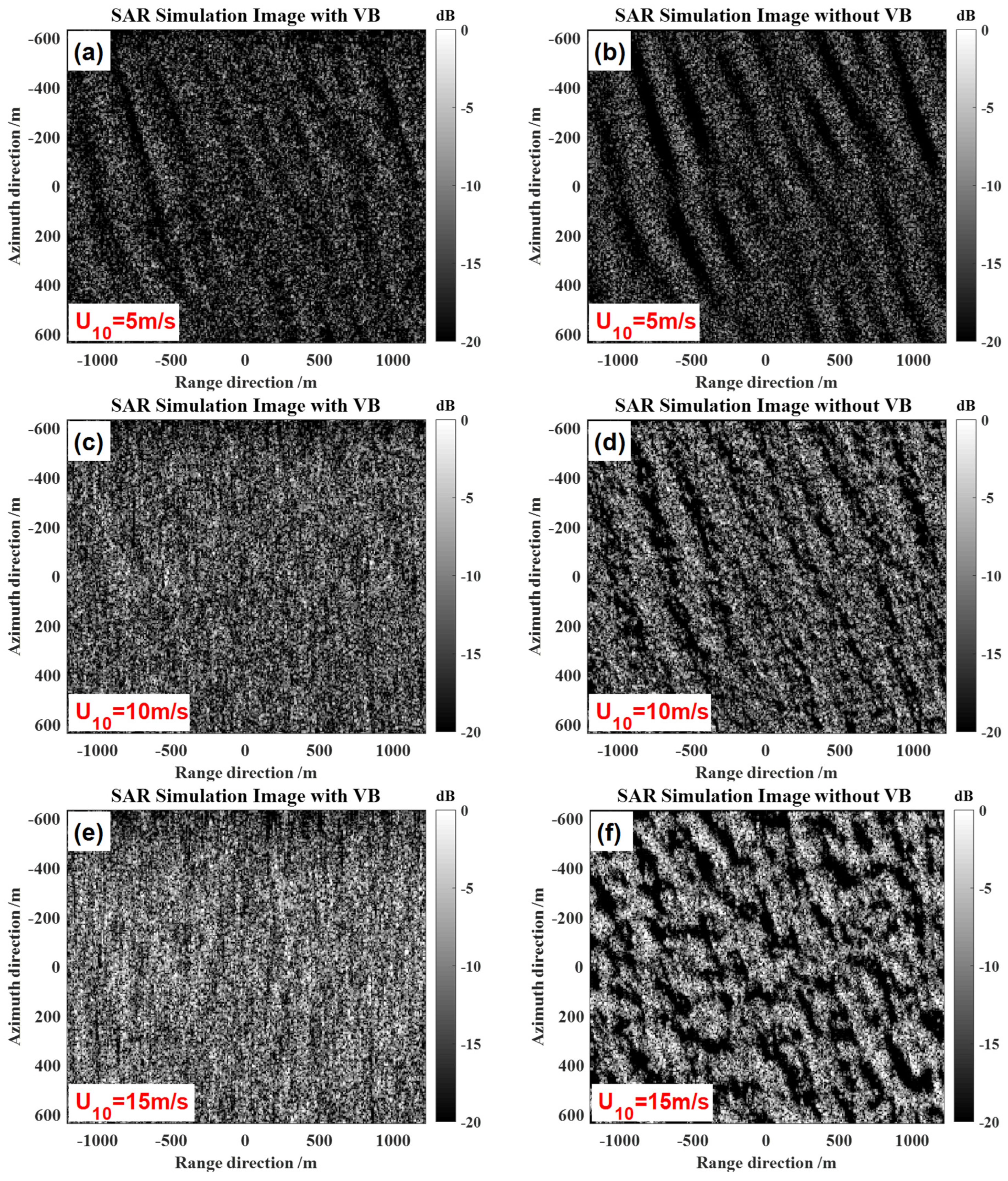
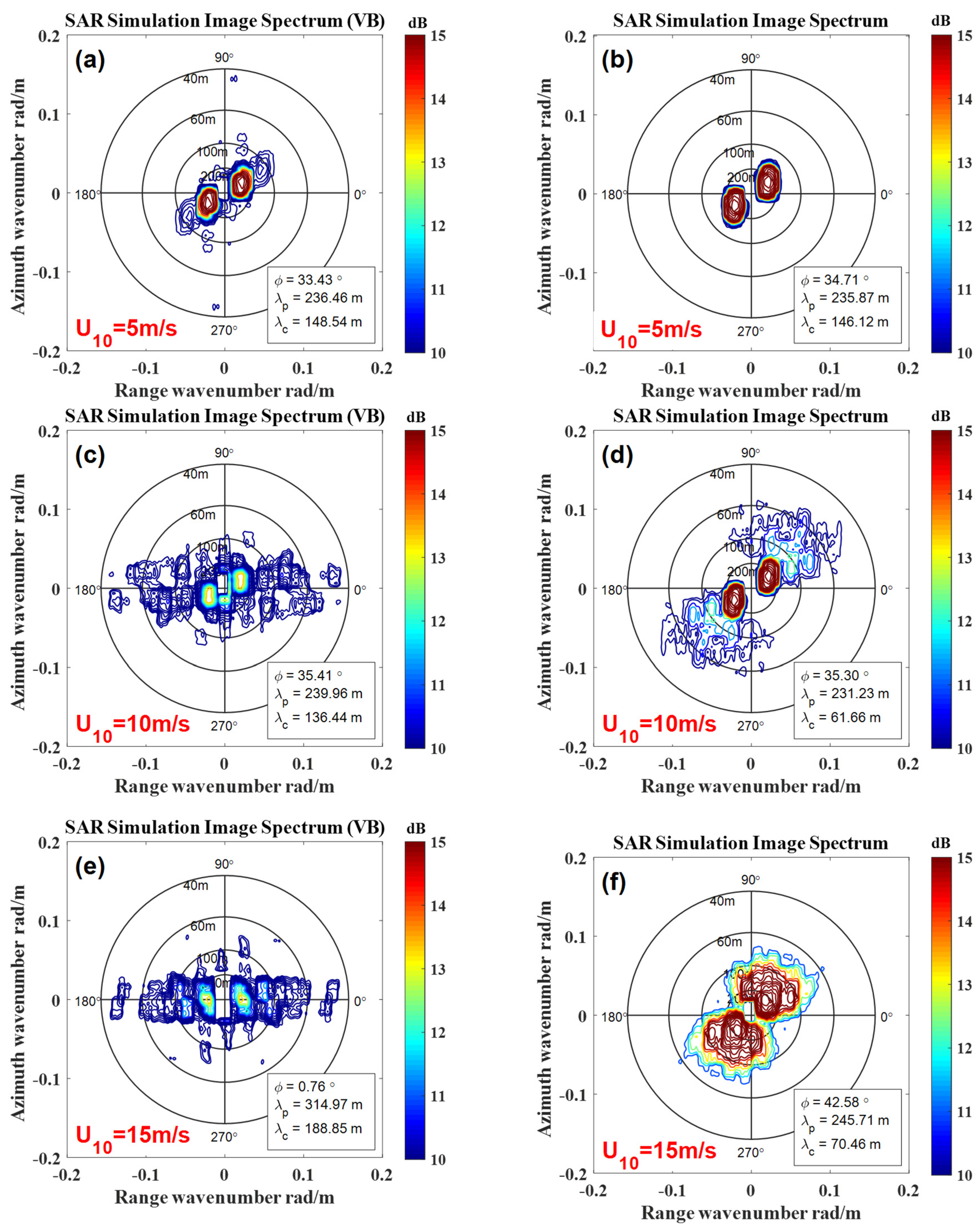
5.2. The Influence of Wind Speed

We discussed the influence of wind field because wind waves are directly determined by wind speed and wind direction. For different wind speeds and wind directions, the sea surface roughness and the orbital velocity of the wind waves would be significantly different. Then, wind speed and wind direction would induce remarkable influence on the SAR image. Figure 8 and Figure 9 show the influence of different wind speeds on SAR images and the corresponding SAR image spectra. The parameters used in the simulations are given in Table 4. Firstly, the comparisons of the simulated SAR images with and without the VB effect are shown in Figure 8. When the wind speed is 5 m/s, the radial velocity of the water waves is small, so the influence of the VB due to wind waves on the texture of the swell is not very significant. From the corresponding SAR image spectra shown in Figure 9a,b, the shapes of the spectral peaks of the SAR image spectra with and without considering the influence of VB effect are consistent with each other except for some differences in the spectral density. However, with the increase in wind speed, the influence of the wind waves on the texture of the swell becomes more obvious. Comparing Figure 8c,d, we can find that when the wind speed increases to 10 m/s, the textures of the swell in Figure 8c have been seriously smeared by the VB effect due to the orbital velocity of the wind waves. For this case, although the position of the spectral peak in Figure 9c is the same as in Figure 9d, the shape and the spectral density of the spectral peak have been changed significantly. Additionally, the spectral density of the SAR image spectrum with the VB effect is obviously lower than that without the VB effect. If the wind speed increases to 15 m/s, as shown in Figure 8e, the VB effect has made the textures of the swell completely invisible in the SAR image, only some stretched vertical stripes along the azimuth direction. From the corresponding SAR image spectrum shown in Figure 9e, we also find that the spectral peak has been rotated to the range direction. In addition, the azimuthal cut-off effect is more serious. From Figure 8 and Figure 9, we can find that if the influence of the VB effect has been considered, the information of the wind waves cannot be extracted from the simulated SAR images when wind direction is 60°.

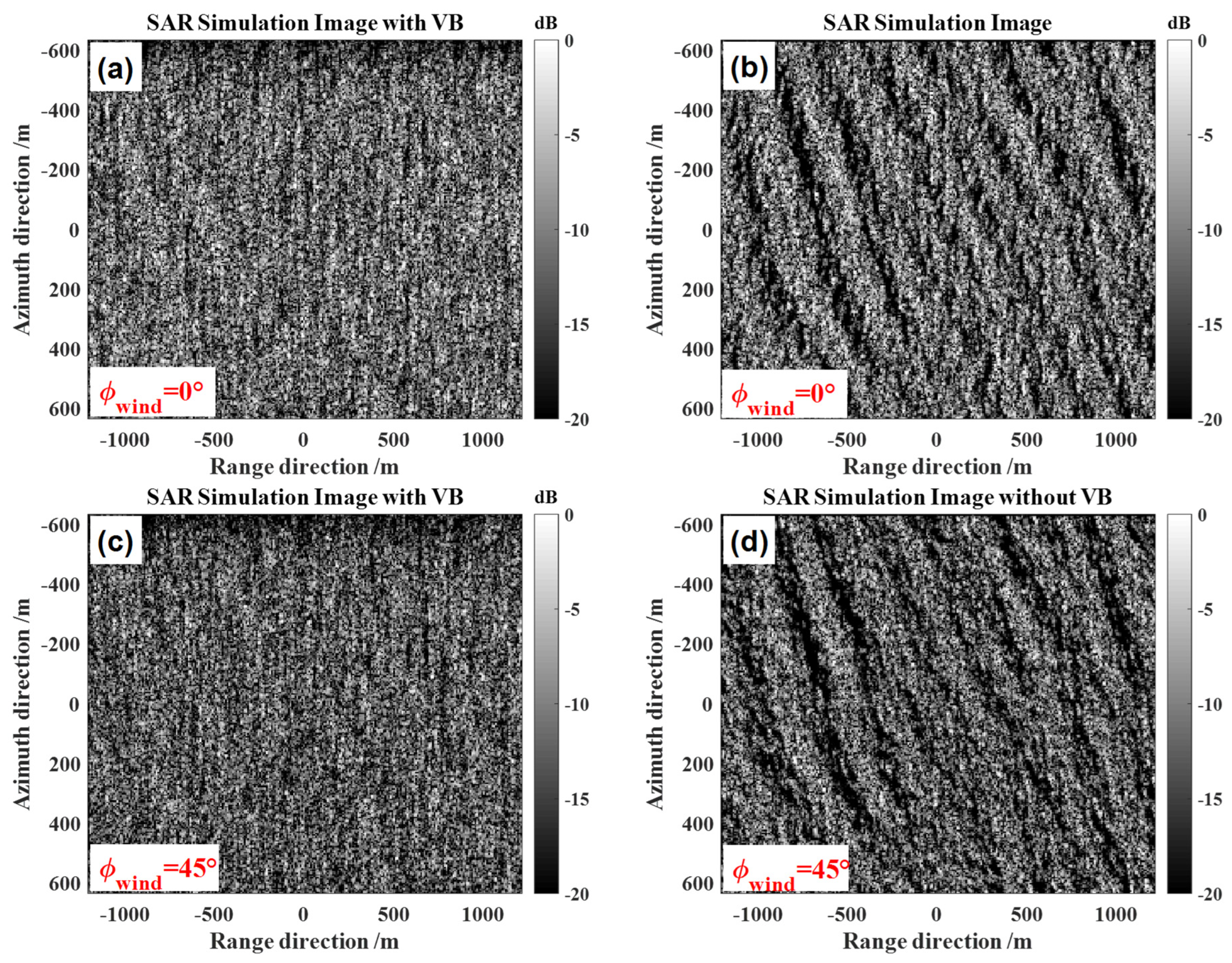
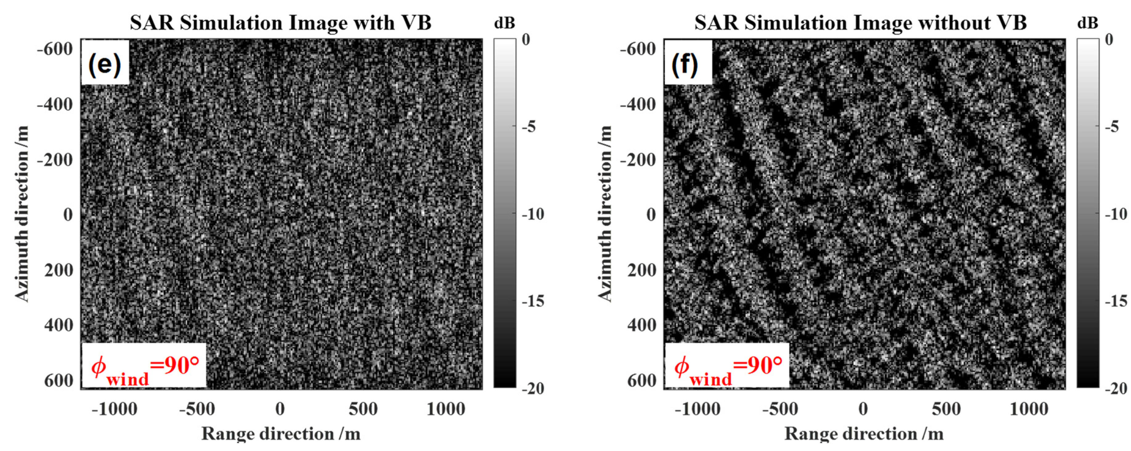
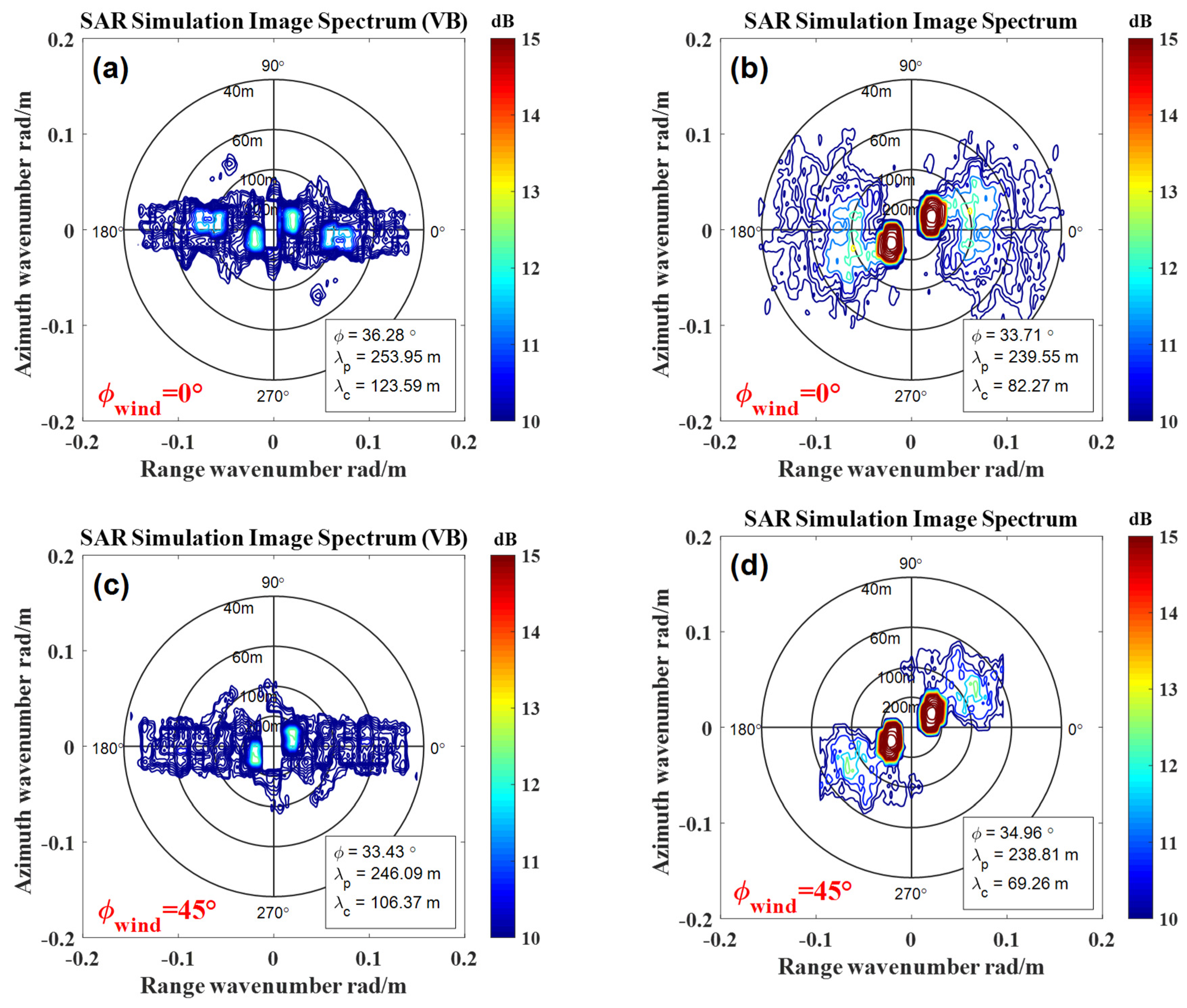
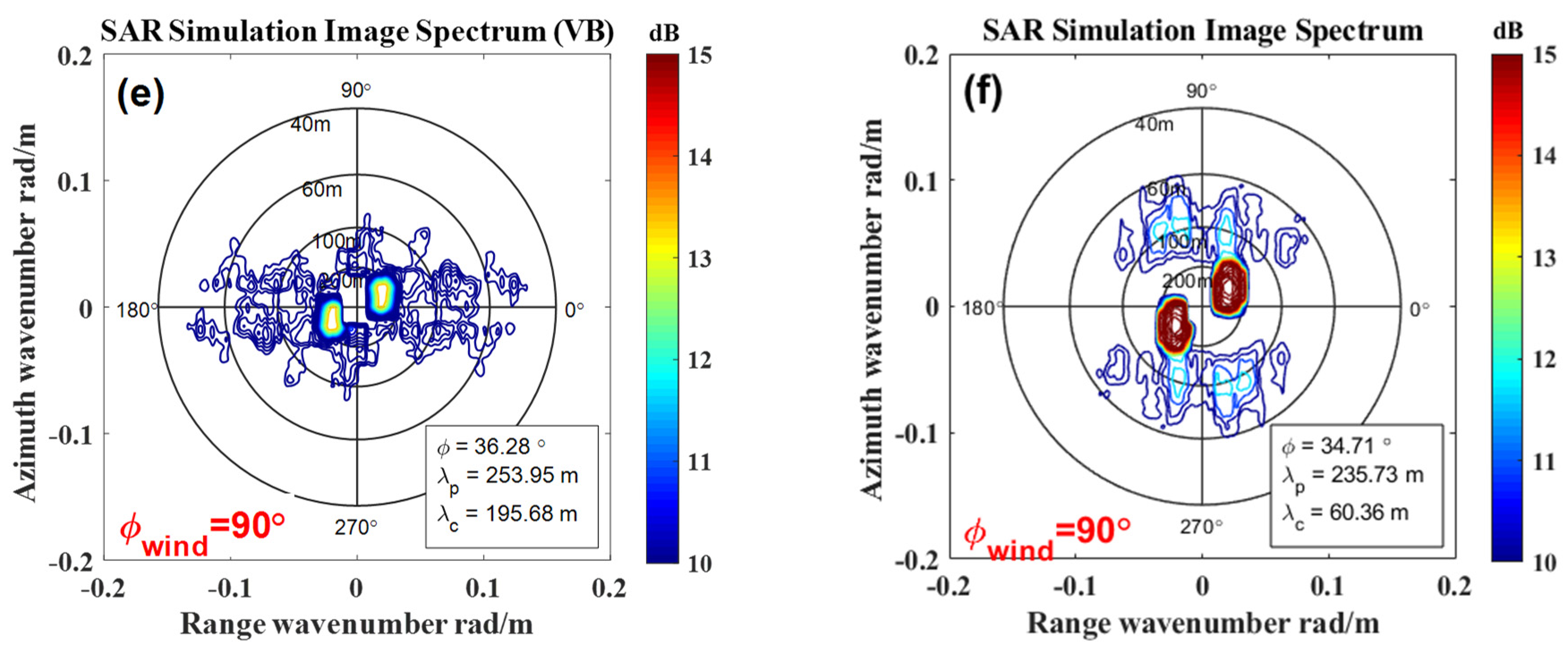
5.3. The Influence of Wind Direction

For wind waves, the direction of the dominant wave is along the wind direction. Table 5 shows the simulation parameters when the wind direction is 0°, 45°, and 90°. The input parameters of the radar are the same as in Table 4. Figure 10 and Figure 11 indicate the influence of different wind directions on SAR images and corresponding SAR image spectra. Figure 10a,c,e show the SAR images considering the VB effect when the wind direction is 0°, 45°, and 90°, respectively. Figure 10a illustrates that the VB effect also affects SAR imaging for wind waves propagating along the range direction, resulting in azimuth displacement of wind waves. The azimuthal cut-off effect can also occur for wind waves traveling along the range direction, as shown in Figure 11a. Meanwhile, the azimuthal cut-off wavelength in the wind direction of 45° is slightly less than that in the wind direction of 0°. The reason for this is that the radial velocity is the largest for the wind wave traveling along the range direction, and the azimuthal displacement caused by the VB effect will have an impact on the SAR imaging of short-wavelength, irregular wind waves. When wind waves propagate along 45°, not only does the VB effect cause azimuth stretching, but the peak wave direction also appears to rotate toward the range direction on the SAR image and image spectrum, as shown in Figure 10c and Figure 11c. Figure 10e shows the blurred SAR image, which indicates that for wind waves propagating in the azimuthal direction with irregular waveforms and short wavelengths, velocity bunching will cause the strong nonlinear effect. Unlike Figure 11f, the clear azimuthal cut-off effect can be seen in Figure 11e. The azimuthal cut-off wavelength ( λ c ) is 195.68 m, indicating that the VB effect is most significant for ocean waves propagating in the azimuth direction. In addition, wind direction can affect the sharpness of the swell in the SAR images, as shown in Figure 10.

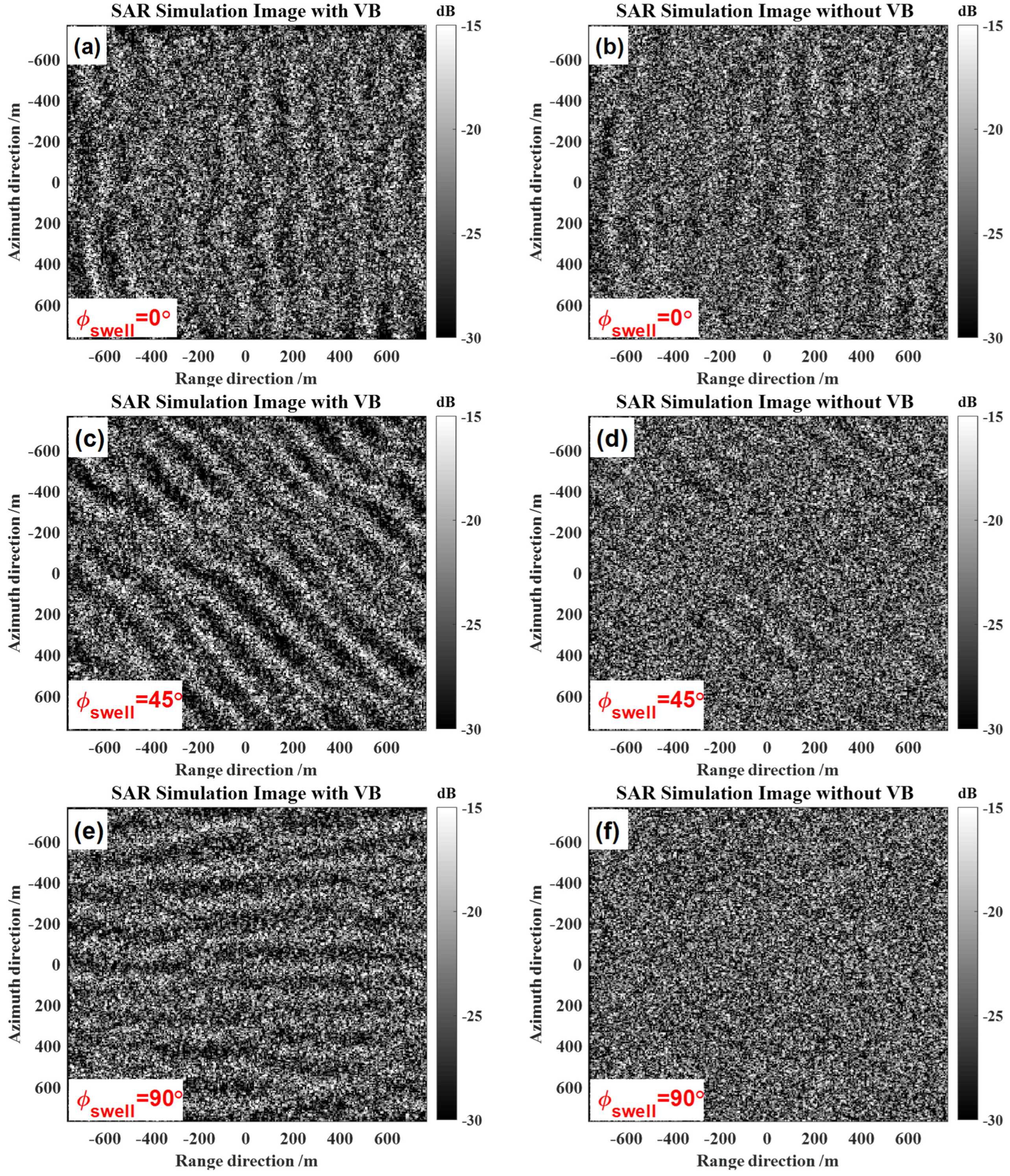
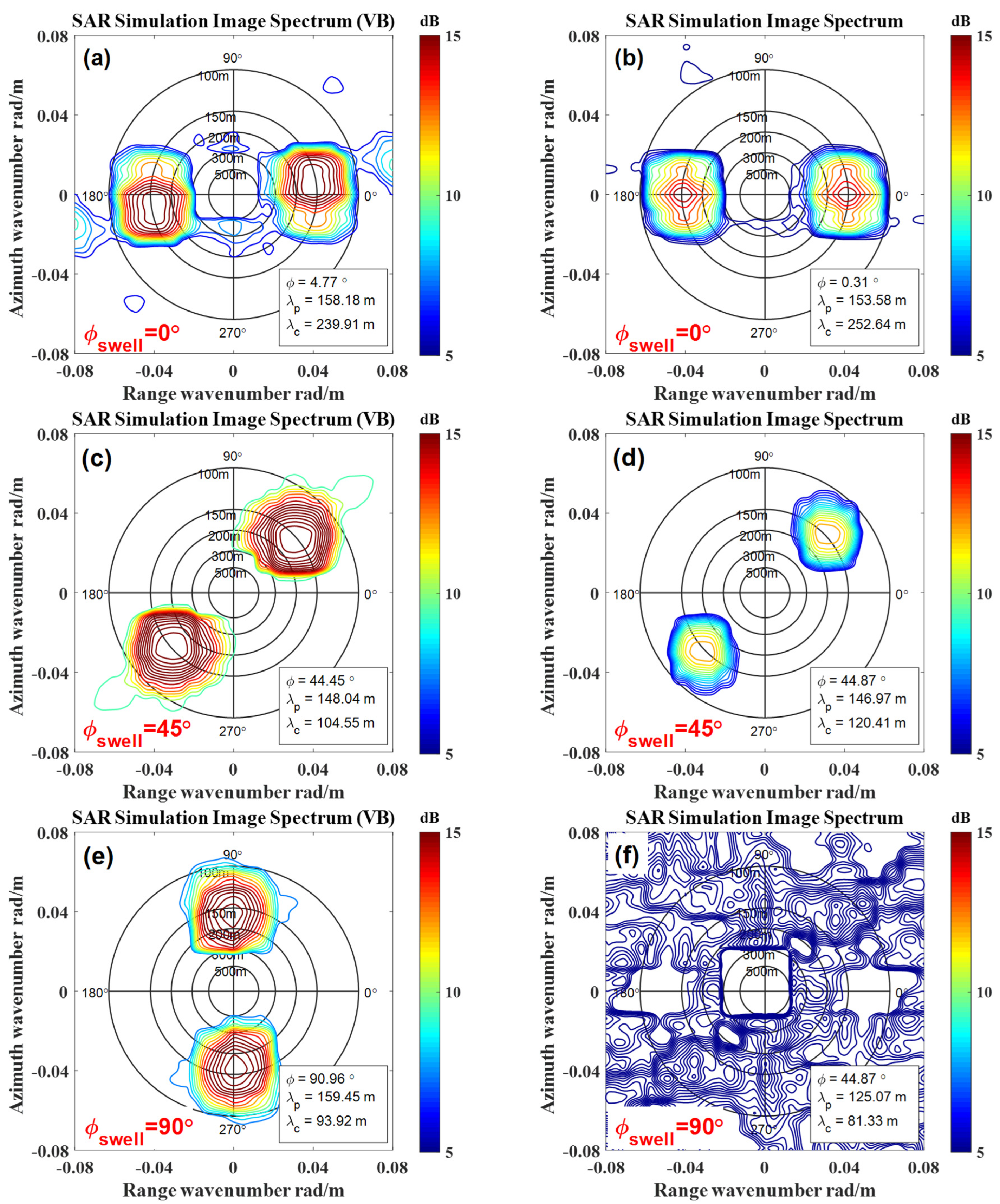
5.4. The Influence of Swell Direction

Table 6 shows the simulation parameters when the β value is 120 s, wind direction is 90°, wind speed is 5 m/s, swell directions are 0, 45, and 90°, and swell wavelength is 200 m. The other input parameters of radar are the same as in Table 3. Similarly, Figure 12 shows the SAR image comparison of different swell directions and compares the SAR images with and without the VB effect. Figure 12a,b illustrate that the VB effect is almost absent, and tilt modulation and hydrodynamic modulation are the main imaging mechanisms for swell propagating along the range direction. The reason for this is that although the radial velocity is large, the swell wavelength is relatively long and the waveform is regular. The azimuth displacement does not affect the texture in the SAR image. With the increase in swell propagation angle, the effect of velocity bunching on the swell textures in the SAR image becomes more significant. When considering the VB effect, the contrast between brightness and darkness in the Figure 12c is more obvious than that in the Figure 12d due to the contraction and dilation of the azimuth direction. When the VB effect is considered in the SAR imaging simulation, swell textures are clearly visible in Figure 12e. Figure 12f shows that when the VB effect is not considered, the swell textures are blurry.
Figure 13 shows the SAR image spectra corresponding to the SAR images in Figure 12. The results show that the VB effect of different swell propagation directions has little effect on the spectral characteristics of SAR images. Especially for swells that travel over the range direction, the azimuth displacement always occurs at the front wave face or the rear wave face, so there will be no significant shift in the position of the ocean wave, as shown in Figure 12a,b. The azimuthal cut-off wavelength of the swell propagating along the range direction (0°) is 239.91 m when considering the VB effect. It is almost equal to the cut-off wavelength when the VB effect is not considered. Likewise, the peak wave direction is almost consistent. In addition, for the swell traveling in the azimuth direction, the wave component distribution in the SAR image spectrum is scattered in Figure 13f. On the other hand, the VB effect will make the swell characteristics more obvious, as shown in Figure 13e. Moreover, the cut-off wavelength is smaller than that of other directions.
By comparing Figure 10 with Figure 12 and Figure 11 with Figure 13, the results show that the SAR imaging process of wind wave and swell indicates different texture features when the propagation direction is different. The influence of the VB effect is largest for ocean waves propagating along the azimuth direction. However, the VB effect does not necessarily vanish for ocean waves traveling along the range direction, depending on the ocean wavelength. Wind waves propagating along the range direction have strong azimuth displacement in the SAR images. However, the VB effect is not significant for the swells propagating along the range direction. For wind waves propagating along the azimuth direction, the VB effect has the most significant effect, leading to the disappearance of wave texture in the SAR image, but in the case of swell, the VB effect actually makes the wave texture clearer in SAR images. The comparison shows that the VB effect on SAR imaging is different when ocean wave wavelength is different. If the azimuth displacements are comparable with or greater than the ocean wavelength, the SAR images of ocean waves are nonlinearly distorted. Because the orbital acceleration and radial velocity within the resolution cell cause azimuthal resolution degradation, azimuthal stretching appears in the SAR images with the VB effect.

6. Conclusions

We have proposed a numerical simulation method of time-varying sea surface SAR imaging. The decorrelation of the time domain SAR echo signal due to the random motion of the small-scale waves within a resolution cell is considered by adding a random phase difference which is assumed to satisfy the Gaussian distribution. The VB effect due to the motion of the large-scale waves is shown in the simulated SAR image via changing phase of echo signal and Doppler frequency. Radial acceleration of the large-scale waves and radial velocity of the small-scale waves can cause azimuth smear in the SAR image. Radial velocity of the large-scale waves can cause azimuth displacement. The contrastive analysis between the actual SAR data and the simulated SAR data has shown the validity of the simulation. Next, we presented the simulation results of different parameters. Using these results, we have discussed the VB effect on SAR imaging. The simulation results show that the SAR imaging mechanism of ocean waves is complex, and the characteristics of the SAR images as well as the SAR image spectra are different for the same sea state at different radar flight altitudes. The azimuthal cut-off wavelengths increase with increasing flight altitudes. The VB effect on the SAR images varies for different sea states when the same radar parameters are employed. As the ocean waves grow steeper, the radial velocity increases, causing more azimuth displacements and azimuth cut-off due to the VB effect. However, the radial velocity is large, and the VB effect on SAR images is not necessarily more significant, but it also depends on the ocean wave propagation directions as well as the wavelengths. In this paper, we simulated SAR images with different wind directions as examples to show that when the azimuthal displacement is comparable to the wave wavelength, the VB effect is nonlinear and the texture of SAR images may be severely destroyed. The VB effect does not disappear for wind waves propagating along the range direction. Due to the maximum radial velocity at the moment, azimuth displacement and smear are also obvious. When the wind direction is along the azimuth direction, the VB effect is the most significant, and the SAR can no longer observe the wind wave characteristics. When the wind direction is different, wind waves exist at different levels of damage for the swell textures. The simulation of different propagation directions of the swells, for example, illustrates that when the azimuth displacement is smaller than the wave wavelength for the waves propagating along the range direction, although the radial velocity is the largest, due to the long and regular wavelength, the contraction and dilation will not destroy the texture of the SAR image, and the VB effect can be regarded as vanishing. When propagating in other directions, the swell texture in the SAR image may be clearer, and the image brightness and dark contrast are enhanced due to the contraction and dilation. This work is helpful for better understanding SAR images of ocean waves. The simulation method proposed in this paper can obtain simulated SAR observation data with different radar parameters for known sea states, as well as SAR data with different ocean wave parameters. Therefore, this work is helpful for better understanding SAR images of ocean waves.

Author Contributions

Conceptualization, Y.W. and Y.Z. (Yanmin Zhang); methodology, Q.L. and Y.W.; validation, Y.Z. (Yushi Zhang), X.L.; writing—original draft preparation, Q.L.; writing—review and editing, Y.W. and Y.Z. (Yanmin Zhang), Y.B.; funding acquisition, Y.Z. (Yanmin Zhang). All authors have read and agreed to the published version of the manuscript.

Funding

This research was funded by the Natural Science Foundation of China under grant 41976167, and the Key Research and Development Program of Shandong Province (International Science and Technology Cooperation), No.2019GHZ023.

Data Availability Statement

Not applicable.

Conflicts of Interest

The authors declare no conflict of interest.

References

  1. Alpers, W.; Rufenach, C. The effect of orbital motions on synthetic aperture radar imagery of ocean waves. IEEE Trans. Antennas Propag. 1979, 27, 685–690. [Google Scholar] [CrossRef]
  2. Alpers, W.R.; Ross, D.B.; Rufenach, C.L. On the detectability of ocean surface waves by real and synthetic aperture radar. J. Geophys. Res. 1981, 86, 6481–6498. [Google Scholar] [CrossRef]
  3. Rufenach, C.; Alpers, W. Imaging ocean waves by synthetic aperture radars with long integration times. IEEE Trans. Antennas Propag. 1981, 29, 422–428. [Google Scholar] [CrossRef]
  4. Hasselmann, K.; Hasselmann, S. On the nonlinear mapping of an ocean wave spectrum into a synthetic aperture radar image spectrum and its inversion. J. Geophys. Res. 1991, 96, 10713–10729. [Google Scholar] [CrossRef]
  5. Hasselmann, K.; Raney, R.K.; Plant, W.J.; Alpers, W.; Shuchman, R.A.; Lyzenga, D.R.; Rufenach, C.L.; Tucker, M. Theory of synthetic aperture radar ocean imaging: A MARSEN view. J. Geophys. Res. 1985, 90, 4659–4686. [Google Scholar] [CrossRef]
  6. Alpers, W.R.; Bruening, C. On the Relative Importance of Motion-Related Contributions to the SAR Imaging Mechanism of Ocean Surface Waves. IEEE Trans. Geosci. Remote Sens. 1986, GE-24, 873–885. [Google Scholar] [CrossRef]
  7. Lyzenga, D.R. An analytic representation of the synthetic aperture radar image spectrum for ocean waves. J. Geophys. Res. Ocean. 1988, 93, 13859–13865. [Google Scholar] [CrossRef]
  8. Lyzenga, D.R. Numerical Simulation of Synthetic Aperture Radar Image Spectra for Ocean Waves. IEEE Trans. Geosci. Remote Sens. 1986, 24, 863–872. [Google Scholar] [CrossRef]
  9. Harger, R. The SAR Image of Short Gravity Waves on a Long Gravity Wave. In Wave Dynamics and Radio Probing of the Ocean Surface; Springer: Berlin/Heidelberg, Germany, 1986; pp. 371–392. [Google Scholar]
  10. Kasilingam, D.; Shemdin, O. Theory for synthetic aperture radar imaging of the ocean surface: With application to the Tower Ocean Wave and Radar Dependence Experiment on focus, resolution, and wave height spectra. J. Geophys. Res. Ocean. 1988, 93, 13837–13848. [Google Scholar] [CrossRef]
  11. Alpers, W. Monte Carlo simulations for studying the relationship between ocean wave and synthetic aperture radar image spectra. J. Geophys. Res. 1983, 88, 1745–1759. [Google Scholar] [CrossRef]
  12. Brüning, C.; Alpers, W.; Hasselmann, K. Monte-Carlo simulation studies of the nonlinear imaging of a two dimensional surface wave field by a synthetic aperture radar. Remote Sens. 1990, 11, 1695–1727. [Google Scholar] [CrossRef]
  13. Rim, J.-W.; Koh, I.-S. SAR Image Generation of Ocean Surface Using Time-Divided Velocity Bunching Model. J. Electromagn. Eng. Sci. 2019, 19, 82–88. [Google Scholar] [CrossRef]
  14. Carratelli, E.P.; Dentale, F.; Reale, F.; Missions, E. Numerical Pseudo-Random Simulation of SAR Sea and Wind Response. In Proceedings of the SEASAR, Frascati, Italy, 23–26 January 2006. [Google Scholar]
  15. Guo, D.; Gu, X. Wave Simulation of SAR Signal for Two-Dimensions Sea Surface. In Proceedings of the IEEE Circuits and Systems International Conference on Testing and Diagnosis, Chengdu, China, 28–29 April 2009. [Google Scholar]
  16. Guo, D.; Gu, X.; Yu, T.; Li, J. Simulation of polarization SAR imaging of ocean surface based on the two-scale model. J. EMI 2011, 25, 81–88. [Google Scholar] [CrossRef]
  17. Santos, F.; Santos, A.; Violante-Carvalho, N.; Carvalho, L.M.; Brasil-Correa, Y.; Portilla-Yandun, J.; Romeiser, R. A simulator of Synthetic Aperture Radar (SAR) image spectra: The applications on oceanswell waves. Int. J. Remote Sens. 2021, 42, 2981–3001. [Google Scholar] [CrossRef]
  18. Zhao, Y.; Guan, W.-T.; Yang, P.-J. The Mono/Bistatic SAR Imaging Simulation of Sea Surface with Breaking Waves Based on a Refined Facet Scattering Field Model. Int. J. Antennas Propag. 2021, 2021, 9915688. [Google Scholar] [CrossRef]
  19. Kasilingam, D.; Shemdin, O. Models for synthetic aperture radar imaging of the Ocean: A comparison. J. Geophys. Res. 1990, 951, 16263–16276. [Google Scholar] [CrossRef]
  20. Harger, R.O. The side-looking radar image of time-variant scenes. Radio Sci. 1980, 15, 749–756. [Google Scholar] [CrossRef]
  21. Franceschetti, G.; Migliaccio, M.; Riccio, D. An ocean SAR simulator based on the distributed surface model. In Proceedings of the 1995 International Geoscience and Remote Sensing Symposium, IGARSS ’95. Quantitative Remote Sensing for Science and Applications, Firenze, Italy, 10–14 July 1995; pp. 1361–1363. [Google Scholar]
  22. Franceschetti, G.; Migliaccio, M.; Riccio, D. On ocean SAR raw signal simulation. IEEE Trans. Geosci. Remote Sens. 1998, 36, 84–100. [Google Scholar] [CrossRef]
  23. Neo, Y.L.; Wong, F.H.; Cumming, I.G. Processing of Azimuth-Invariant Bistatic SAR Data Using the Range Doppler Algorithm. IEEE Trans. Geosci. Remote Sens. 2008, 46, 14–21. [Google Scholar] [CrossRef] [Green Version]
  24. Raney, R.; Runge, H.; Bamler, R.; Cumming, I.G.; Wong, F.H. Precision SAR Processing Using Chirp Scaling. IEEE Trans. Geosci. Remote Sens. 1994, 32, 786–799. [Google Scholar] [CrossRef]
  25. Cumming, I.G.; Neo, Y.L.; Wong, F.H. Interpretations of the omega-K algorithm and comparisons with other algorithms. In Proceedings of the IEEE International Geoscience and Remote Sensing Symposium, Toulouse, France, 21–25 July 2003; pp. 1455–1458. [Google Scholar]
  26. Zhihua, H.; Zhen, D.; Haifeng, H.; Anxi, Y. Spaceborne SAR raw signal simulation of ocean scene. In Proceedings of the IEEE International Geoscience and Remote Sensing Symposium, Barcelona, Spain, 23–28 July 2007; pp. 516–519. [Google Scholar]
  27. Liu, B.; He, Y. SAR Raw Data Simulation for Ocean Scenes Using Inverse Omega-K Algorithm. IEEE Trans. Geosci. Remote Sens. 2016, 54, 6151–6169. [Google Scholar] [CrossRef]
  28. Yoshida, T. Numerical research on clear imaging of azimuth-traveling ocean waves in SAR images. Radio Sci. 2016, 51, 989–998. [Google Scholar] [CrossRef] [Green Version]
  29. Guo, L. Basic Theory and Method of Random Rough Surface Scattering; Science Press: Beijing, China, 2010. [Google Scholar]
  30. Elfouhaily, T.; Chapron, B.; Katsaros, K.; Vandemark, D. A Unified Directional Spectrum for Long and Short Wind-Driven Waves. J. Geophys. Res. 1997, 102, 15781–15796. [Google Scholar] [CrossRef]
  31. Mouche, A.; Chapron, B. Global C-Band Envisat, RADARSAT-2 and Sentinel-1 SAR measurements in copolarization and cross-polarization. J. Geophys. Res. Ocean. 2016, 120, 7195–7207. [Google Scholar] [CrossRef] [Green Version]
  32. Keller, W.C.; Wright, J.W. Microwave scattering and the straining of wind-generated waves. Radio Sci. 2016, 10, 139–147. [Google Scholar] [CrossRef]
  33. Alpers, W.; Hasselmann, K. The two-frequency microwave technique for measuring ocean wave spectra from an airplane or satellite. Bound. Layer Metereol. 1978, 13, 215–230. [Google Scholar] [CrossRef]
  34. Caponi, E.A.; Crawford, D.R.; Yuen, H.C.; Saffman, P.G. Modulation of radar backscatter from the ocean by a variable surface current. J. Geophys. Res. 1988, 93, 12249–12263. [Google Scholar] [CrossRef]
  35. Cumming, I.G.; Wong, F.H. Digital Signal Processing of Synthetic Aperture Radar Data: Algorithms and Implementation; Publishing House of Electronics Industry: Beijing, China, 2004. [Google Scholar]
Figure 1. The geometry of the SAR sea wave imaging.
Remotesensing 14 00439 g001
Figure 2. The reanalysis ocean wave spectrum corresponding to SAR ID 1 (a), the reconstructed sea surface (b), and the spectrum of the reconstructed sea surface (c).
Remotesensing 14 00439 g002
Figure 3. The comparison between the simulated and the actual SAR images. (a) The simulated HH-polarized SAR NRCS image; (b) the actual HH-polarized SAR NRCS images; (c) the image spectrum of the simulated SAR image; (d) the image spectrum of the actual SAR image; (e) the statistical probability density distribution of SAR image intensity.
Remotesensing 14 00439 g003aRemotesensing 14 00439 g003b
Figure 4. Same as in Figure 3, but for SAR ID 2.
Remotesensing 14 00439 g004aRemotesensing 14 00439 g004b
Figure 5. Same as in Figure 3, but for SAR ID 3.
Remotesensing 14 00439 g005aRemotesensing 14 00439 g005b
Figure 6. Scatter plots between the parameters obtained from the simulated SAR image spectra and those obtained from the RADARSAT-2 SAR image spectra. (a) The maximum spectral density; (b) the wavelength; (c) the propagation direction of the dominant wave; (d) the azimuthal cut-off wavelength. The dotted lines are diagonal lines for reference.
Remotesensing 14 00439 g006aRemotesensing 14 00439 g006b
Figure 7. The simulated sea surface profile and corresponding SAR images with different β values. (a) The sea surface profile; (b) corresponding sea surface power spectrum; (c) β = 60 s , v r = 0 m / s , (e) β = 60 s , (g) β = 90 s , and (i) β = 120 s ; (d,f,h,j) are the corresponding SAR image spectra.
Remotesensing 14 00439 g007aRemotesensing 14 00439 g007b
Figure 8. The SAR simulation images with the VB effect at different wind speeds: (a) U 10 = 5 m / s , (c) U 10 = 10 m / s , and (e) U 10 = 15 m / s ; without the VB effect at different wind speeds: (b) U 10 = 5 m / s , (d) U 10 = 10 m / s , and (f) U 10 = 15 m / s .
Remotesensing 14 00439 g008
Figure 9. The SAR image spectra corresponding to the SAR images in the Figure 8.
Remotesensing 14 00439 g009
Figure 10. The SAR simulation images with the VB effect at different wind direction: (a) ϕ w i n d = 0 ° , (c) ϕ w i n d = 45 ° , and (e) ϕ w i n d = 90 ° ; without the VB effect at different wind direction: (b) ϕ w i n d = 0 ° , (d) ϕ w i n d = 45 ° , and (f) ϕ w i n d = 90 ° .
Remotesensing 14 00439 g010aRemotesensing 14 00439 g010b
Figure 11. The SAR image spectra corresponding to the SAR images in the Figure 10.
Remotesensing 14 00439 g011aRemotesensing 14 00439 g011b
Figure 12. The SAR simulation images with the VB effect at different swell direction: (a) ϕ s w e l l = 0 ° , (c) ϕ s w e l l = 45 ° , and (e) ϕ s w e l l = 90 ° ; without the VB effect at different swell direction: (b) ϕ s w e l l = 0 ° , (d) ϕ s w e l l = 45 ° , and (f) ϕ s w e l l = 90 ° .
Remotesensing 14 00439 g012
Figure 13. The SAR image spectra corresponding to the SAR images in the Figure 12.
Remotesensing 14 00439 g013
Table 1. The information of the actual RADARSAT-2 SAR images and marine environment.
SAR IDAcquired Time
(UTC)
SAR Image
Central Site
Buoy IDBuoy Wind Direction (Degree)Buoy Wind Speed (m/s)Wavelength of the Dominant Wave (m)Direction of the
Dominant Wave (Degree)
SWH (m)
120090111_
022504
46°04′06″N
131°02′22″W
460051639.0362.49360.004.23
220090822_
143105
46°08′05″N
124°30′15″W
4602933.0181.41359.562.08
320090225_
020926
35°44′43″N
121°55′42″W
460283315.3268.82348.142.15
420090228_
054758
51°07′18″N
178°53′10″W
460711904.0172.032.003.27
520091107_
152316
54°21′23″N
132°23′09″W
461452959.1236.330.563.77
620091208_
151913
54°11′19″N
134°22′30″W
C462053443.8357.431.692.54
720090317_
143915
46°07′05″N
124°33′25″W
460292177.7179.15359.743.45
820090118_
143085
45°57′43″N
125°39′18″W
4608933.7239.490.822.72
920100515_
115636
28°33′05″N
88°18′34″W
420403366.875.380.141.42
Table 2. The parameters of the quad-polarization RADARSAT-2 SAR.
ParametersValues
Carrier frequency5.4 GHz
Pulse duration21 μs
Chirp bandwidth30 MHz
Azimuth bandwidth900 Hz
Incident angle20–40°
Platform velocity7.55 km/s
Platform altitude798 km
Azimuth resolution 4.96 m
Slant range resolution4.73 m
Table 3. The parameters of radar and ocean waves.
ParametersValues
Carrier frequency5.4 GHz
Pulse duration40 μs
Chirp bandwidth30 MHz
Azimuth bandwidth1067 Hz
Incident angle42°
Platform velocity8 km/s
Platform altitude36 m, 530 km, 720 km
β60 s, 90 s, 120 s
Azimuth resolution 6.00 m
Range resolution5.97 m
Scene dimension (Lx × Ly)1.53 km × 1.54 m
Wind direction
Wind speed11 m/s
Swell direction45°
Swell wavelength150 m
Swell SWH3 m
Table 4. The input parameters of radar and ocean waves.
ParametersValues
Carrier frequency5.4 GHz
Pulse duration21 μs
Chirp bandwidth30 MHz
Azimuth bandwidth 900 Hz
Incident angle30°
Platform velocity7.55 km/s
Platform altitude700 km
β120 s
Azimuth resolution 4.96 m
Range resolution9.47 m
Scene dimension1.27 km × 2.42 m
Wind direction60°
Wind speed5 m/s, 10 m/s, 15 m/s
Swell direction30°
Swell wavelength200 m
Swell SWH2 m
Table 5. The input parameters of ocean waves.
ParametersValues
Wind direction0, 45, 90°
Wind speed10 m/s
Swell direction30°
Swell SWH2 m
Swell wavelength200 m
Table 6. The input parameters of ocean waves.
ParametersValues
Wind direction90°
Wind speed5 m/s
Swell direction0, 45, 90°
Swell SWH2 m
Swell wavelength200 m
Publisher’s Note: MDPI stays neutral with regard to jurisdictional claims in published maps and institutional affiliations.

