Image Inpainting with Bilateral Convolution

Abstract

Due to sensor malfunctions and poor atmospheric conditions, remote sensing images often miss important information/pixels, which affects downstream tasks, therefore requiring reconstruction. Current image reconstruction methods use deep convolutional neural networks to improve inpainting performances as they have a powerful modeling capability. However, deep convolutional networks learn different features with the same group of convolutional kernels, which restricts their ability to handle diverse image corruptions and often results in color discrepancy and blurriness in the recovered images. To mitigate this problem, in this paper, we propose an operator called Bilateral Convolution (BC) to adaptively preserve and propagate information from known regions to missing data regions. On the basis of vanilla convolution, the BC dynamically propagates more confident features, which weights the input features of a patch according to their spatial location and feature value. Furthermore, to capture different range dependencies, we designed a Multi-range Window Attention (MWA) module, in which the input feature is divided into multiple sizes of non-overlapped patches for several heads, and then these feature patches are processed by the window self-attention. With BC and MWA, we designed a bilateral convolution network for image inpainting. We conducted experiments on remote sensing datasets and several typical image inpainting datasets to verify the effectiveness and generalization of our network. The results show that our network adaptively captures features between known and unknown regions, generates appropriate content for various corrupted images, and has a competitive performance compared with state-of-the-art methods.

1. Introduction

Remote sensing (RS) images often suffer the problem of missing information/pixels caused by sensor malfunctions and poor atmospheric environment conditions [1], such as dead-pixel recovery and cloud obscuration [2,3,4], as shown in Figure 1. Image inpainting is a task that aims to fill in the missing information/pixels with semantically coherent and visually plausible contents [5], which can improve the performance of downstream tasks, such as classification, detection, and segmentation [1,6].

Benefiting from the excellent capacities of Convolutional Neural Networks (CNNs), learning-based works [7] have made significant progress in image inpainting by formulating the problem as a conditional image generation task, viewing pixels of the unbroken region as a condition and predicting pixels of missing regions by maximizing the posterior probability. The static convolutional kernels are not able to deal with diverse corruption regions. Because they process a feature map through the same convolution kernel coefficient on valid and invalid positions, this limits the ability of networks to capture rich contextual cues for the restored image [8,9]. This problem leads to some learning-based inpainting methods suffering from color discrepancy and blurriness in recovered regions.

Figure 1. Example results from different inpainting methods, including PC [8], GC [9], DSN [10], and ours. (a) Results of PatternNet [11] with simulated dead pixels, (b) results of PatternNet with simulated cloud obscuration, (c) results of PatternNet with irregular corrupted regions, (d) results of Paris StreetView [12] with irregular corrupted regions, and (e) results of Places2 [13] with irregular corrupted regions.

Figure 1. Example results from different inpainting methods, including PC [8], GC [9], DSN [10], and ours. (a) Results of PatternNet [11] with simulated dead pixels, (b) results of PatternNet with simulated cloud obscuration, (c) results of PatternNet with irregular corrupted regions, (d) results of Paris StreetView [12] with irregular corrupted regions, and (e) results of Places2 [13] with irregular corrupted regions.

Researchers have reported some attempts to overcome this problem. Partial Convolution (PC) [8] and Gated Convolution (GC) [9] proposed rule-based updating or the learnable feature selection mechanism to treat features differently in corrupted and uncorrupted regions. Furthermore, the recently proposed Dynamic Selection Network (DSN) [10] method selects valid information by deformable convolution and regional normalization for invalid regions. Although these methods can gradually distinguish the invalid regions and use different characterization strategies for valid and invalid regions to help recover images, they are vulnerable to the effect of distance between features located at different locations in the image. This is crucial for the task of inpainting, which relies on known content to infer missing content, since features at a certain point or region in the image tend to be more similar to closer features, as described in [14]. Hence, these methods can suffer from color discrepancy, blurry textures, and distorted/discontinuous structures, especially when the missing regions are large, as shown in Figure 1.

Inspired by the information propagation strategy in exemplar-based methods [5,15], in this paper, we propose a Bilateral Convolution (BC) operator to learn the preservation and propagation of features with a confidence-based estimation for image inpainting. Instead of simply averaging the surrounding features, in BC, patches of features are summed with weights and output the corresponding feature. Specifically, for a feature in a local patch, it is reweighted by the feature distance between it and the feature at the patch center. Moreover, the feature distance is measured by a Gaussian filter [16]. BC expands receptive fields compared with vanilla convolutional neural networks, and dynamically adjusts the results of regular convolution.

Vanilla convolution has a limited capacity for long-range dependency modeling because of the local inductive priors and narrow size of the convolution kernel [17,18,19]. To address this problem, some attention operators have been used in inpainting networks, such as the contextual attention [17] used in GC [9] and DSN [10]. Nevertheless, they often produce artifacts or inconsistent structures in the inpainting results. Furthermore, a further series of studies [20,21,22] found that global attention can be over-concentrated and dispersed; hence, local attention, represented by window attention, may work better in comparison. However, the window attention limits the range of action of the attention, which may create a hindrance for the inpainting model in searching for valid information for broken regions.

We introduce an attention module called Multi-range Window Attention (MWA) to capture different range dependencies and achieve competitive results for inpainting tasks. This approach first divides input features into multiple sizes of non-overlapped patches for several heads. Then, these feature patches are processed by the window self-attention. Our MWA allows each point on the feature to be associated with different features at different ranges, thus enabling the model to synthesize more appropriate contents for broken regions.

With the proposed BC and MWA, we designed a one-stage U-Net [23] network for image inpainting tasks. We conducted extensive experiments on several remote sensing and typical image inpainting datasets. The results demonstrate that our model can adaptively process images with irregular corrupted regions, effectively preserve and propagate information from known regions into unknown regions, and improve the performance of inpainting and downstream tasks.

The main contributions of this paper are summarized as follows:

• We designed a novel BC operator to adaptively preserve and propagate informative features from known regions to damaged regions with feature distance and surrounding elements. This expands the convolution receptive fields and dynamically adjusts the results of regular convolution.
• We proposed a MWA module to model multi-range dependencies from different size patches of features, which can effectively associate features at different ranges to synthesize more appropriate contents for damaged regions.
• The presented bilateral convolution network is based on the proposed BC and MWA with a one-stage image inpainting model, which can reconstruct various irregular corrupted images and improve qualitative and quantitative inpainting performance.

The remainder of this paper is organized as follows: Section 2 presents related works about the missing information reconstruction of remote sensing images and learning-based image inpainting. Section 3 introduces the proposed BC operator and MWA module and designs a one-stage U-shape network for image inpainting. Section 4 presents experimental datasets, settings, and comparison models. In Section 5, we present the qualitative and quantitative results in simulated and real-data experiments and discuss the outcome of ablation studies to validate the effectiveness of our proposed module. Finally, Section 6 summarizes the conclusions and expectations of our approach. Our network architecture is detailed in Appendix A.

2. Related Work

2.1. Missing Information Reconstruction of Remote Sensing Image

Most of the current reconstruction methods for missing information in remote sensing (RS) images require complementary data, such as spectral-based and temporal-based methods, to restore the corrupted images [1]. Spectral-based methods [24,25] use information from intact spectral bands to reconstruct the missing information of the target band in multispectral and hyperspectral images. These methods strongly depend on the corrupted spectral band possessing intact data in other bands, and cannot process missing information in all spectral bands, e.g., missing information caused by cloud obscuration and sensor faults [1]. Temporal-based methods [26,27] utilize the complementary data of multiple periods to reconstruct missing information. However, the time interval is difficult to adjust, and these methods cannot process abrupt variations in the scene. The various complementary data limit these two methods.

Some researchers have proposed non-complementary spatial-based methods [1], also called image inpainting methods in computer vision, which utilize the uncorrupted pixels of images to restore the corrupted pixels without auxiliary spectral or temporal information. Some classical methods include interpolation [28], exemplar-based [29,30], propagated diffusion [31], and variation-based methods [32,33,34]. Nevertheless, these methods are unable to reconstruct complicated or extensively corrupted regions.

Extensive research on neural networks has resulted in some learning-based methods [2,35,36] to reconstruct corrupted RS images. For example, Gao et al. [35] used the deep self-regression network on the reference image to reconstruct the RS image. Wang et al. [36] designed a content and sequence-texture network to restore the missing information of time series images. Zhang et al. [37] adopted a convolutional network for spatial-temporal spectral data to address missing information reconstruction. Lin et al. [38] utilized residual connections and dense blocks with the Charbonnier loss to directly recover corrupted RS images. Shao et al. [2] utilized the coarse-to-fine network with gated convolution and a multiscale discriminator to reconstruct RS images. Singh et al. used CycleGAN [39] and Spatial Attention GAN (SpA-GAN) [40] to restore cloud regions in images. Shao et al. [41] adopted pyramidal GAN to reconstruct missing data in RS images. Czerkawski et al. [42] utilized the inpainting model to recover cloud-free images. Zheng et al. [43] utilized the fully connected network decomposition for RS image inpainting. He et al. [44] used inpainting to assist with the semantic segmentation of remote sensing images. Du et al. [45] proposed a two-stage inpainting model with spatial semantic attention for the recovery of RS images. These learning-based inpainting methods on RS images mainly depend on the CNNs to train the model using a massive dataset, which can achieve sufficient information to predict convincing results in complicated scenes. The details of these methods are introduced in the following subsection.

2.2. Learning-Based Image Inpainting

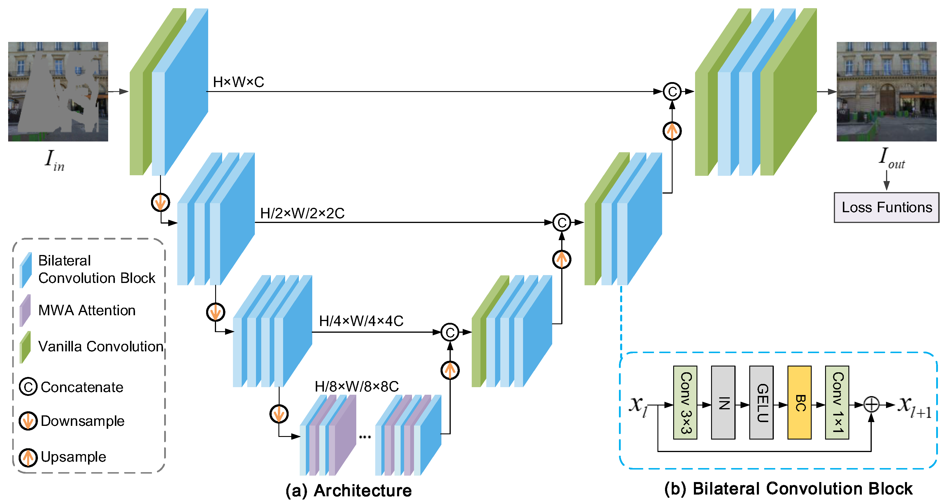
Learning-based image inpainting methods formulate the inpainting problem as a conditional image generation task [7]. Convolutional neural networks are commonly used to learn weights from massive datasets and predict the missing contents. Pathak et al. [7] first used the Generative Adversarial Network (GAN) to improve the semantic information of inpainting results. Some methods utilized auxiliary information as inpainting guidance and refined details, such as edges [46], structural information [47,48], semantic segmentation maps [49], and foreground object contours [50]; then, they refined the details. However, these methods often suffer from inconsistency in the generated structures and texture details due to the lack of the effective alignment of features in the two stages. Some researchers have utilized parallel networks [51] and recursive networks [52] to achieve powerful results. These methods have more parameters, making the training of models more time-consuming. Some pluralistic inpainting methods, such as VQ-VAE [48], PD-GAN [53], and PUT [54], were proposed to generate multiple completion images. In addition, standard convolution treats all features with the same kernel weights, which is unsuitable for the image completion of various corrupted areas. Some methods use modified convolution in different manners to address the inadaptability of corrupted and uncorrupted regions. For example, Partial Convolution (PC) [8] inferred missing pixels depending on valid pixels and automatically updated the valid region for the next layer; Gated Convolution (GC) [9] learned the feature selection mechanism for each channel and spatial location; and Dynamic Selection Network (DSN) [10] modified the deformable convolution to select valid information. Furthermore, some researchers [55,56] modified the instance normalization operation to adjust valuable features.

Furthermore, fully convolutional networks still lack the capacity to capture long-term relationships in distant contexts. The long-range correlation is vital because it is familiar to the human perception, which is sensitive to semantic relevance [57,58]. Yu et al. [17] proposed contextual attention to borrow features by matching patches from distant locations. Furthermore, other inpainting approaches [9,10,18,19,57,59] also integrated the attention operations into their networks to capture the long-term correlation, improving the inpainting performance.

3. Our Approach

This section demonstrates a bilateral convolution network for image inpainting, the architecture of which is shown in Figure 2a. Our inpainting network adopts a simple yet efficient one-stage U-Net architecture [23], and stacks a series of bilateral convolution blocks and MWA modules into the encoder and decoder. We first design a BC operator to propagate features using the surrounding information, considering distance. Then, we design a residual bilateral convolution block based on our proposed BC operator. Moreover, we introduce an MWA module to build multi-range dependencies for various scales of objects. Finally, we jointly optimize several loss functions to train the image completion network. The details of our network can be found in Appendix A.

3.1. Bilateral Convolution (BC)

3.1.1. Preliminaries

First, we explain why standard convolutions are inadaptable to corrupted and uncorrupted regions for image inpainting tasks. Theoretically, a convolution operation on the input features is defined as follows:

$$\begin{array}{cc}\hfill & \hfill F_{x,y}=\sum \sum W·I_{x,y},\hfill \end{array}$$

(1)

where $F_{x,y}\in {\mathbb{R}}^{C_{out}}$ represents the output map of the convolution operation located at $(x,y)$ in $C_{out}$ channels, $I_{x,y}\in {\mathbb{R}}^{C_{in}}$ is the input feature at $(x,y)$, W is the convolution filter weights with the dimensions $k_h\times k_w\times C_{in}\times C_{out}$, and $k_h$ and $k_w$ represent the kernel size. Here, the convolution bias is ignored. The equation shows that the same filter coefficients are applied at any spatial position in the standard convolution. This feature is suitable for tasks in which the input image is not treated differently, such as classification, detection, and segmentation. However, it is not suitable for inpainting tasks, for which the input consists of damaged and undamaged contexts.

Partial Convolution (PC) [8] conditions the completed results only in the valid regions, using the mask-update and re-normalization steps. This can be expressed as

$$\begin{array}{cc}\hfill & \hfill F_{x,y}=\left\{\begin{array}{cc}\hfill \beta \sum \sum W·\left(I·M\right),\hfill & \hfill \mathrm{if}sum\left(M\right)>0\hfill \\ 0,\hfill & \mathrm{otherwise}\hfill \end{array}\right.,\hfill \end{array}$$

(2)

where M is the corresponding binary mask in the convolution window; 1 represents a valid pixel, and 0 invalid. $\beta$ is the scaling factor, which equals the size of M divided by the sum of M elements. After the partial convolution operation, the mask is updated with the following rule:

$$M_{x,y}=\left\{\begin{array}{cc}\hfill 1,\hfill & \hfill \mathrm{if}sum\left(M\right)>0\hfill \\ \hfill 0,\hfill & \mathrm{otherwise}\hfill \end{array}\right..$$

(3)

Although PC improved the inpainting results, it still has some problems. The mask-update operation is too rough, being a binary hard update with a sliding window as the calculation unit, which cannot be smoothly propagated as a new mask layer by layer. If one valid pixel in the sliding window exists, this location mask value is updated as valid, as shown in the red edge windows of $M_{out}$ in Figure 3a. M has only one channel, and all F channels share the same non-smooth mask. These designs cause some propagation features to be invalid in the hole, as shown in the red box of F in Figure 3a, where some values are close to zero. Moreover, the rule-based update strategy is non-differential and also increases the difficulty of end-to-end learning.

Gated Convolution (GC) [9] improved PC by providing a learnable soft mask for each channel and each spatial location, defined as follows:

$$\begin{array}{cc}\hfill & M_{x,y}=\theta \left(\sum \sum W_m·I\right),\hfill \\ \hfill & {\tilde{F}}_{x,y}=\varphi \left(\sum \sum W_f·I\right),\hfill \\ \hfill & F_{x,y}={\tilde{F}}_{x,y}\odot M_{x,y},\hfill \end{array}$$

(4)

where $W_m$ and $W_f$ are two convolutional filters, $\theta$ is a sigmoid function that produces soft gating values $M_{x,y}\in {\mathbb{R}}^{C_{out}}$, $\varphi$ is an activation function, and ⊙ is element-wise multiplication. Yu et al. [9] showed that gating values could learn feature selection values to help generate higher-quality results. However, there is no strategy to obtain better features while the gating value is low. For example, some mask values are close to zero in the corrupted hole region, and due to the corresponding feature values also being invalid, as shown in the red box of F in Figure 3b.

3.1.2. Bilateral Convolution (BC)

We propose a BC operator for image inpainting networks; the architecture is shown in Figure 3c. The BC operator comprises the feature preservation term and propagation term. Both are based on the feature confidence level M. Specifically, the BC operator is similar to GC for feature selection. It uses a point-wise convolution and a $3\times 3$ depth-wise convolution with a Sigmoid activation function to compute its corresponding confidence map $M\in {\mathbb{R}}^{H\times W\times C}$, and then uses the confidence map to determine the feature preservation rate. This can be formulated as

$$\begin{array}{cc}\hfill & M=\theta \left(\sum \sum W_m·I\right),\hfill \\ \hfill & {\tilde{F}}_p=\varphi \left(\sum \sum W_f·I\right),\hfill \\ \hfill & F_p={\tilde{F}}_p\odot M,\hfill \end{array}$$

(5)

where $I\in {\mathbb{R}}^{H\times W\times C}$ is the input feature of the BC operator, and $\theta$ is the sigmoid activation function to ensure that the output confidence values are between 0 and 1. We use this soft gating value M to represent our confidence level, and a higher value in the corresponding position should contain a more helpful feature. $\varphi$ is an Instance Norm (IN) operator. $F_p$ is the preservation feature term, which means that a higher confidence level for the values of corresponding location features is better preserved.

The process of BC operator can be given as follows:

$$\begin{array}{cc}\hfill & F_g=\left(1-M\right)\odot \tilde{F},\hfill \\ \hfill & F=F_p+F_g,\hfill \end{array}$$

(6)

where $F_g$ is the propagation feature term; low confidence values in M represent unfavorable conditions for image inpainting and the requirement to propagate sufficient guidance.

As for the intermediate propagation feature $\tilde{F}$, inspired by diffusion-based approaches, we assume that every point in the features can be approximated from spatially close points. We execute convolution on the preservation feature $F_p$ with a Gaussian filter. The Gaussian filter measures the feature distance between it and the feature at the patch center. The Gaussian spatial function is defined as follows:

$$\begin{array}{c}\hfill G(x,y)=\frac{1}{2\pi }exp\left(\frac{x^2+y^2}{2{\sigma }^2}\right).\end{array}$$

(7)

With the help of Equation (7), we can obtain the intermediate propagation result $\tilde{F}$, reweighted by the feature distance. In our implementation, $\sigma$ = 1.

These designs of BC expand the receptive field and can dynamically adapt diverse corrupted regions of input. Furthermore, more valuable features can be preserved and propagated. For example, the output feature F shown in Figure 3c has higher, smoother values in the orange box and high-confidence values in the red box.

We adopt the residual block idea to design our bilateral convolution block. Its architecture is shown in Figure 2b. It can be expressed as follows:

$$\begin{array}{cc}\hfill & \hfill x_{l+1}=x_l+Conv\left(BC\left(\psi \left(Conv\left(x_l\right)\right)\right)\right),\hfill \end{array}$$

(8)

where $x_l$ and $x_{l+1}$ are the input and output of the l-th block, respectively, and $\psi$ represents the Instance Norm (IN) and the GELU activation function. Then, bilateral convolution BC dynamically adjusts the results of regular convolution to preserve features in valid positions and propagate new features with distance information in invalid positions.

3.2. Multi-Range Window Attention (MWA)

Many inpainting models [17,18,19,57,59] have integrated attention modules in order to mitigate the inefficiency of modeling the long-range dependencies of convolution neural networks. Although these models consider the similarity of deep features on the global spatial scale, they fail to build the dependencies between different scales of the feature [60], and the attention usually suffers from being over-concentrated and dispersed [20,61]. We note that some attention mechanisms for dividing windows in transformer architecture [21,60] provide a more efficient and favorable supervisory signal for modeling dependencies. In fact, an image often contains objects of various scales during inpainting tasks. Constructing the multi-range dependencies between different object features is beneficial when recovering the image. Motivated by this phenomenon, we propose the Multi-range Window Attention (MWA) to build dependencies among various feature ranges, as shown in Figure 4.

In the MWA module, we first split features into multiple heads along the channel. Then, we divide the split features of all heads into non-overlapped patches with different window sizes by window and shifted-window strategies. Specifically, when the window size is equal to the head’s feature size, it can obtain global attention. Self-attention only happens within each patch or window. Finally, we can obtain multi-range window attention via joint multi-branch attention.

The first step is splitting feature maps into multiple heads. We use a $1\times 1$ convolution to convert the feature $F_{in}\in {\mathbb{R}}^{H\times W\times C}$ to a new feature $F^{\prime }\in {\mathbb{R}}^{H\times W\times C^{\prime }}$, then split the new feature $F^{\prime }$ along the channel into several heads. These operations can be defined as follows:

$$\begin{array}{cc}\hfill & F^{\prime }=\sum \sum W_b·F_{in},\hfill \\ \hfill & \{F_1^{\prime },F_2^{\prime },\dots ,F_B^{\prime }\}=split\left(F^{\prime }\right),\hfill \end{array}$$

(9)

where $F_b^{\prime }\in {\mathbb{R}}^{H\times W\times d}$ is the feature on each head, $d=C^{\prime }/B$ is the channel of each head feature, and B is the total number of heads.

We introduce windows with different sizes to divide the feature maps into non-overlapping patches, which can cause each head of the various feature maps to have different range dependencies. For each window size, we deploy it on two head features. On one head feature, we execute normal window-based self-attention. On the other head feature, we execute shifted window-based self-attention, similar to Swin-Transformer [21]. After dividing the windows, each patch feature can be expressed as $F_{b,w}^{\prime }\in {\mathbb{R}}^{k_1\times k_2\times d}$, where $k_1\times k_2$ is the window size, $w\in \{1,2,\dots ,m\times n\}$ is the sequence number of the patches, and $m=H/k_1,n=W/k_2$. When $k_1=H$ and $k_2=W$, the patch is a global window.

Then, we compute self-attention within each patch, which includes three steps: embedding, matching, and attending [61]. We encode each patch feature map $F_{b,w}^{\prime }$ into a latent embedding space, which can be expressed as

$$\begin{array}{cc}\hfill & \hfill Q_{b,w}=\sum \sum W_{b,w}^q·F_{b,w}^{\prime },\hfill \\ \hfill & \hfill K_{b,w}=\sum \sum W_{b,w}^k·F_{b,w}^{\prime },\hfill \\ \hfill & \hfill V_{b,w}=\sum \sum W_{b,w}^v·F_{b,w}^{\prime },\hfill \end{array}$$

(10)

where $W_{b,w}^q,W_{b,w}^k$, and $W_{b,w}^v$ are three convolutions that map feature maps into the embedding space. $Q_{b,w}$, $K_{b,w}$, and $V_{b,w}$ are the query, key, and value features of patches in regular self-attention, respectively. The output of a window’s self-attention is calculated by

$$\begin{array}{cc}\hfill & \hfill Attention(Q_{b,w},K_{b,w},V_{b,w})=Softmax\left(\frac{Q_{b,w}{K}_{b,w}^T}{\sqrt{d}}\right)V_{b,w},\hfill \end{array}$$

(11)

where $\sqrt{d}$ is a scaling factor based on the dimension of feature maps. The matching operator is calculated by $Q_{b,w}{K}_{b,w}^T$ to obtain the attention map, which represents the correlation between all the tokens within the window. The attending operator performs a weighted summation of value features $V_{b,w}$ to obtain the output.

After determining self-attention in windows, we can obtain scale attention results for each joint window attention on each head. Specifically, we concatenate the attention results of the number of B branches. This jointly requires information from different window sizes and considers various range dependencies:

$$\begin{array}{cc}\hfill & \hfill F_a=Concatenate({WSA}_1,\dots ,{WSA}_B),\hfill \end{array}$$

(12)

where $F_a\in {\mathbb{R}}^{H\times W\times C^{\prime }}$, $C^{\prime }=Bd$, ${WSA}_b\in {\mathbb{R}}^{H\times W\times d}$ is the attention result representing jointed window attention on the b-th head. Next, we pass the concatenated result $F_a$ to a $3\times 3$ convolution to obtain the final result of multi-range window attention $F_{out}$.

In summary, with the help of multi-range local and global strategies on multiple heads, MWA can effectively borrow relevant features from different ranges, which better models the multi-range dependencies inside multi-range viewpoints.

We present the complexity analysis of our MWA module comparing multi-head self-attention [61]. In multi-head self-attention and our MWA, the same embedding operation is used; only the calculation cost in the matching operation is different. For simplicity, we only discuss the computation cost of the matching operation.

The shape of the input feature maps is $H\times W\times C$, where H and W are the height and width of feature maps, and C is the number of channels. The computation complexity of Global Self-Attention (GSA) is below:

$$\begin{array}{c}\hfill \mathcal{O}\left(GSA\right)=2{\left(HW\right)}^{2}C.\end{array}$$

(13)

The b-th head contains $m\times n$ windows, with a window size of $k_1=H/m$ and $k_2=W/n$. Then, the window self-attention cost of one head can be computed as follows:

$$\begin{array}{c}\hfill \mathcal{O}\left(WSA\right)=2\frac{{\left(HW\right)}^2}{mn}C=2k_1{k}_{2}HWC.\end{array}$$

(14)

From the above computation equations, when $k_1\ll H$ and $k_2\ll W$, the window self-attention of one head is more efficient, and the computation cost declines with $mn$ repetitions.

Our MWA includes one global self-attention head and several window self-attention heads with different window sizes. The computation cost is

$$\begin{array}{c}\hfill \mathcal{O}\left(GSA\right)+\sum _{b=1}^{B-1}\mathcal{O}\left({WSA}_b\right).\end{array}$$

(15)

The computation cost of multi-head self-attention with B heads is $B\times \mathcal{O}\left(GSA\right)$. MWA has $2HWC\times {\sum }_{b=1}^{B-1}(HW-k_{b,1}{k}_{b,2})$ lower complexity than multi-head self-attention [61]. Theoretically, the feature splits into many windows, $HW\ge k_{b,1}{k}_{b,2}$, so our MWA is more efficient than multi-head self-attention.

3.3. Loss Functions

Following some previous works [8,9,46,52], we train the networks with common loss functions to obtain high-quality and semantic levels of completed images, including adversarial loss [62], perceptual loss [63], style loss [62], and reconstruction loss [8]. We define the overall objective of our network as follows:

$$\begin{array}{cc}\hfill {\mathcal{L}}_{obj}\left(I_{gt},I_{out}\right)=& \hfill {\alpha }_a{\mathcal{L}}_a\left(I_{gt},I_{out}\right)+{\alpha }_p{\mathcal{L}}_p\left(I_{gt},I_{out}\right)+\hfill \\ \hfill & \hfill {\alpha }_s{\mathcal{L}}_s\left(I_{gt},I_{out}\right)+{\alpha }_r{\mathcal{L}}_r\left(I_{gt},I_{out}\right),\hfill \end{array}$$

(16)

where ${\mathcal{L}}_a$ is adversarial loss, ${\mathcal{L}}_p$ is perceptual loss, ${\mathcal{L}}_s$ is style loss, and ${\mathcal{L}}_r$ is reconstruction loss. $I_{gt}$ denotes the ground truth image. $I_{out}$ denotes the output of our network. ${\alpha }_a,{\alpha }_p,{\alpha }_s$, and ${\alpha }_r$ are the weights of each loss function.

We use the adversarial loss along with the Patch-GAN [62] to classify the recovery result $I_{out}$ and ground truth image $I_{gt}$. The adversarial loss can guide the model to produce more plausible and local details, which can be expressed as

$$\begin{array}{cc}\hfill & \hfill {\mathcal{L}}_a\left(I_{gt},I_{out}\right)={\mathbb{E}}_{I_{gt}}\left[logD\left(I_{gt}\right)\right]+{\mathbb{E}}_{I_{out}}\left[log\left[1D\left(I_{out}\right)\right]\right],\hfill \end{array}$$

(17)

where D is the discriminator network.

We use perceptual loss ${\mathcal{L}}_p$ to simulate the human perception of image quality. This method computes the $L_1$-norm distance on the high-level semantics features [63] and is expressed as follows:

$${\mathcal{L}}_p\left(I_{gt},I_{out}\right)=\sum _i{∥{\varphi }_{rel{u}_i}\left(I_{out}\right)-{\varphi }_{rel{u}_i}\left(I_{gt}\right)∥}_1,$$

(18)

where $\varphi$ is the VGG-19 classification model pre-trained on the ImageNet dataset [64], which can obtain the high-level semantics features. ${\varphi }_{rel{u}_i}$ is the activation map of the ith specified relu layer of VGG-19. In our training stage, ${\varphi }_i$ corresponds to layers relu1_1, relu2_1, relu3_1, relu4_1, and relu5_1 [63].

Since our network includes window-based attention and up-sampling operations, the checkerboard phenomenon often appears. Therefore, we use style loss to suppress this situation [65], computed by

$${\mathcal{L}}_s\left(I_{gt},I_{out}\right)=\sum _i{∥{\varphi }_{rel{u}_i}\left(I_{out}\right){\varphi }_{rel{u}_i}^T\left(I_{out}\right)-{\varphi }_{rel{u}_i}\left(I_{gt}\right){\varphi }_{rel{u}_i}^T\left(I_{gt}\right)∥}_1,$$

(19)

where $\varphi$ is the same as the VGG-19 model in perceptual loss, ${\varphi }_{rel{u}_i}{\varphi }_{rel{u}_i}^T$ is a Gram matrix constructed by activation maps ${\varphi }_{rel{u}_i}$, and ${\varphi }_{rel{u}_i}$ are activation maps from relu2_2, relu3_4, relu4_4, and relu5_2 in the VGG-19 model [62].

The reconstruction loss is calculated by the $L_1$-norm distance between the output $I_{out}$ and the ground truth $I_{gt}$ at the pixel level [8], defined as

$$\begin{array}{c}\hfill {\mathcal{L}}_r\left(I_{gt},I_{out}\right)={\parallel I_{out}-I_{gt}\parallel }_1.\end{array}$$

(20)

4. Experiments

This section reports the details of our inpainting network’s experimental datasets, settings, and model training.

4.1. Datasets

In image inpainting tasks, three remote sensing image datasets, three typical image inpainting datasets, and one cloud removal dataset were used.

The three RS image datasets were AID [66], NWPU-RESISC45 [67], and PatternNet [11], and their descriptions are as follows:

• The AID dataset was released by Wuhan University, containing data extracted from different Google Earth sensors [66]. It contains 10,000 RS images with 30 scene categories. We used 500 images for testing, with approximately 17 images in each category.
• The NWPU-RESISC45 dataset was released by Northwestern Polytechnical University containing data extracted from Google Earth [67]. It includes 31,500 images with 45 scene categories. We selected 500 images for testing, with approximately 11 images in each category.
• PatternNet is a remote sensing image dataset with 256 × 256 resolution. It mainly obtains 38 scenes with 30,400 images from Google Earth imagery or the Google Map API [11]. We used 400 images for testing, including 10 or 11 images of each scene.

Three typical image inpainting datasets include Paris StreetView [12], CelebA-HQ [68], and Places2 [13], and their introductions are as follows:

• The Paris StreetView dataset contains images of Paris from Google StreetView. It mainly contains the structural information of windows, doors, and buildings, and has 14,900 training images and 100 test images [12].
• The CelebA-HQ dataset mainly consists of celebrity faces and includes 30,000 images [68]. We used the first 2000 images as the test set. This dataset is a high-quality version of the CelebA dataset [69].
• The Places2 dataset was released by MIT. It contains over 1.8 million training images from over 365 scenes [13]. We randomly selected 4000 images from the original validation set for testing.

The cloud removal dataset is the Remote sensing Image Cloud rEmoving dataset (RICE) [70], which consists of RICE1 and RICE2. The RICE2 dataset contains 736 images from the Landsat 8 OLI/TIRS dataset. We randomly selected 630 images for training and 106 images for testing.

Furthermore, in the image completion task, when verifying the algorithm, we need to determine the location of damaged regions. Therefore, we utilized the irregular mask dataset from PC [8] as the test mask dataset. This dataset contains six groups of masks with different ratios of mask regions, and there are 2000 images in each group.

4.2. Experimental Setting

We trained our network on a single RTX3090 GPU with a batch size of eight images. We used the AdamW optimizer with betas $(0.5,0.9)$. We set an initial learning rate of ${10}^{-4}$, then decreased it to ${10}^{-5}$ for the fine-tuning of the model. For the weights of each loss function, we set ${\alpha }_a=0.1,{\alpha }_p=0.1,{\alpha }_s=250,{\alpha }_r=1$ to train the joint optimization of the loss functions, with reference to previous methods [46,51]. We employed $B=5$ attention heads, and the dimension feature map of each branch d was 32. We set the window sizes as 8 and 16 for the local window and shift window attention heads, and set the window size on the global attention head as 64. For AID, NWPU-RESISC45, PatternNet, and Paris StreetView, we trained and fine-tuned our model for 70 epochs. For CelebA-HQ, we trained and fine-tuned our model for 100 and 50 epochs, respectively. As for Places2, we trained our model for four epochs and fine-tuned it for two epochs. The input images of our model were $256\times 256$. Following previous inpainting works [8], we also employ PSNR (Peak Signal-to-Noise Ratio), SSIM (Structural Similarity Index Measure), and FID (Fréchet Inception Distance) to quantitatively compare our results with SOTA methods.

4.3. Comparison Models

We compared our network with several state-of-the-art inpainting methods, including Partial Convolution (PC) [8], Gated Convolution (GC) [9], Recurrent Feature Reasoning Network (RFR) [52], Dynamic Selection Network (DSN) [10], PUT [54], and SpA-GAN [40]. Some of these methods are similar to solving the inadaptability of random corrupted regions of convolution, and some match the good performance of the inpainting model:

• PC [8]: An encoder–decoder inpainting model that adopts a rule-based updating mask, renormalized only on valid pixels in the U-Net architecture;
• GC [9]: A two-stage inpainting model representing an improvement on the PC model, having learned a dynamic gating mask. This model can achieve better inpainting results;
• DSN [10]: A two-parallel U-Net inpainting model used to validate migratable convolution and regional composite normalization in order to select valid information dynamically;
• RFR [52]: A recurrent encoder–decoder inpainting model adopting the partial convolution of U-Net architecture, which recurrently gathers the hole boundary features and recovers structures to strengthen the results;
• PUT [54]: A pluralistic inpainting model adopting the patch-based VQVAE without downsampling, using a transformer without quantization to reduce information loss;
• SpA-GAN [40]: The SpA-GAN model uses the spatial attention generative adversarial network to recover the corrupted or cloud obscuration regions and generate realistic images of remotely sensed scenes.

5. Results

In this section, we compare our results with state-of-the-art methods, both qualitatively and quantitatively, on five datasets. Then, we conduct experiments on actual clouded scenario images to remove the clouds. Next, we analyze the training loss of our network. We also present ablation studies to validate the effectiveness of our proposed BC block and MWA module.

5.1. Quantitative Comparison

We quantitatively compare our network with comparison models in terms of SSIM, PSNR, and FID.

Table 1. Numerical comparison of the AID and NWPU-RESISC45 datasets.

Dataset		AID							NWPU-RESISC45
Metrics	Mask Ratio	PC	GC	RFR	DSN	PUT	SpA-GAN	Ours	PC	GC	RFR	DSN	PUT	SpA-GAN	Ours
FID ↓	10–20%	55.56	39.05	31.04	20.77	20.29	52.29	16.86	46.39	31.73	25.53	17.13	14.97	41.34	13.09
	20–30%	83.30	65.28	45.95	35.75	34.04	79.62	28.04	70.60	54.56	33.35	29.02	24.86	64.03	22.32
	30–40%	106.24	87.61	58.14	48.56	45.65	106.75	38.03	90.10	75.61	41.39	40.42	33.79	83.93	30.76
	40–50%	122.87	114.62	72.28	61.35	56.85	130.71	48.14	107.52	100.11	51.23	51.70	43.19	108.64	40.29
	AVG	91.99	76.64	51.85	41.61	39.21	92.34	32.77	78.65	65.50	37.88	34.57	29.20	74.49	26.62
SSIM ↑	10–20%	0.809	0.904	0.887	0.917	0.915	0.835	0.920	0.819	0.916	0.905	0.931	0.931	0.862	0.935
	20–30%	0.672	0.826	0.822	0.845	0.841	0.717	0.851	0.695	0.847	0.858	0.868	0.865	0.769	0.877
	30–40%	0.550	0.742	0.742	0.763	0.754	0.593	0.772	0.579	0.766	0.788	0.791	0.786	0.659	0.806
	40–50%	0.436	0.644	0.646	0.670	0.657	0.461	0.681	0.457	0.668	0.699	0.699	0.691	0.528	0.717
	AVG	0.617	0.779	0.774	0.799	0.792	0.652	0.806	0.638	0.799	0.813	0.822	0.818	0.705	0.834
PSNR ↑	10–20%	23.67	28.31	27.39	28.96	28.65	24.90	29.05	24.32	29.36	28.56	30.14	30.02	26.26	30.43
	20–30%	20.61	25.65	25.18	26.05	25.77	22.13	26.27	21.44	26.68	26.62	27.18	26.97	23.77	27.52
	30–40%	18.65	23.91	23.59	24.16	23.79	19.90	24.35	19.39	24.83	24.90	25.08	24.81	21.48	25.47
	40–50%	17.23	22.48	22.21	22.68	22.21	17.88	22.81	17.75	23.31	23.39	23.43	23.06	19.31	23.75
	AVG	20.04	25.09	24.59	25.46	25.11	21.20	25.62	20.73	26.05	25.87	26.46	26.22	22.71	26.79

The ↓ indicates lower is better, while ↑ indicates higher is better. The bold number indicates that it has the best metric value compared with other methods on the same dataset.

,

Table 2. Numerical comparison of the PatternNet and Paris StreetView datasets.

Dataset		PatternNet							Paris StreetView
Metrics	Mask Ratio	PC	GC	RFR	DSN	PUT	SpA-GAN	Ours	PC	GC	RFR	DSN	PUT	SpA-GAN	Ours
FID ↓	10–20%	53.63	27.48	33.79	17.33	14.15	39.78	12.72	63.78	20.69	20.33	16.28	15.14	37.70	13.29
	20–30%	82.55	49.46	48.77	28.85	23.28	64.95	21.60	102.11	39.48	28.93	29.39	27.57	63.49	23.32
	30–40%	105.78	72.84	62.81	42.58	32.76	94.60	29.98	131.91	58.66	39.84	42.02	38.85	85.08	34.14
	40–50%	128.51	97.72	76.61	54.16	41.31	124.08	39.74	158.82	82.51	49.96	53.66	49.56	114.18	46.83
	AVG	92.62	61.88	55.50	35.73	27.88	80.85	26.01	114.16	50.34	34.77	35.34	32.78	75.11	29.40
SSIM ↑	10–20%	0.822	0.930	0.898	0.933	0.937	0.877	0.939	0.843	0.952	0.943	0.952	0.956	0.907	0.960
	20–30%	0.696	0.872	0.841	0.875	0.881	0.783	0.887	0.730	0.915	0.908	0.914	0.913	0.837	0.926
	30–40%	0.580	0.797	0.766	0.803	0.813	0.672	0.822	0.622	0.865	0.861	0.859	0.857	0.742	0.877
	40–50%	0.456	0.700	0.673	0.718	0.734	0.541	0.742	0.498	0.792	0.799	0.791	0.791	0.608	0.812
	AVG	0.639	0.825	0.795	0.832	0.841	0.718	0.848	0.673	0.881	0.878	0.879	0.879	0.774	0.894
PSNR ↑	10–20%	24.00	29.66	27.84	29.76	29.98	26.39	30.32	24.06	31.52	30.18	31.06	31.71	27.59	32.13
	20–30%	21.12	27.05	25.79	26.91	27.05	23.68	27.53	21.02	28.50	27.76	28.05	28.25	24.82	29.18
	30–40%	19.13	24.90	24.02	24.66	24.86	21.33	25.28	19.02	26.03	25.99	25.92	26.06	22.37	26.87
	40–50%	17.47	23.17	22.55	23.05	23.20	19.16	23.59	17.14	24.80	24.25	24.05	24.15	19.71	24.87
	AVG	20.43	26.20	25.05	26.10	26.27	22.64	26.68	20.31	27.71	27.05	27.27	27.54	23.62	28.26

The ↓ indicates lower is better, while ↑ indicates higher is better. The bold number indicates that it has the best metric value compared with other methods on the same dataset.

and

Table 3. Numerical comparison of the CelebA-HQ and Places2 datasets.

Dataset		CelebA-HQ						Places2
Metrics	Mask Ratio	PC	GC	RFR	DSN	PUT	Ours	PC	GC	RFR	DSN	PUT	Ours
FID ↓	10–20%	9.20	2.54	5.17	1.91	1.87	1.42	11.27	5.57	5.23	3.63	4.19	2.90
	20–30%	18.53	4.49	4.06	3.18	3.21	2.43	22.02	10.67	6.58	6.28	7.65	4.92
	30–40%	34.63	6.84	4.89	4.70	4.57	3.58	35.73	17.60	8.64	9.59	12.00	6.96
	40–50%	56.45	9.83	6.11	6.20	5.80	4.70	53.01	27.80	12.00	13.71	16.93	9.43
	AVG	29.70	5.93	5.06	4.00	3.86	3.03	30.51	15.41	8.11	8.30	10.19	6.05
SSIM ↑	10–20%	0.925	0.979	0.969	0.981	0.978	0.983	0.880	0.951	0.937	0.954	0.945	0.956
	20–30%	0.860	0.959	0.958	0.963	0.958	0.966	0.791	0.906	0.903	0.910	0.889	0.914
	30–40%	0.785	0.931	0.939	0.939	0.929	0.944	0.700	0.852	0.858	0.856	0.822	0.863
	40–50%	0.699	0.896	0.913	0.910	0.895	0.916	0.600	0.784	0.797	0.791	0.742	0.798
	AVG	0.817	0.941	0.945	0.948	0.940	0.952	0.743	0.873	0.874	0.878	0.850	0.883
PSNR ↑	10–20%	25.50	32.26	30.93	32.72	32.10	33.13	23.16	28.57	27.34	28.51	27.42	28.72
	20–30%	22.21	29.10	28.94	29.53	28.81	29.93	20.23	25.46	24.99	25.32	24.06	25.53
	30–40%	19.78	26.71	27.11	27.15	26.34	27.48	18.24	23.33	23.15	23.12	21.74	23.32
	40–50%	17.87	24.78	25.47	25.34	24.43	25.55	16.62	21.53	21.47	21.33	19.84	21.45
	AVG	21.34	28.21	28.11	28.69	27.92	29.02	19.56	24.72	24.24	24.57	23.27	24.76

The ↓ indicates lower is better, while ↑ indicates higher is better. The bold number indicates that it has the best mertic value compared with other methods on the same dataset.

show the results with different corruption ratios on the AID, NWPU-RESISC45, PatternNet, Paris StreetView, CelebA-HQ, and Places2 datasets, respectively. The best results in each group are highlighted in bold. The ↓ indicates that a lower value is better, while ↑ indicates that higher is better. The quantitative results show that our network has comparable performance against other comparison models and produces the best evaluation results on FID and SSIM. Compared with DSN, our method increases the average value of FID (27.0%, 29.9%, 37.4%, 20.2%, 31.8%, and 37.2%), the average value of SSIM (0.9%, 1.4%, 1.8%, 1.65%, 0.4%, and 0.6%), and the average value of PSNR (0.6%, 1.3%, 2.2%, 3.5%, 1.1%, and 0.7%) on AID, NWPU-RESISC45, PatternNet, Paris, CelebA-HQ, and Places2, respectively. Compared with PUT, our method increases the average value of FID (19.7%, 9.7%, 7.2%, 11.5%, 27.4%, 68.4%), the average value of SSIM (1.77%, 1.9%, 0.74%, 1.62%, 1.29%, 3.77%), and the average value of PSNR (2%, 2.2%, 1.5%, 2.5%, 3.8%, 6.0%) on AID, NWPU-RESISC45, PatternNet, Paris, CelebA-HQ, and Places2, respectively. These results show that our method has greatly improved FID metrics and produces better completion results for the surrounding features with distance and multi-range dependencies.

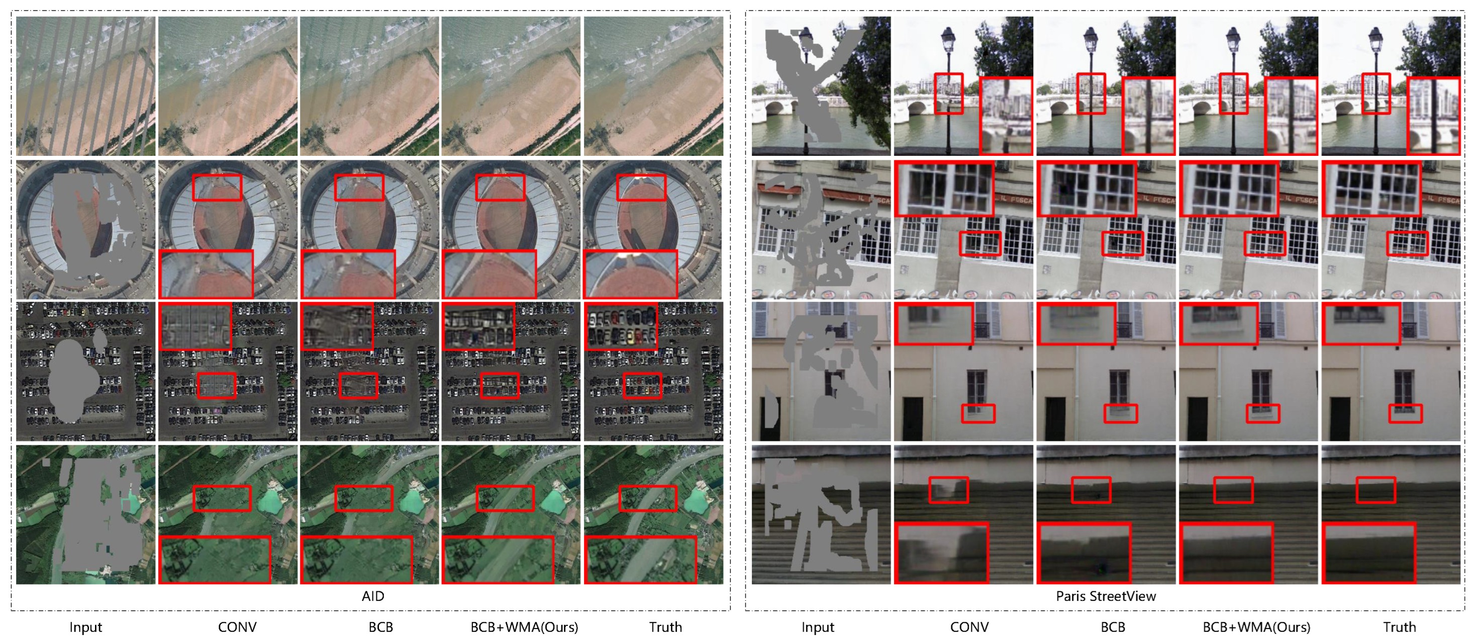
5.2. Qualitative Comparison

We also provide some qualitative comparisons to intuitively analyze the results of different methods. Figure 5 and Figure 6 show the results of the visual comparison of our method and six state-of-the-art methods on remote sensing and natural datasets. For each dataset, the results in the first two rows are the overall completion quality, and the results in the last two rows are the local details displayed in the red box. PC [8], based on the rule-based mask-update method, is unable to obtain valid information to fill the middle part of the hole. Especially for images with large holes, regions are filled with over-saturated and structurally distorted patches. GC [9], based on the learnable feature selection module, can obtain color consistency results but easily generate blurry content. The completed images produced by RFR [52] are relatively good. However, this method still suffers from inconsistent structures, e.g., the blurry bridges of AID and PatternNet, some breaking of the window railings in the third row of Paris StreetView, and a missing human ear in the fourth row of CelebA-HQ. DSN [10] can complete some good images, but it misses some content at the object edge. For example, the car and the human ear lose some content in Paris StreetView and CelebA-HQ, respectively. PUT [54] produces inconsistent contents, incontinuous edges, and abnormal colors, e.g., the windows, railings, and stairs of the buildings in Paris StreetView and Places2. SpA-GAN [40] can restore small damaged regions but cannot process large damaged regions, and some completion results have inconsistent content.

Compared with these methods, our network results in rich texture, consistent structure, and intact objects on both remote sensing and natural images. For example, rich texture as a result of our method is shown in the excellent brick texture of the buildings and the continual window fence of Paris StreetView, the natural hair covering the eye of CelebA-HQ, and the continuous cabinet door strip of Places2. Consistent structure is shown in the buildings of the RS results, the two consistent eyes of CelebA-HQ, and the steps of Places2. Intact objects are shown in the intact bridge of AID and PatternNet, the intact car of Paris StreetView, the intact ear of CelebA-HQ, and the intact red ball of Places2.

5.3. Experiments of Cloud Removal on Real Images

We conducted cloud removal experiments on RICE2 [70] to verify the performance of our network on real data. We trained our bilateral convolution network for 200 epochs and fine-tuned 70 epochs, and compared our cloud removal results with SpA-GAN [40], as shown in

Table 4. Numerical comparison of cloud removal on the RICE2 dataset.

Models	FID ↓	SSIM ↑	PSNR ↑
SpA-GAN	45.44	0.731	29.74
Ours	39.68	0.789	30.97

The ↓ indicates lower is better, while ↑ indicates higher is better. The bold number indicates that it has the best metric value compared with other methods.

and Figure 7. The quantitative results show that our network performs better than SpA-GAN on the cloud removal RICE2 dataset. The visual results in Figure 7 show that our model achieves rich texture and consistent structure in bareland and grassland scenes. However, the SpA-GAN results suffer from blurring, ghosting, and artifact problems.

5.4. Loss Analysis

In order to analyze the training process of our network, the training loss curves on four datasets are shown in Figure 8. It can be seen that reconstruction loss, perceptual loss, and style loss decrease with the increase in the number of training epochs. The Patch-GAN generator and discriminator network adversarially learn from each other, which leads the adversarial loss to fluctuate. This situation is in line with the training process of the GAN network. These four losses constitute our objective loss, and the value of the objective loss is shown to be declining in Figure 8, which shows that the network can continue to learn until the convergence state. Furthermore, it can be seen from the objective loss curves that the objective loss stabilizes in the range of the 60th epoch, while it decreases after the 70th epoch. This is because the fine-tuning stage starts in the 70th epoch, which shows that adjusting the learning rate during this stage is helpful to the training process.

5.5. Ablation Studies

To better analyze the impact of the BC block and MWA module in our network, we perform ablation studies on the AID and Paris StreetView datasets. The designs of the experiments are as follows:

• Two experiments are conducted to analyze the effectiveness of the BC block. The first experiment is denoted as “CONV”, which replaces each layer with standard convolution operators in our designed U-Net style network. The second experiment is denoted as “BC”, which uses the proposed BC block of each layer in our network.
• Two experiments are conducted to validate the effectiveness of the MWA. The “w/ CA” experiment consists of replacing the MWA in our network with the contextual attention (CA) [17]. The “w/o g” experiment consists of replacing the header of the global attention with a window attention of size 8 in MWA.

All networks mentioned above have the same number of layers and loss functions. The details of our network are shown in Appendix A. The quantitative results of the ablation experiments are displayed in

Table 5. Analysis of the BC block network on the AID and Paris StreetView datasets.

Dataset	AID						Paris StreetView
Metrics	FID ↓		SSIM ↑		PSNR ↑		FID ↓		SSIM ↑		PSNR ↑
Mask Ratio	CONV	BC	CONV	BC	CONV	BC	CONV	BC	CONV	BC	CONV	BC
10–20%	22.59	18.81	0.905	0.914	28.12	28.69	16.76	13.44	0.951	0.958	31.05	31.95
20–30%	37.47	31.98	0.830	0.842	25.48	25.94	31.28	24.09	0.911	0.923	28.09	28.98
30–40%	51.09	43.36	0.744	0.759	23.69	24.05	45.38	34.96	0.847	0.872	25.69	26.72
40–50%	64.89	55.82	0.644	0.662	22.16	22.50	61.88	46.07	0.763	0.807	23.48	24.71
AVG	44.01	37.49	0.781	0.794	24.86	25.30	38.83	29.64	0.868	0.890	27.08	28.09

The ↓ indicates lower is better, while ↑ indicates higher is better. The bold number indicates that it has the best metric value compared with other methods on the same dataset.

and

Table 6. Analysis of the MWA module on the AID and Paris StreetView datasets.

Dataset	AID									Paris StreetView
Metrics	FID ↓			SSIM ↑			PSNR ↑			FID ↓			SSIM ↑			PSNR ↑
Mask Ratio	w/ CA	w/o g	Ours	w/ CA	w/o g	Ours	w/ CA	w/o g	Ours	w/ CA	w/o g	Ours	w/ CA	w/o g	Ours	w/ CA	w/o g	Ours
10–20%	20.62	17.09	16.86	0.912	0.917	0.920	28.51	28.84	29.05	14.45	13.55	13.29	0.957	0.959	0.960	31.74	32.06	32.13
20–30%	35.12	28.24	28.04	0.837	0.847	0.851	25.77	26.09	26.27	26.57	24.60	23.32	0.921	0.925	0.926	28.81	29.13	29.18
30–40%	47.61	38.73	38.03	0.753	0.767	0.772	23.91	24.19	24.35	37.58	34.80	34.14	0.866	0.875	0.877	26.46	26.78	26.87
40–50%	60.91	48.84	48.14	0.655	0.673	0.681	22.37	22.64	22.81	50.04	48.18	46.83	0.796	0.807	0.812	24.38	24.75	24.87
AVG	41.07	33.23	32.77	0.789	0.801	0.806	25.14	25.44	25.62	32.16	30.29	29.39	0.885	0.892	0.894	27.85	28.18	28.26

The ↓ indicates lower is better, while ↑ indicates higher is better. The bold number indicates that it has the best metric value compared with other methods on the same dataset.

, and the corresponding qualitative results are shown in Figure 9.

5.5.1. Effectiveness of the BC Block

The proposed BC block is a residual block that includes bilateral convolution. This convolution is composed of the feature preservation term and propagation term. To evaluate the effects of the proposed BC block on inpainting, we replace all standard convolution operators with the BC blocks in our designed U-Net style network. We denote the standard convolution as CONV.

Comparing the quantitative metrics of the CONV and BC block networks in Table 5, the BC block network generates better results than the CONV network. Furthermore, the visual results of the BC block network are better than those of the CONV network, as shown in Figure 9. These results demonstrate that our BC block can preserve better features, and propagate new features with distance information. Therefore, these characteristics are indeed suitable and beneficial for image inpainting.

5.5.2. Effectiveness of the MWA

We compare our MWA with CA and without the global header (w/o g). The experimental results are shown in Table 6. Compared with CA, we achieved higher scores when using the MWA module. This shows that our multi-range window strategy can capture more features that are suitable for completion than the global contextual attention. Compared with the “w/o g” model, this shows that global dependency is still needed in the image restoration task.

Comparing the BC column of Table 5 with the column representing our method in Table 6, we find that our method performs better than using only the BC block. Furthermore, our model can generate more real textures than using only the BC block, as exemplified by our results in Figure 9 for the AID dataset (the dead-line recovery result (row 1), the circle stadium (row 2), the cars in the parking (row 3), the continuity river (row 4)) and in Figure 9 for the Paris StreetView dataset (the bridge hole behind the tree (row 1), the continuous window fence and edge (rows 2 and 3), and the building’s edge (row 4)). These visual results show that our proposed MWA attention can capture multiple ranges of dependencies among pixels and improve the integrity and consistency of the inpainted contents.

6. Conclusions

In this paper, we customize a bilateral convolution network to reconstruct corrupted images, which stacks a series of BC blocks and MWA modules. With the BC operator, the BC block could simultaneously consider the reliability of features based on the spatial location and the feature value, which could be used to adaptively handle diverse corrupted regions and efficiently preserve and propagate information from known regions to unknown regions. Furthermore, the MWA with multi-range window self-attention can model different ranges of spatial dependencies among pixels. The results of quantitative and qualitative experiments on typical remote sensing datasets and image inpainting datasets demonstrate that our network is robust to various scene images and generates more appropriate and consistent content than several state-of-the-art methods. However, our BC operator has the limitation of using a Gaussian filter with a static kernel, which may not work well on large damaged regions. In future studies, we will consider using deformable convolution to expand the receptive field of the Gaussian kernel and convolution kernel, which may help to generate satisfactory completion results on various complex damaged images.

References

1. Shen, H.; Li, X.; Cheng, Q.; Zeng, C.; Yang, G.; Li, H.; Zhang, L. Missing information reconstruction of remote sensing data: A technical review. IEEE Geosci. Remote Sens. Mag. 2015, 3, 61–85. [Google Scholar] [CrossRef]
2. Shao, M.; Wang, C.; Wu, T.; Meng, D.; Luo, J. Context-based multiscale unified network for missing data reconstruction in remote sensing images. IEEE Geosci. Remote Sens. Lett. 2020, 19, 1–5. [Google Scholar] [CrossRef]
3. Ng, M.K.P.; Yuan, Q.; Yan, L.; Sun, J. An adaptive weighted tensor completion method for the recovery of remote sensing images with missing data. IEEE Trans. Geosci. Remote Sens. 2017, 55, 3367–3381. [Google Scholar] [CrossRef]
4. Zhao, H.; Duan, S.; Liu, J.; Sun, L.; Reymondin, L. Evaluation of five deep learning models for crop type mapping using sentinel-2 time series images with missing information. Remote Sens. 2021, 13, 2790. [Google Scholar] [CrossRef]
5. Bertalmio, M.; Sapiro, G.; Caselles, V.; Ballester, C. Image inpainting. In Proceedings of the 27th Annual Conference on Computer Graphics and Interactive Techniques, New Orleans, LA, USA, 23–28 July 2000; pp. 417–424. [Google Scholar]
6. Gao, Y.; Sun, X.; Liu, C. A General Self-Supervised Framework for Remote Sensing Image Classification. Remote Sens. 2022, 14, 4824. [Google Scholar] [CrossRef]
7. Pathak, D.; Krahenbuhl, P.; Donahue, J.; Darrell, T.; Efros, A.A. Context Encoders: Feature Learning by Inpainting. In Proceedings of the 2016 IEEE Conference on Computer Vision and Pattern Recognition (CVPR), Las Vegas, NV, USA, 27–30 June 2016. [Google Scholar]
8. Liu, G.; Reda, F.A.; Shih, K.J.; Wang, T.C.; Tao, A.; Catanzaro, B. Image Inpainting for Irregular Holes Using Partial Convolutions. In Proceedings of the European Conference on Computer Vision (ECCV), Munich, Germany, 8–14 September 2018; pp. 85–100. [Google Scholar]
9. Yu, J.; Lin, Z.; Yang, J.; Shen, X.; Lu, X.; Huang, T.S. Free-form image inpainting with gated convolution. In Proceedings of the IEEE/CVF International Conference on Computer Vision, Seoul, Republic of Korea, 27 October–2 November 2019; pp. 4471–4480. [Google Scholar]
10. Wang, N.; Zhang, Y.; Zhang, L. Dynamic selection network for image inpainting. IEEE Trans. Image Process. 2021, 30, 1784–1798. [Google Scholar] [CrossRef] [PubMed]
11. Zhou, W.; Newsam, S.; Li, C.; Shao, Z. PatternNet: A benchmark dataset for performance evaluation of remote sensing image retrieval. ISPRS J. Photogramm. Remote Sens. 2018, 145, 197–209. [Google Scholar] [CrossRef] [Green Version]
12. Doersch, C.; Singh, S.; Gupta, A.; Sivic, J.; Efros, A. What makes paris look like paris? ACM Trans. Graph. 2012, 31, hal-01053876. [Google Scholar] [CrossRef]
13. Zhou, B.; Lapedriza, A.; Khosla, A.; Oliva, A.; Torralba, A. Places: A 10 Million Image Database for Scene Recognition. IEEE Trans. Pattern Anal. Mach. Intell. 2018, 40, 1452–1464. [Google Scholar] [CrossRef] [Green Version]
14. Liu, H.; Jiang, B.; Song, Y.; Huang, W.; Yang, C. Rethinking image inpainting via a mutual encoder-decoder with feature equalizations. In Computer Vision–ECCV 2020, Proceedings of the European Conference on Computer Vision (ECCV), Glasgow, UK, 2–28 August 2020; Springer: Cham, Switzerland, 2020; pp. 725–741. [Google Scholar]
15. Ballester, C.; Bertalmio, M.; Caselles, V.; Sapiro, G.; Verdera, J. Filling-in by joint interpolation of vector fields and gray levels. IEEE Trans. Image Process. 2001, 10, 1200–1211. [Google Scholar] [CrossRef] [PubMed]
16. Tomasi, C.; Manduchi, R. Bilateral filtering for gray and color images. In Proceedings of the Sixth International Conference on Computer Vision, Bombay, India, 7 January 1998; pp. 839–846. [Google Scholar]
17. Yu, J.; Lin, Z.; Yang, J.; Shen, X.; Lu, X.; Huang, T.S. Generative Image Inpainting with Contextual Attention. In Proceedings of the IEEE/CVF Conference on Computer Vision and Pattern Recognition (CVPR), Salt Lake City, UT, USA, 18–23 June 2018. [Google Scholar]
18. Zeng, Y.; Fu, J.; Chao, H.; Guo, B. Learning Pyramid-Context Encoder Network for High-Quality Image Inpainting. In Proceedings of the IEEE/CVF Conference on Computer Vision and Pattern Recognition (CVPR), Long Beach, CA, USA, 15–20 June 2019. [Google Scholar]
19. Liu, H.; Jiang, B.; Xiao, Y.; Yang, C. Coherent Semantic Attention for Image Inpainting. In Proceedings of the IEEE/CVF International Conference on Computer Vision (ICCV), Seoul, Republic of Korea, 27 October–2 November 2019. [Google Scholar]
20. Yang, R.; Ma, H.; Wu, J.; Tang, Y.; Xiao, X.; Zheng, M.; Li, X. ScalableViT: Rethinking the Context-oriented Generalization of Vision Transformer. arXiv 2022, arXiv:2203.10790. [Google Scholar]
21. Liu, Z.; Lin, Y.; Cao, Y.; Hu, H.; Wei, Y.; Zhang, Z.; Lin, S.; Guo, B. Swin transformer: Hierarchical vision transformer using shifted windows. In Proceedings of the IEEE/CVF International Conference on Computer Vision (ICCV), Montreal, QC, Canada, 10–17 October 2021; pp. 10012–10022. [Google Scholar]
22. Vaswani, A.; Ramachandran, P.; Srinivas, A.; Parmar, N.; Hechtman, B.; Shlens, J. Scaling local self-attention for parameter efficient visual backbones. In Proceedings of the IEEE/CVF Conference on Computer Vision and Pattern Recognition (CVPR), Nashville, TN, USA, 20–25 June 2021; pp. 12894–12904. [Google Scholar]
23. Ronneberger, O.; Fischer, P.; Brox, T. U-net: Convolutional networks for biomedical image segmentation. In Medical Image Computing and Computer-Assisted Intervention—MICCAI 2015, Proceedings of the International Conference on Medical Image Computing and Computer-Assisted Intervention, Munich, Germany, 5–9 October 2015; Springer: Cham, Switzerland, 2015; pp. 234–241. [Google Scholar]
24. Li, X.; Shen, H.; Zhang, L.; Zhang, H.; Yuan, Q. Dead pixel completion of aqua MODIS band 6 using a robust M-estimator multiregression. IEEE Geosci. Remote Sens. Lett. 2013, 11, 768–772. [Google Scholar]
25. Wang, Q.; Wang, L.; Li, Z.; Tong, X.; Atkinson, P.M. Spatial–spectral radial basis function-based interpolation for Landsat ETM+ SLC-off image gap filling. IEEE Trans. Geosci. Remote Sens. 2020, 59, 7901–7917. [Google Scholar] [CrossRef]
26. Zeng, C.; Shen, H.; Zhang, L. Recovering missing pixels for Landsat ETM+ SLC-off imagery using multi-temporal regression analysis and a regularization method. Remote Sens. Environ. 2013, 131, 182–194. [Google Scholar] [CrossRef]
27. Li, X.; Shen, H.; Zhang, L.; Zhang, H.; Yuan, Q.; Yang, G. Recovering quantitative remote sensing products contaminated by thick clouds and shadows using multitemporal dictionary learning. IEEE Trans. Geosci. Remote Sens. 2014, 52, 7086–7098. [Google Scholar]
28. Siu, W.C.; Hung, K.W. Review of image interpolation and super-resolution. In Proceedings of the Asia Pacific Signal and Information Processing Association Annual Summit and Conference, Hollywood, CA, USA, 3–6 December 2012; pp. 1–10. [Google Scholar]
29. Criminisi, A.; Perez, P.; Toyama, K. Region Filling and Object Removal by Exemplar-Based Image Inpainting. IEEE Trans. Image Process. 2004, 13, 1200–1212. [Google Scholar] [CrossRef]
30. Barnes, C.; Shechtman, E.; Finkelstein, A.; Goldman, D.B. PatchMatch: A randomized correspondence algorithm for structural image editing. ACM Trans. Graph. 2009, 28, 24–35. [Google Scholar] [CrossRef]
31. Chan, T.F.; Shen, J. Nontexture inpainting by curvature-driven diffusions. J. Vis. Commun. Image Represent. 2001, 12, 436–449. [Google Scholar] [CrossRef]
32. Shen, H.; Zhang, L. A MAP-based algorithm for destriping and inpainting of remotely sensed images. IEEE Trans. Geosci. Remote Sens. 2008, 47, 1492–1502. [Google Scholar] [CrossRef]
33. Bugeau, A.; Bertalmío, M.; Caselles, V.; Sapiro, G. A comprehensive framework for image inpainting. IEEE Trans. Image Process. 2010, 19, 2634–2645. [Google Scholar] [CrossRef] [PubMed]
34. Cheng, Q.; Shen, H.; Zhang, L.; Li, P. Inpainting for remotely sensed images with a multichannel nonlocal total variation model. IEEE Trans. Geosci. Remote Sens. 2013, 52, 175–187. [Google Scholar] [CrossRef]
35. Gao, J.; Yuan, Q.; Li, J.; Su, X. Unsupervised missing information reconstruction for single remote sensing image with Deep Code Regression. Int. J. Appl. Earth Obs. Geoinf. 2021, 105, 102599. [Google Scholar] [CrossRef]
36. Wang, Y.; Zhou, X.; Ao, Z.; Xiao, K.; Yan, C.; Xin, Q. Gap-Filling and Missing Information Recovery for Time Series of MODIS Data Using Deep Learning-Based Methods. Remote Sens. 2022, 14, 4692. [Google Scholar] [CrossRef]
37. Zhang, Q.; Yuan, Q.; Zeng, C.; Li, X.; Wei, Y. Missing data reconstruction in remote sensing image with a unified spatial–temporal–spectral deep convolutional neural network. IEEE Trans. Geosci. Remote Sens. 2018, 56, 4274–4288. [Google Scholar] [CrossRef] [Green Version]
38. Lin, D.; Xu, G.; Wang, Y.; Sun, X.; Fu, K. Dense-Add Net: An novel convolutional neural network for remote sensing image inpainting. In Proceedings of the IGARSS 2018—2018 IEEE International Geoscience and Remote Sensing Symposium, Valencia, Spain, 22–27 July 2018; pp. 4985–4988. [Google Scholar]
39. Singh, P.; Komodakis, N. Cloud-gan: Cloud removal for sentinel-2 imagery using a cyclic consistent generative adversarial networks. In Proceedings of the IGARSS 2018—2018 IEEE International Geoscience and Remote Sensing Symposium, Valencia, Spain, 22–27 July 2018; pp. 1772–1775. [Google Scholar]
40. Pan, H. Cloud removal for remote sensing imagery via spatial attention generative adversarial network. arXiv 2020, arXiv:2009.13015. [Google Scholar]
41. Shao, M.; Wang, C.; Zuo, W.; Meng, D. Efficient Pyramidal GAN for Versatile Missing Data Reconstruction in Remote Sensing Images. IEEE Trans. Geosci. Remote Sens. 2022, 60, 1–14. [Google Scholar] [CrossRef]
42. Czerkawski, M.; Upadhyay, P.; Davison, C.; Werkmeister, A.; Cardona, J.; Atkinson, R.; Michie, C.; Andonovic, I.; Macdonald, M.; Tachtatzis, C. Deep internal learning for inpainting of cloud-affected regions in satellite imagery. Remote Sens. 2022, 14, 1342. [Google Scholar] [CrossRef]
43. Zheng, W.J.; Zhao, X.L.; Zheng, Y.B.; Pang, Z.F. Nonlocal Patch-Based Fully Connected Tensor Network Decomposition for Multispectral Image Inpainting. IEEE Geosci. Remote Sens. Lett. 2021, 19, 1–5. [Google Scholar] [CrossRef]
44. He, S.; Li, Q.; Liu, Y.; Wang, W. Semantic Segmentation of Remote Sensing Images With Self-Supervised Semantic-Aware Inpainting. IEEE Geosci. Remote Sens. Lett. 2022, 19, 1–5. [Google Scholar] [CrossRef]
45. Du, Y.; He, J.; Huang, Q.; Sheng, Q.; Tian, G. A Coarse-to-Fine Deep Generative Model With Spatial Semantic Attention for High-Resolution Remote Sensing Image Inpainting. IEEE Trans. Geosci. Remote Sens. 2022, 60, 1–13. [Google Scholar] [CrossRef]
46. Nazeri, K.; Ng, E.; Joseph, T.; Qureshi, F.; Ebrahimi, M. Edgeconnect: Structure guided image inpainting using edge prediction. In Proceedings of the Proceedings of the IEEE/CVF International Conference on Computer Vision Workshops, Seoul, Republic of Korea, 27–28 October 2019. [Google Scholar]
47. Ren, Y.; Yu, X.; Zhang, R.; Li, T.H.; Li, G. StructureFlow: Image Inpainting via Structure-aware Appearance Flow. In Proceedings of the IEEE/CVF International Conference on Computer Vision (ICCV), Seoul, Republic of Korea, 27 October–2 November 2019. [Google Scholar]
48. Peng, J.; Liu, D.; Xu, S.; Li, H. Generating Diverse Structure for Image Inpainting With Hierarchical VQ-VAE. In Proceedings of the IEEE/CVF Conference on Computer Vision and Pattern Recognition (CVPR), Nashville, TN, USA, 20–25 June 2021. [Google Scholar]
49. Song, Y.; Chao, Y.; Shen, Y.; Peng, W.; Kuo, C. Spg-net: Segmentation prediction and guidance network for image inpainting. arXiv 2018, arXiv:1805.03356. [Google Scholar]
50. Xiong, W.; Yu, J.; Lin, Z.; Yang, J.; Lu, X.; Barnes, C.; Luo, J. Foreground-Aware Image Inpainting. In Proceedings of the IEEE/CVF Conference on Computer Vision and Pattern Recognition (CVPR), Long Beach, CA, USA, 15–20 June 2019. [Google Scholar]
51. Guo, X.; Yang, H.; Huang, D. Image Inpainting via Conditional Texture and Structure Dual Generation. In Proceedings of the IEEE/CVF International Conference on Computer Vision (ICCV), Montreal, QC, Canada, 10–17 October 2021; pp. 14134–14143. [Google Scholar]
52. Li, J.; Wang, N.; Zhang, L.; Du, B.; Tao, D. Recurrent Feature Reasoning for Image Inpainting. In Proceedings of the IEEE/CVF Conference on Computer Vision and Pattern Recognition (CVPR), Seattle, WA, USA, 13–19 June 2020. [Google Scholar]
53. Liu, H.; Wan, Z.; Huang, W.; Song, Y.; Han, X.; Liao, J. PD-GAN: Probabilistic Diverse GAN for Image Inpainting. In Proceedings of the IEEE/CVF Conference on Computer Vision and Pattern Recognition (CVPR), Nashville, TN, USA, 20–25 June 2021; pp. 9371–9381. [Google Scholar]
54. Liu, Q.; Tan, Z.; Chen, D.; Chu, Q.; Dai, X.; Chen, Y.; Liu, M.; Yuan, L.; Yu, N. Reduce Information Loss in Transformers for Pluralistic Image Inpainting. In Proceedings of the IEEE/CVF Conference on Computer Vision and Pattern Recognition (CVPR), New Orleans, LA, USA, 18–24 June 2022; pp. 11347–11357. [Google Scholar]
55. Yu, T.; Guo, Z.; Jin, X.; Wu, S.; Chen, Z.; Li, W.; Zhang, Z.; Liu, S. Region normalization for image inpainting. In Proceedings of the the AAAI Conference on Artificial Intelligence, New York, NY, USA, 7–12 February 2020; Volume 34, pp. 12733–12740. [Google Scholar]
56. Wang, Y.; Chen, Y.C.; Tao, X.; Jia, J. Vcnet: A robust approach to blind image inpainting. In Computer Vision—ECCV 2020, Proceedings of the European Conference on Computer Vision, Glasgow, UK, 23–28 August 2020; Springer: Cham, Switzerland, 2020; pp. 752–768. [Google Scholar]
57. Wang, Y.; Chen, Y.C.; Zhang, X.; Sun, J.; Jia, J. Attentive normalization for conditional image generation. In Proceedings of the IEEE/CVF Conference on Computer Vision and Pattern Recognition (CVPR), Seattle, WA, USA, 13–19 June 2020; pp. 5094–5103. [Google Scholar]
58. Wang, N.; Ma, S.; Li, J.; Zhang, Y.; Zhang, L. Multistage attention network for image inpainting. Pattern Recognit. 2020, 106, 107448. [Google Scholar] [CrossRef]
59. Xie, C.; Liu, S.; Li, C.; Cheng, M.M.; Ding, E. Image Inpainting with Learnable Bidirectional Attention Maps. In Proceedings of the IEEE/CVF International Conference on Computer Vision (ICCV), Seoul, Republic of Korea, 27 October–2 November 2019. [Google Scholar]
60. Wang, W.; Yao, L.; Chen, L.; Cai, D.; He, X.; Liu, W. Crossformer: A versatile vision transformer based on cross-scale attention. arXiv 2021, arXiv:2108.00154. [Google Scholar]
61. Vaswani, A.; Shazeer, N.; Parmar, N.; Uszkoreit, J.; Jones, L.; Gomez, A.N.; Kaiser, Ł.; Polosukhin, I. Attention is all you need. Adv. Neural Inf. Process. Syst. 2017, 30, 5998–6008. [Google Scholar]
62. Isola, P.; Zhu, J.Y.; Zhou, T.; Efros, A.A. Image-to-Image Translation with Conditional Adversarial Networks. In Proceedings of the IEEE/CVF Conference on Computer Vision and Pattern Recognition (CVPR), Las Vegas, NV, USA, 27–30 June 2016. [Google Scholar]
63. Johnson, J.; Alahi, A.; Fei-Fei, L. Perceptual Losses for Real-Time Style Transfer and Super-Resolution. In Computer Vision—ECCV 2016, Proceedings of the European Conference on Computer Vision (ECCV), Amsterdam, The Netherlands, 11–14 October 2016; Springer: Cham, Switzerland, 2016; pp. 694–711. [Google Scholar]
64. Simonyan, K.; Zisserman, A. Very deep convolutional networks for large-scale image recognition. arXiv 2014, arXiv:1409.1556. [Google Scholar]
65. Sajjadi, M.S.; Scholkopf, B.; Hirsch, M. Enhancenet: Single image super-resolution through automated texture synthesis. In Proceedings of the IEEE/CVF International Conference on Computer Vision (ICCV), Venice, Italy, 22–29 October 2017; pp. 4491–4500. [Google Scholar]
66. Xia, G.S.; Hu, J.; Hu, F.; Shi, B.; Bai, X.; Zhong, Y.; Zhang, L.; Lu, X. AID: A benchmark data set for performance evaluation of aerial scene classification. IEEE Trans. Geosci. Remote Sens. 2017, 55, 3965–3981. [Google Scholar] [CrossRef] [Green Version]
67. Cheng, G.; Han, J.; Lu, X. Remote sensing image scene classification: Benchmark and state of the art. Proc. IEEE 2017, 105, 1865–1883. [Google Scholar] [CrossRef]
68. Karras, T.; Aila, T.; Laine, S.; Lehtinen, J. Progressive Growing of GANs for Improved Quality, Stability, and Variation. In Proceedings of the International Conference on Learning Representations, Vancouver, BC, Canada, 30 April–3 May 2018. [Google Scholar]
69. Liu, Z.; Luo, P.; Wang, X.; Tang, X. Deep learning face attributes in the wild. In Proceedings of the IEEE/CVF International Conference on Computer Vision (ICCV), Santiago, Chile, 7–13 December 2015; pp. 3730–3738. [Google Scholar]
70. Lin, D.; Xu, G.; Wang, X.; Wang, Y.; Sun, X.; Fu, K. A remote sensing image dataset for cloud removal. arXiv 2019, arXiv:1901.00600. [Google Scholar]
71. Zhu, J.Y.; Park, T.; Isola, P.; Efros, A.A. Unpaired image-to-image translation using cycle-consistent adversarial networks. In Proceedings of the IEEE/CVF International Conference on Computer Vision (ICCV), Venice, Italy, 22–29 October 2017; pp. 2223–2232. [Google Scholar]
72. Miyato, T.; Kataoka, T.; Koyama, M.; Yoshida, Y. Spectral Normalization for Generative Adversarial Networks. In Proceedings of the International Conference on Learning Representations, Vancouver, BC, Canada, 30 April–3 May 2018. [Google Scholar]
Figure 2. Overview of our inpainting network.
Remotesensing 14 06140 g002
Figure 3. Illustration of Partial Convolution, Gated Convolution, and our proposed Bilateral Convolution method. The value of feature F is close to 1, representing a more confident feature. The value of the mask map M is closer to 1, representing greater validity. The middle of the feature map is the damaged hole region, marked with a white contour.
Remotesensing 14 06140 g003
Figure 4. The architecture of our proposed MWA.
Remotesensing 14 06140 g004
Figure 5. Qualitative results of remote sensing datasets (AID, NWPU-RESISC45, and PatternNet). Local details are displayed in the red box.
Remotesensing 14 06140 g005
Figure 6. Qualitative results of typical image inpainting datasets (Paris StreetView, CelebA-HQ, and Places2). Local details are displayed in the red box.
Remotesensing 14 06140 g006
Figure 7. Our cloud removal results compared with SpA-GAN on the RICE2 dataset.
Remotesensing 14 06140 g007
Figure 8. Loss curves of the AID, NWPU-RESISC45, PatternNet, and Paris StreetView datasets.
Remotesensing 14 06140 g008
Figure 9. Ablation qualitative results of the AID and Paris StreetView datasets. Local details are displayed in the red box.
Remotesensing 14 06140 g009