3D Graph-Based Individual-Tree Isolation (Treeiso) from Terrestrial Laser Scanning Point Clouds

Abstract

Using terrestrial laser scanning (TLS) technology, forests can be digitized at the centimeter-level to enable fine-scale forest management. However, there are technical barriers to converting point clouds into individual-tree features or objects aligned with forest inventory standards due to noise, redundancy, and geometric complexity. A practical model treeiso based on the cut-pursuit graph algorithm was proposed to isolate individual-tree points from plot-level TLS scans. The treeiso followed the local-to-global segmentation scheme, which grouped points into small clusters, large segments, and final trees in a hierarchical manner. Seven tree attributes were investigated to understand the underlying determinants of isolation accuracy. Sensitivity analysis based on the PAWN index was performed using 10,000 parameter combinations to understand the treeiso’s parameter importance and model robustness. With sixteen reference TLS plot scans from various species, an average of 86% of all trees were detected. The mean intersection-over-union (mIoU) between isolated trees and reference trees was 0.82, which increased to 0.92 within the detected trees. Sensitivity analysis showed that only three parameters were needed for treeiso optimization, and it was robust against parameter variations. This new treeiso method is operationally simple and addresses the growing need for practical 3D tree segmentation tools.

1. Introduction

Detailed tree inventory, including species, height, extent, and biomass, provides fundamental descriptions of a forest ecosystem’s status. Inventory variables are conventionally sampled sparsely at the plot-level to provide calibration for regional, landscape, and nationwide forest analyses [1,2,3]. Forest canopies are often interpreted as having a continuous single- or multi-layered cover to evaluate attributes of leaf area, light use efficiency, or stand growth [4,5]. In other cases, forests are represented as an aggregation of many individual trees to account for finer-scale variability [6,7]. For example, individual-tree species and wood volume, particularly the stem volume, are the two most important variables to quantify vegetation carbon distribution across a vertically stratified forest [8]. Individual trees also host insects and pathogens, which influence mortality, wilting, dieback, and foliage spots such that early identification of these tree-level stress-indicators can facilitate appropriate management strategies [9]. In temperate and tropical forests, strong phenotypic plasticity from tree organisms are indicators of inter- and intra-specific competition, environmental factors, and climate change [10,11]. Therefore, ideal tree-level data collection requires not only a high level of accuracy but also the capture of sufficient traits to explain natural complexity.

Demand for both accurate and sufficient tree-level data collection has led to an increased use of terrestrial laser scanning (TLS) technology over the last two decades. TLS scan data have been widely studied for fine-scale forest digitization [12,13,14,15,16,17,18,19,20,21,22], whereas tree-level isolation from TLS provides a fundamental unit for individual-tree analysis [23]. Burt et al. [24] developed an open-source tool treeseg to extract individual trees from TLS. Their tropical plots with large crowns were extracted with visual success but at a significant time cost on the order of days. Wang et al. [25] used a deep learning detection model to find the initial stem points from images, and applied a region-growing method to cluster crowns. Other studies adopt similar two-stage tree isolation workflows: finding initial stems and region growing [26,27,28]. The problem of such bottom-up growing is the assumption of local point connectivity within a crown, which the crown occlusion and intersection between crowns may violate. Alternatively, trees can be isolated based on their global geometric differences. The whole tree structure of point clouds can be represented as a graph network with nodes denoting the local dense clusters and edges denoting the cluster connections. Isolating trees can be conceptually equivalent to cutting edge connections with the most significant gaps. Examples are minimum graph cut [29] and the spectral clustering approach [30]. Wang [31] was among the first to apply and evaluate the graph-based model within complex plot scans. The idea was to partition point clouds into a graph of clusters, find the root cluster and connect the other clusters to the root based on shortest path rules. Wang et al. [32] further pruned graph construction and improved the overall isolation accuracy to 0.82, and tree detection accuracy to 84.6%. Fan et al. [33] provided another top-down method by isolating trees into individual bounding boxes with a YOLOv3 deep learning network [34] and further subdividing within-box point clouds with hierarchical clustering [29]. Their tree detection accuracy was 94.1% (F-score), but without providing tree isolation accuracy due to a lack of reference dataset. The top-down methods had a typical issue of detecting initial clusters or bounding boxes that could cause the misdetection of trees [35]. The bounding-box solution can also neglect extremely thin trees or trees between bounding boxes.

A common problem with the available tree isolation models is a number of parameters that need to be set by the user or otherwise optimized. For example, treeseg uses more than fourteen parameters [24], Wang [31] more than ten, and Fan, Zhu and Dong [33] more than six. A model with many parameters can provide the freedom to adapt to varying data situations but can also suffer the “curse of dimensionality” [36] when an optimal solution becomes difficult to obtain. Methods such as treeseg have redundant parameters, some highly correlated, and some trivial to the tree isolation accuracy. High tree isolation accuracy might be achieved accidentally with a limited selection of parameter values. Previous studies often neglect how to update the numerous predefined parameters in terms of migrated study sites or scanners, except for the brutal trial-and-error approach. All these parameter-related intransparency can result in poor replicability to subsequent studies. Our point of view hereby is that accuracy should not be the only criterion for evaluating a tree segmentation model. It is also necessary to assess the concision of parameter space and the interaction between accuracy and parameters, in particular, through sensitivity analysis [37]. Sobol [38] was among standard sensitivity analysis methods, which quantified the sensitivity as the partial contribution of individual-parameter variance to the overall variance of model outputs. These variance-based methods, however, were found to misinterpret the desired sensitivity of a parameter with highly skewed distributions [39,40]. This problem was later mitigated by introducing the PAWN index [41], which extended the variance to the cumulative distribution function (CDF) and compared the CDF divergence between the parameter-only and parameter-all situations [41]. Through such sensitivity analysis as the PAWN index provides a clearer picture of a tree segmenter’s parameter space and the accuracy pattern, which, in return, contributes to the future improvement of a segmenter.

This study provides another open-source TLS tree isolation tool treeiso based on the simple concepts of graph clustering. The proposed treeiso was applied to sixteen plot scans with manually isolated trees as reference for accuracy assessment and PAWN-based sensitivity analysis. Only six parameters were needed for tuning and all treeiso parameters were fixed for the tree isolation from the sixteen plot scans. The treeseg software was benchmarked and evaluated with the same plot scans. In short, this study intends to bridge the contemporary gap of lacking a practice-oriented and self-contained framework for TLS tree segmentation by providing:

• an automated, conceptually simple, and unsupervised 3D TLS tree segmenter,
• a reference dataset under various forest scan environments for validation,
• and thorough assessment, including accuracy, sensitivity, and robustness.

2. TLS Plot Data Collection

This study used sixteen plot scans in total, seven from Finland [20] and nine from Canada. The locations of the nine Canadian sites are illustrated in Figure 1, with each plot name annotated. The dominant canopy layer from the first fifteen plots was monospecific: red pine (Pinus resinosa), trembling aspen (Populus tremuloides), lodgepole pine (Pinus contorta), Scots pine (Pinus sylvestris), Norway spruce (Picea abies), silver birch (Betula pendula), sugar maple (Acer saccharum), and narrowleaf cottonwood (Populus angustifolia), respectively. The last plot contained mixed species of spruce, pine, and fir, all leaf-off after a severe wildfire in 2017. The first twelve, plots in

Table 1. Characteristics of sixteen TLS plots.

Plot ID	Common Name	Date	Location	Tree Height (std *) (m)	Stem Density (ha−1)	Subcanopy Height (m)	Slope (°)	Size (m) (Shape)	Complexity
LPine#1	lodgepole pine	7–8 August 2016	Canada 49.67°, −109.51°	19.6 (3.7)	1033	0.7	3.5	20 c	Medium
LPine#2	lodgepole pine	29–30 August 2016	Canada 49.68°, −109.52°	14.4 (4.7)	2068	0.5	3.8	20 c	Medium
NSpruce#1	Norway spruce	Apri–May 2014	Finland 61.21°, 25.07°	19.6 (7.3)	531	0.8	2.1	20 s	Difficult
NSpruce#2	Norway spruce	April–May 2014	Finland 61.21°, 25.07°	21.6 (5.2)	537	1.3	9.7	20 s	Difficult
NSpruce#3	Norway spruce	April–May 2014	Finland 61.21°, 25.07°	19.3 (8)	546	2.2	1.5	20 s	Difficult
SBirch	silver birch	April–May 2014	Finland 61.21°, 25.07°	16.2 (1.5)	955	1.0	0.5	20 s	Easy
RPine	red pine	8–10 July 2015	Canada 44.08°, −79.32°	25.7 (0.9)	583	5.8	2.9	20 c	Medium
SPine#1	Scots pine	April–May 2014	Finland 61.21°, 25.07°	17.6 (5.4)	492	1.4	2.7	20 s	Easy
SPine#2	Scots pine	Apri–May 2014	Finland 61.21°, 25.07°	21.9 (3)	357	1.1	1.0	20 s	Easy
SPine#3	Scots pine	Apri–May 2014	Finland 61.21°, 25.07°	24.8 (3.9)	317	1.7	6.8	20 s	Easy
TAspen#1	trembling aspen	2 August 2016	Canada 49.35°, −114.41°	12.4 (2.5)	544	0.9	4.3	20 c	Difficult
TAspen#2	trembling aspen	2 May 2018	Canada 49.35°, −114.41°	13.4 (2)	478	1.3	5.7	20 c	Difficult
SMaple	sugar maple	8–10 July 2015	Canada 44.08°, −79.32°	23.4 (3.5)	216	4.5	4.3	20 c	Difficult
NCotton#1	narrowleaf cottonwood	21 March 2015	Canada 49.68°, −112.85°	13.8 (3.5)	121	1.1	0.4	20 c	Difficult
NCotton#2	narrowleaf cottonwood	20 April 2015	Canada 49.68°, −112.85°	9.2 (3.1)	247	1.0	0.7	20 c	Difficult
Mixed	-	18 August 2020	Canada 49.03°, −114.04°	16.8 (4.2)	642	0.9	0.7	50 s	Easy

* std: standard deviation; the four additional plots to Xi and Hopkinson [42] are in bold; c is circular and the number before is radius; s is square and the number before is side length.

were once used in Xi and Hopkinson [42], and the last four Canadian plots were added to this study (Table 1 in bold). The sixteen-plot collection generally represents a wide variety of topography conditions and forest types in prairies, mixed wood, and boreal ecozones. Table 1 also provides a subjective rating of isolation difficulty levels based on the approximate time cost of manually separating individual trees from a TLS plot. The difficulty levels were found to be associated with the complexity of tree geometry, density of trees, and proximity between trees. This rating is intended to aid our understanding of the treeiso’s accuracy variation under different levels of structural density and complexity within the plot environment.

The Canadian plots were scanned with Optech Ilris HD (1535 nm) or Optech Ilris LR (1064 nm) TLS sensors. The plot scans were composed of one center and four corner scans aligned and merged manually. The alignment was optimized using an iterative closest point (ICP) algorithm based on selecting the nearest points in overlapping areas within each scan. The point resolution of each scan was evenly decimated to 2 cm using the subsample function with CloudCompare [43]. All plot scans were cropped in range (Table 1). The radius from central scan locations for circular plots was limited to 20 m, while the side length of square plots was 20 m, except for the Mixed plot. Foliage-induced occlusions within the burned Mixed plot were negligible, so the side length of the Mixed plot was extended to 50 m to capture more tree samples. All plot scans contained noise points, which were superficially cleaned with CloudCompare’s statistical outlier removal function. Considerable time was spent manually separating the individual-tree point clouds for the sixteen plots within CloudCompare. Trees near the edge of a plot were incomplete and thus manually removed from the plot scan and further analysis. Ground and understory points were also removed manually prior to tree isolation evaluation. The number of trees per plot remaining after manual data cleaning and isolation are shown in Table 1. Point clouds were assigned a random color for each tree to contrast their visual difference in Figure 2.

3. Methods

The proposed workflow of treeiso tree isolation is illustrated in Figure 3, following the general bottom-to-top scheme but with top-level correction in the last step.

3.1. Concept of $l_0$ Cut-Pursuit Clustering

A point cloud can be conceived as a graph with nodes $V$ expressing the point attributes and edges $E$ between-point connections. Therefore, isolating or segmenting point clouds can be represented by a break or cut at the graph edges. An efficient edge-cutting process, min-cut, is equivalent to the maximization of graph network flow [44] and is further convertible to the problem of total variation minimization [45]. A well-established edge-cutting solution is the graph cut algorithm [46], which separates image pixels into two clusters: foreground and background. Among the many adaptations of graph cut, Landrieu and Obozinski [47] proposed a $l_0$ cut-pursuit clustering algorithm tthat enables iterative cuts of 3D point clouds into clusters with minimal total variation, illustrated in Figure 4 Each cut is a minimization process of an energy function shown in Equation (1),

$$\underset{\mathrm{x}}{\min } \left({{\displaystyle \sum }}_v{N}_v{\begin{array}{c}\Vert {\mathit{X}}_v,x_v\Vert \end{array}}^2+\lambda {{\displaystyle \sum }}_{\left(u,v\right)}{E}_{uv}{\begin{array}{c}\Vert x_u-x_v\Vert \end{array}}_0\right),$$

(1)

where $x$ denotes the tunable parameter for each node, $v$ the node, $N_v$ the customizable node weight, $\mathit{X}$ the point coordinate (and any other features) for each node, and $E_{uv}$ the user-defined edge weight. The ${\Vert ·\Vert }^2$ means the Euclidean difference squared, and the ${\Vert ·\Vert }^0$ the $l_0$ norm which counts the frequency when $x_u$ is different from $x_v$. The first term of Equation (1) is also called a fidelity function, and the second one a nonconvex regularizer, which penalizes edge variation [48]. There is a customizable parameter $\lambda$ to leverage the importance of the two terms.

3.2. Two-Stage Cut-Pursuit Clustering

Treeiso is based on the concept that trees are spatial geometries with large horizontal gaps between neighboring stems but considerably smaller 3D gaps within the tree unit. This means trees contain two levels of scales. The branch level has a high 3D freedom of variation, but at the whole tree level, the 3D freedom reduces approximately to 2D due to the uniform upward growth direction of trees. A two-stage segmentation scheme was therefore designed to capture the respective 3D and 2D scales. The tree point clouds were first isolated into small clusters ($K_1$ = 5, ${\lambda }_1$ = 1.0 and $N_v$ = 1.0) in 3D, where $K$ is the user-defined number of nearest points to search. Their XYZ coordinates were the input $X$, and the inverse of $K_1$ nearest distances were the input edge weight $E_{uv}$ of the ${\ell }_0$ cut-pursuit clustering algorithm (Equation (1)). This was the first-stage segmentation. The resultant small clusters form meaningful patches of branches and crowns to cluster further (aggregate) at the individual-tree level.

Each cluster centroid was extracted, and the 2D XY coordinates of all centroids were input to the ${\ell }_0$ cut-pursuit algorithm ($K_2$ = 20, ${\lambda }_2$ = 20.0 and $N_v$ = 1.0). The edge weight $E_{uv}$ was set to the inverse of the minimum 3D point distance ($\epsilon$) between neighboring clusters; i.e., the connectivity degree between clusters was assessed from cluster edge to another cluster edge, not the centroid-to-centroid distance. This step was computationally expensive, so point clouds were decimated to a coarser spatial resolution of 5 cm to calculate this distance $\epsilon$. Long edges with a cluster-to-cluster distance $\epsilon$ greater than a threshold ${\epsilon }_{max}$(2.0 m) were discarded. The edge weights $E_{uv}$ of the remaining edges, and also the whole cluster centroids, were input to the cut-pursuit clustering algorithm, which was the second-stage segmentation.

3.3. Global Connection

The two-stage segmentation focused on the pure connectivity of the graph. It produced larger clusters, already close to individual trees but with some crown clusters horizontally separate from a tree cluster due to large gaps or irregular long edges; i.e., the trees were slightly over-segmented. To avoid the nominal conflict with the initial clusters from the first stage, these larger clusters from the second-stage segmentation were hereon referred to as segments below. Connecting these segments required more global rules than local connectivity. For each segment, information from $K_3$ nearest neighbors ($K_3$ = 20) was used to determine the global connection.

The main cluster of a tree, usually the stems, was first identified if its elevation-difference-to-length ratio ${\rho }_{z }$ was smaller than a threshold ${\rho }_{zmax}$ (0.5). The definition of ${\rho }_{z }$ was shown in Equation (2),

$${\rho }_{z }=\frac{Z-\min (Z_{KNN})}{L},$$

(2)

where $Z$ was the lowest point within a given segment, the $\min (Z_{KNN})$ was the smallest $Z$ from the $K_3$ nearest neighbor segments, and $L$ was the length of the segment, as illustrated in Figure 5a. Small ${\rho }_{z }$ meant long and low segments relative to its neighborhood, indicative of stem segments.

After the stem segments were identified, other segments were examined and merged to their “nearest” stems. However, the definition of the “nearest” stem can use different approaches. Figure 5b assumes an extreme situation to merge a segment $Q$ (yellow ellipse) to one of its three neighboring segments ($A$, $B$, and $C$). There could be reasons for $Q$ to join $A$ due to the smallest 3D point gap $\epsilon$, to join $B$ due to the greatest vertical overlapping ratio ${\rho }_h$, or to join $C$ due to the greatest horizontal overlapping ratio ${\rho }_a$. There might also be other nearest measures, such as geometric similarity or path to the root. The strategy adopted here was to combine the four measures, $\epsilon$, ${\rho }_h$, ${\rho }_a$, and also the 2D centroid distance $D_c$ into a composite index ${\rho }_{score}$ in Equation (3),

$${\rho }_{score}=\exp ({\left(-(1-{\rho }_h\right)}^2-w{\left(1-{\rho }_a\right)}^2-{\left(\frac{\min \left(\epsilon ,D_c\right)}{{\delta }_D}\right)}^2),$$

(3)

where ${\delta }_D$ is the average nearest neighbor distance over all segment centroids. Equation (3) is essentially a gaussian kernel fusing different nearest measures with varying scales and units. Bechtel et al. [49] also used a similar kernel for their region-growing module, which segmented individual-tree crowns from high-resolution imagery. The ${\rho }_{score}$ in Equation (3) also has a flexible weight parameter $w$ (0.5) to leverage the importance between vertical and horizontal overlapping ratios. A non-stem segment of interest was merged to one neighbor stem segment with the maximum value of ${\rho }_{score}$. The merging process was repeated until no non-stem segments remained.

3.4. Implementation of Treeseg for Comparison

The accuracy of treeiso was benchmarked against the accuracy of the open-source tree isolation algorithm treeseg [24]. The required inputs were the XYZ coordinates of the plot point clouds and the extent coordinates of a plot. The treeseg model consisted of a complex suite of steps: (1) the plot point clouds were hard clipped with a user-defined height range to filter the stem cross-section points; (2) initial stems were then extracted from these cross-section points based on distance clustering, cylinder-fitting and principal component analysis (PCA); (3) full stems were grown from the initial stems based on a sequence of geometric fitting and filtering; (4) the diameter of each stem was then extracted to infer the maximum diameter of crowns given predefined allometric equations; (5) Initial crown points were points within this inferred crown diameter, which was separated based on connectivity testing to create a finer crown. After each of the (2)–(5) steps, the intermediate output point clouds were grouped into regions as the processing unit for the next step. The treeseg model contains more than fourteen tunable parameters in total. The optimization rule adopted here was to attempt up to ten trials and errors of tunable parameters at the end of each intermediate step (1–5) and to select the output point clouds with best visual assessment of each step. Note that the region-growing-based treeseg selectively segmented point clouds into individual trees. Many points violating morphological assumptions, such as non-proximity, were regarded as noise points, and the final segmented trees were mostly smaller than actual trees.

3.5. Evaluation

Plot-level tree isolation accuracy was assessed using the mean of intersection-over-union (mIoU) from all trees in each plot (Equation (4)). IoU is a common measure of the overlapping degree between a reference and a model output segment [31,49,50], whereas the value 0 means no overlapping, and 1 means perfect overlapping. In this study, for each reference tree, IoU was defined as the number of overlapped voxels (2 cm resolution) between the reference point cloud ($R$) and the matched segmented tree point cloud ($Q$) divided by the total number of voxels from their combined point clouds ($Q\cup R$) (Equation (4)). All IoU values were averaged over the $n$ reference trees of a plot. The reference and segmented trees were matched based on the nearest distance between centroid locations. Similarly, the commission and omission errors (Equations (5) and (6)) were also used to further indicate the degree of under-segmentation and over-segmentation effect of each tree, respectively. Their mean values over all reference trees, mCommission and mOmission, were adopted to measure the commission and omission error of the entire plot.

$$\mathrm{mIoU}=\frac{1}{n}{{\displaystyle \sum }}_R\frac{Q\cap R}{Q\cup R},$$

(4)

$$\mathrm{mCommission}=\frac{1}{n}{{\displaystyle \sum }}_R\frac{Q\backslash R}{Q},$$

(5)

$$\mathrm{mOmission}=\frac{1}{n}{{\displaystyle \sum }}_R\frac{R\backslash Q}{R},$$

(6)

The tree isolation process, in particular, the stem finding process, could outline how many trees were detected. The rate of tree detection is another indicator of tree isolation accuracy. The detection rate was simply defined as the number of detected trees among the reference trees divided by the total number of reference trees in this study (Equation (7)).

$$\mathrm{detection} \mathrm{rate}=\frac{n\left(Q\cap R\right)}{n\left(R\right)}\times 100\%,$$

(7)

A tree was determined to be “detected” if its normalized IoU was greater than a threshold, which was set at 0.5 in line with many other studies [51,52]. The IoU was normalized by the highest value of IoU from all trees. This is because the maximum IoU from treeseg was significantly lower than 1.0 due to its selective segmentation behavior.

The mIoU is an overall measure of agreement between reference and segmentation, which is greatly influenced by tree detection success. Any failure to detect a tree would cause an instant zero IoU and thus influence the final mIoU. Tree detection failure can occur due to small tree size, close proximity to neighboring trees, or scan occlusions resulting in few useful tree points. In some studies, the purpose of tree isolation was not to accurately delineate every tree but rather to select representative trees, e.g., Brede et al. [53] and Stovall et al. [54]. Therefore, a more focused metric, mean IoU over the detected trees, or mIoU (detected), was added to the accuracy assessment, which can decouple the effect of tree detection from mIoU and purely evaluate the shape delineation quality within the scope of successfully detected trees (Equation (8)).

$$\mathrm{mIoU}\left(\mathrm{detected}\right)=\frac{1}{n}{{\displaystyle \sum }}_R\mathrm{IoU}\left(\mathrm{detected}\right); \mathrm{IoU}\left(\mathrm{detected}\right)\in \left\{\frac{\mathrm{IoU}}{\max \left(\mathrm{IoU}\right)}\ge 0.5\right\},$$

(8)

3.6. Sensitivity Analysis

The whole treeiso model was programmed within MATLAB [55]. Its parameter annotations and default thresholds are summarized in

Table 2. Parameters and default values of treeiso. The $K$ and $\lambda$ represent different stages of segmentation. The parameter range is the sampling space for sensitivity analysis.

Name	Value	Implication	Range
$K_1$ *	5 points	Number of nearest neighbors, controlling unit size of a cluster	[3–20]
$K_2$ *	20 clusters		[10–40]
$K_3$	20 segments		-
${\lambda }_1$ *	1.0	A regularizing parameter, a greater number producing more edge cuts	[0.1–40]
${\lambda }_2$ *	20.0		[5–40]
$N_v$	1.0	Weighing the importance of node variation over edge variation	-
${\epsilon }_{max}$	2.0 m	Maximally allowed threshold distance to consider an edge	-
${\rho }_{zmax}$ *	0.5	Ratio of elevation difference from neighbors to segment length	[0.1–2]
$w$ *	0.5	Importance of the horizontal overlapping ratio over the vertical	[0–1]

* main tunable parameters.

. The selection of parameter ranges was intended to cover the lowest meaningful values without causing computation errors and the highest acceptable values without suffering extreme computation time. The default thresholds were not optimal but practically acceptable. A loose requirement of threshold settings was anticipated for treeiso as per our initiative of designing a robust segmenter. Therefore, the thresholds were all set to coarse numbers in Table 2. All parameter thresholds remained unchanged when applied to the sixteen plots. The main tunable parameters were the two $K$ s of cut-pursuit, two $\lambda$ s of cut-pursuit, ${\rho }_{zmax}$, and $w$, six in total.

Sensitivity analysis was conducted to explain which parameters were key to the isolation accuracy and how robust the treeiso model was against the variation of parameters. From the user’s perspective, a good quality model was to have a limited number of key parameters and mild change of the result accuracy to the parameter variation. This could reduce the efforts of selecting effective parameters to tune the model and increase the chance of approaching an optimal accuracy level by gradually incrementing parameter values.

The PAWN index was used to analyze the model sensitivity to the parameter variation. The python library SALib [56] was adopted to calculate the PAWN index. Sampling space of each tunable parameter is presented in Table 2. Our sample size was 10,000 from the whole parameter space, and our sampling strategy was the Latin Hypercube Sampling [57]. The parameter space was sliced into multiple intervals (10 slices in this case), and a PAWN index was calculated within each interval. Usually, the median of the PAWN index values over all slices was reported as the final PAWN index of that parameter [58]. To avoid high computation costs, only a subset of LPine#1 point clouds was extracted for the sensitivity analysis. This subset contained nine lodgepole pine trees within a 10 × 10 m² square area. A total of 10,000 different combinations of six parameters were sampled to run the treeiso model for the subset area. The resultant 10,000 mIoUs were recorded and PAWN index was calculated.

4. Results

4.1. Tree Isolation Visualization

The intermediate output from the major steps of the treeseg and treeiso are shown in Figure 6. The different segmentation strategies of treeseg and treeiso are apparent: the former gradually appends a tree with meaningful parts from remaining point clouds (Figure 6a,b), and the latter iterates each part allocating the same ID to similar tree parts at one time (Figure 6d–f). There are two notable advantages of the latter approach. The allocating-based treeiso is computationally less intensive because multiple clusters can be merged simultaneously after one iteration of all tree parts, while the appending-based treeseg establishes only one cluster after the same iteration. The treeiso used 8.5 min to process TAspen#1 in comparison to treeseg’s 8.1 h. Compared to the reference (Figure 6c,i), treeseg does not identify all of the tree points because those points fail to satisfy the morphological criteria of appending (Figure 6b,g), whereas the treeiso allocates IDs to all parts and does not lose points (Figure 6f,h). Comparing Figure 6h,i illustrates minor differences between the treeiso results and the reference. An obvious piece from the left tree (in blue) was misinterpreted by treeiso as a part of the middle tree (in red) due to the large gap to other blue points caused by scan occlusion.

Figure 7 presents treeiso results for three example plots, each representing easy, medium, and difficult isolation levels. A visual comparison can be made between treeiso in Figure 7a–c,g and the reference in Figure 7d–f,h. It is observed that treeiso isolation can handle varying sizes of trees, including some crown overlap and thin saplings. It also tolerates some degree of gaps within a crown caused by scan occlusion (e.g., the trees near the margin of the plot in Figure 7b in a red box) and captures trees where their lower stem sections are occluded (e.g., the aspen tree in Figure 7g in a red box). The algorithm’s toleration of vertical gaps or occlusions is due to the second-stage 2D segmentation. One apparent but infrequent limitation with treeiso, however, is the under-segmentation of trees where trees have small gaps between both their crowns and their stems. One of the rare examples is the purple-colored tree near the bottom left box of Figure 7c or left of Figure 7g, which is essentially a mix of two individual trees as illustrated in the associated reference trees in Figure 7f,h. Another infrequent problem of treeiso is the allocation of small isolated crown clusters to the wrong tree, e.g., the abrupt purple fraction within the pink tree on the top right-side box of Figure 7c.

4.2. Tree Detection and Isolation Accuracy

Plot-level tree isolation accuracy, quantified by the detection rate, mIoU (Equation (4)), and mIoU of detected trees (Equation (8)), is provided in

Table 3. Accuracy of plot tree detection and isolation.

		treeseg				treeiso
Plot Name	Trees Reference	Trees Isolated	Rate *	mIoU	mIoU (Detected)	Trees Isolated	Rate *	mIoU	mIoU (Detected)	Complexity
LPine#1	112	97	64%	0.27	0.41	99	88%	0.88	0.97	Medium
LPine#2	217	135	41%	0.14	0.31	157	71%	0.70	0.92	Medium
NCotton#1	5	5	60%	0.24	0.38	6	100%	0.93	0.93	Difficult
NCotton#2	16	13	50%	0.13	0.22	14	81%	0.71	0.82	Difficult
NSpruce#1	47	43	68%	0.19	0.27	43	77%	0.74	0.90	Difficult
NSpruce#2	49	46	78%	0.18	0.23	45	90%	0.82	0.90	Difficult
NSpruce#3	50	38	74%	0.20	0.27	44	76%	0.73	0.90	Difficult
SBirch	88	77	89%	0.41	0.46	79	91%	0.88	0.94	Easy
RPine	68	49	54%	0.23	0.41	68	97%	0.94	0.96	Medium
SMaple	32	31	63%	0.21	0.33	30	72%	0.65	0.81	Difficult
SPine#1	43	35	79%	0.28	0.35	38	86%	0.85	0.98	Easy
SPine#2	32	31	91%	0.37	0.40	32	100%	0.99	0.99	Easy
SPine#3	24	24	92%	0.48	0.53	24	100%	1.00	1.00	Easy
TAspen#1	52	45	69%	0.19	0.27	40	75%	0.70	0.87	Difficult
TAspen#2	43	41	60%	0.17	0.26	35	77%	0.76	0.91	Difficult
Mixed	142	129	37%	0.17	0.46	129	91%	0.90	0.97	Easy

* ‘Rate’ is the detection rate.

. Among the 1020 sampled trees across the sixteen plots, the treeiso isolation attained an mIoU accuracy of 0.82 on average, which can be ascribed to the high tree detection accuracy of 86%. The treeiso isolation mIoU among detected trees was 0.92, indicating a strong match of tree shape between the detected isolation and the reference. The treeseg isolation demonstrated comparatively lower mIoUs to treeiso using our test data. The average treeseg mIoU was 0.24, attributable to the low tree detection rate of 67%, whereas, within detected trees, the mIoU was 0.35. The treeiso mIoU ranged between 0.61–0.99 across plots. The ranking of the plot-specific mIoU approximately followed the subjectively rated difficulty level of tree isolation in Table 1. Trees with larger and overlapping crowns, namely, the cottonwood, maple, and aspen, demonstrated lower mIoU than the narrower non-overlapping conifers.

4.3. Sensitivity Analysis

The PAWN index was calculated for the parameters which were most influential to the mIoU accuracy. For each parameter, PAWN values from 10 slices were outputted, and the final PAWN index was the median of all PAWN values (black lines in the middle of each box in Figure 8). Comparing the PAWN index of the six tunable parameters, the descending order of parameter sensitivity was from $K_2$, ${\lambda }_2$, $K_1$, ${\lambda }_1$, $w$ to $\rho$. The first three parameters were most prominent, seen by their highest PAWN median values. It is also clear that the second stage of segmentation was more important to the isolation results than the first-stage and than the final global connection. Overall, the treeiso model did not have equal parameter importance. Users could therefore focus on tuning only three parameters, $K_2$, ${\lambda }_2$, and $K_1$, for rapid accuracy optimization.

Figure 9 illustrates mIoU variations in response to separate parameter variations to understand the robustness of treeiso and the optimal values for each parameter. It is observed that most mIoUs declined as the parameter increased. Except for the $K_2$ and ${\lambda }_2$ parameters, the mean mIoU remains above 0.75. This indicates the robustness of the treeiso model. The optimal values scaled back to the original parameter spaces were $K_2$ = 10, ${\lambda }_2$ = 5, $K_1$ = 3, ${\lambda }_1$ = 0.1, $w$ = 0.0 or 0.6, and $\rho$ = 2, respectively. They differed from the default values in Table 2. In most cases, smaller parameter values attained higher mIoU, but in practical large point cloud data applications, the increased computation time from small segments could be a constraint.

The total time to run the treeiso model for the sixteen plots was 2 h 16 min with Intel^® Core™ i7-9700K 8 × 3.60 GHz, 64 GB RAM, and NVIDIA GeForce RTX 2070. All input and output files were in laz formats, and the overall point count was ~ 170 million. The second per million points (spm) was 48.4 on average over all sixteen plots with a standard deviation of 25.6.

5. Discussion

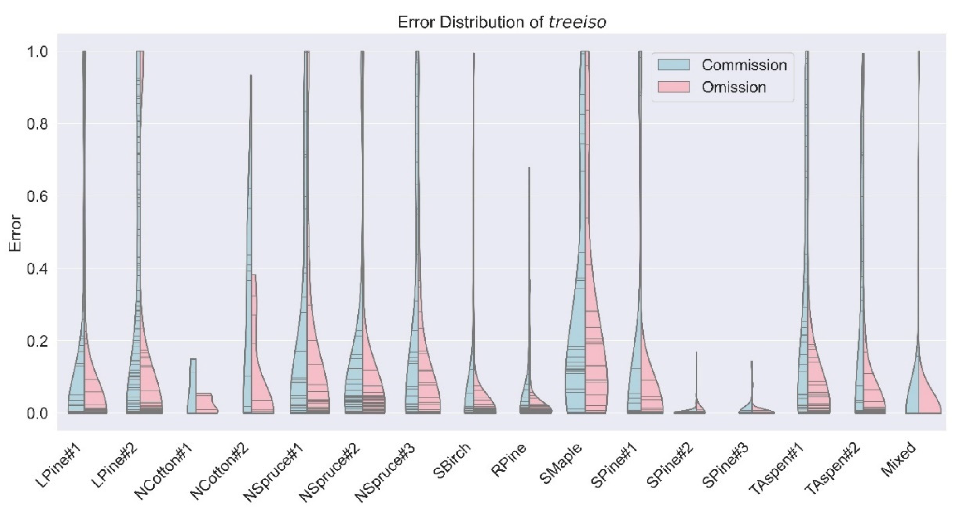
5.1. Distribution of Tree Isolation Error

Commission and omission errors of individual trees are summarized on a plot-wise basis using the violin charts in Figure 10. From most of the plots, omission error tended towards lower values than the commission error, as observed in the wider red violin distributions near the bottom. This effect occurred in both conifer and deciduous plots. It can be concluded, therefore, that the treeiso segmenter using the default parameter settings tended to slightly under-isolate trees. The average individual-tree commission error over all plots was 0.17, while the omission error was 0.08. NCotton#1, SPine#1, and SPine#2 successfully constrained both error types to below 0.2 among all trees due to the small sample size and comparatively simple isolation requirements. Both commission and omission errors extended to 1.0 among the larger and more complex plots, meaning certain reference trees were completely nonmatched or ignored. Both commission and omission errors were likely to occur among short trees. The average tree height was 15.4 m and 15.2 m among the trees with a high commission error (>0.9) and high omission error (>0.9), respectively, which was shorter than the 17.4 m mean height of all trees. Smaller trees were more susceptible to omission than commission. The average tree DBH with a high omission error (>0.9) was 17.1 cm, which was much smaller than the overall average of 27.0 cm, and also lower than the average DBH of 24.7 cm for trees with high commission error (>0.9). The omission problem of small trees, especially under the canopy of nearby tall trees, is also found by Hui et al. [59]. This indicates a need to improve treeiso (or to adjust default parameters) to better detect and isolate small trees.

5.2. Influence of Tree Attributes on Isolation Accuracy

Some plots with the same species have contrasting treeiso mIoU in Table 3, e.g., the two LPine plots and the two NCotton plots. Visually medium plots such as LPine#2 had lower accuracy than difficult level plots such as NSpruce plots. To explain the underlying causes of these IoU deviations from expectation, seven tree attributes were quantified for each tree and compared with the accuracy metrics using Pearson’s correlation r [60] (

Table 4. Pearson’s r between individual-tree attribute and accuracy metrics.

Attribute	IoU	Commission	Omission
N *	0.11	−0.11	−0.05
Height	0.18	−0.18	−0.06
DBH	0.02	−0.04	−0.03
Area	−0.01	−0.02	0.02
Overlap	−0.20	0.19	0.12
NNdist	0.18	−0.22	−0.08
Occlusion	0.10	−0.12	−0.07

* N is the total number of points from a tree.

). Area was defined as the area of the crown convex hull projected on the horizontal plane. Overlap was defined as the ratio of the horizontal crown area intersected by any neighbor crowns to the total horizontal area of the crown. NNdist was the nearest crown distance to the crown of interest. Occlusion was the ratio of the horizontal gap area within a crown to the total crown area. From Table 4, none of the seven factors had a strong correlation to the mIoU or errors. The maximum absolute value of r was 0.20, which suggests treeiso was not a simple model linear to a single geometric factor. There was, however, no obvious systematic weakness for isolating trees of variable geometries. Among the seven factors, Overlap, or crown overlap ratio, was most related to the tree isolation IoU (r = −0.20), and overlapped crowns could encounter greater commission error (r = 0.19). Strong overlap degree between crowns is a distinct factor contributing to large segmentation errors [35]. Tree height and NNdist were the other two factors demonstrating a small influence on the IoU and commission error. Taller trees with greater crown spacing are easier to isolate by treeiso. Occlusion (i.e., where a stem blocks other stems from the scanner field of view) demonstrated a low correlation (r = 0.10) with the IoU, which suggests that treeiso is at least somewhat able to mitigate the gaps and imperfect crown shapes that are often unavoidable in the operational scanning of dense tree plots. This is one advantage of treeiso relative to tree segmentation methods based on purely graph connectivity, such as Tao et al. [61].

Understanding the correlation between factors and accuracy helps explain why IoU deviates among the same species and apparent difficulty levels. The three most influential attributes, tree height, overlap, and NNdist, are illustrated with their average values for each plot in Figure 11. Tree height and NNdist were normalized to match the scale of the overlap attribute. Figure 11 clearly shows that NCotton#1 has a high NNdist, which contributed to its high mIoU of 0.91 compared to NCotton#2′s mIoU of 0.73 (see also Table 3). The highest mIoUs above 0.9 from RPine, SPine#2, SPine #3, and Mixed can all be explained by their low overlap ratio of <0.1. Figure 11 also confirms that the treeiso isolation accuracy was not a function of a single factor. For example, NCotton#1 and NCotton#2 shared a similar overlap ratio but their mIoUs varied greatly. RPine had a lower overlap ratio than SBirch, but its mIoU was greater by 0.06 due to its greater tree height and NNdist. LPine#2 was visually interpreted as having a medium isolation difficulty but its relatively high overlap ratio, short tree height, and small NNdist lead to a mIoU of 0.70, which is lower than some difficult deciduous plots such as NSpruce#1, TAspen#2, and NCotton#2.

6. Conclusions

In this study, a practical model treeiso based on the cut-pursuit graph algorithm was proposed to isolate individual-tree points from plot-level TLS scans. The treeiso followed the local-to-global segmentation scheme, which grouped points into small clusters, large segments, and final trees in a hierarchical manner. Using sixteen plots with manually isolated trees as reference, the isolation accuracy denoted by the mIoU was 0.82 on average, and the tree detection rate was 86%. Within the detected trees, the mIoU rose to 0.92. As a benchmark, the treeseg mIoU was 0.24, and the detection rate 67%. The tree geometry assumptions of treeseg, including the cylinder shape of the stem, predefined crown size, and simple connectivity rules, lead to many irregular tree components being ignored and an overall low accuracy. Individual-tree level commission and omission errors of treeiso were analyzed. The average commission error from all trees was 0.17, greater than the omission error of 0.08. Very small trees were found likely to cause high omission errors. Commission error was also more frequent among thinner and smaller trees. Seven tree attributes were investigated to understand the underlying determinants of isolation accuracy. No single attribute was significantly related to the treeiso accuracy. Three main attributes, crown overlap ratio, tree height, and NNdist, were jointly but weakly associated with the treeiso mIoU with Pearson’s r = −0.20, 0.18, 0.18, respectively. The three attributes successfully explain why mIoU varies greatly among plots with the same species or the same subjective difficulty level. It is also found that occlusion caused by crown mutual shadowing did not affect the treeiso accuracy greatly. A sensitivity analysis based on PAWN index was performed using a total of 10,000 parameter value combinations from the treeiso parameter space. Among the six tunable parameters of treeiso, three parameters $K_2$, ${\lambda }_2$, and $K_1$ were the key parameters influencing the tree isolation accuracy. The mIoU also changed slightly as the treeiso parameters varied. The processing time over sixteen plot scans was 2 h 16 min in total. Overall, the limited size of key tunable parameters, the robustness against parameter changes, and reasonable processing times render treeiso a useful and practical tool for plot-level TLS tree studies. The availability of baseline individual-tree data could eventually facilitate inventory data transfer from field measurements and physiological descriptors to broader models of landscape-scale ecosystem properties.

References

1. Blackard, J.A.; Finco, M.V.; Helmer, E.H.; Holden, G.R.; Hoppus, M.L.; Jacobs, D.M.; Lister, A.J.; Moisen, G.G.; Nelson, M.D.; Riemann, R.; et al. Mapping U.S. forest biomass using nationwide forest inventory data and moderate resolution information. Remote Sens. Environ. 2008, 112, 1658–1677. [Google Scholar] [CrossRef]
2. Beaudoin, A.; Bernier, P.; Villemaire, P.; Guindon, L.; Guo, X.J. Tracking forest attributes across Canada between 2001 and 2011 using ak nearest neighbors mapping approach applied to MODIS imagery. Can. J. For. Res. 2018, 48, 85–93. [Google Scholar] [CrossRef] [Green Version]
3. Zheng, J.; Fu, H.; Li, W.; Wu, W.; Yu, L.; Yuan, S.; Tao, W.Y.W.; Pang, T.K.; Kanniah, K.D. Growing status observation for oil palm trees using Unmanned Aerial Vehicle (UAV) images. ISPRS J. Photogramm. Remote Sens. 2021, 173, 95–121. [Google Scholar] [CrossRef]
4. Bouvier, M.; Durrieu, S.; Fournier, R.A.; Renaud, J.-P. Generalizing predictive models of forest inventory attributes using an area-based approach with airborne LiDAR data. Remote Sens. Environ. 2015, 156, 322–334. [Google Scholar] [CrossRef]
5. Hopkinson, C.; Chasmer, L.; Hall, R. The uncertainty in conifer plantation growth prediction from multi-temporal lidar datasets. Remote Sens. Environ. 2008, 112, 1168–1180. [Google Scholar] [CrossRef]
6. Popescu, S.C.; Wynne, R.H.; Nelson, R.F. Measuring individual tree crown diameter with lidar and assessing its influence on estimating forest volume and biomass. Can. J. Remote Sens. 2003, 29, 564–577. [Google Scholar] [CrossRef]
7. Coomes, D.A.; Dalponte, M.; Jucker, T.; Asner, G.P.; Banin, L.F.; Burslem, D.F.; Lewis, S.L.; Nilus, R.; Phillips, O.L.; Phua, M.-H. Area-based vs tree-centric approaches to mapping forest carbon in Southeast Asian forests from airborne laser scanning data. Remote Sens. Environ. 2017, 194, 77–88. [Google Scholar] [CrossRef] [Green Version]
8. Zianis, D.; Muukkonen, P.; Mäkipää, R.; Mencuccini, M. Biomass and Stem Volume Equations for Tree Species in Europe. Silva Fenn. Monogr. 2005, 4, 1–2. [Google Scholar] [CrossRef]
9. Hantsch, L.; Bien, S.; Radatz, S.; Braun, U.; Auge, H.; Bruelheide, H. Tree diversity and the role of non-host neighbour tree species in reducing fungal pathogen infestation. J. Ecol. 2014, 102, 1673–1687. [Google Scholar] [CrossRef] [Green Version]
10. Rozendaal, D.M.A.; Hurtado, V.H.; Poorter, L. Plasticity in leaf traits of 38 tropical tree species in response to light; relationships with light demand and adult stature. Funct. Ecol. 2006, 20, 207–216. [Google Scholar] [CrossRef]
11. Seidel, D.; Leuschner, C.; Müller, A.; Krause, B. Crown plasticity in mixed forests—Quantifying asymmetry as a measure of competition using terrestrial laser scanning. For. Ecol. Manag. 2011, 261, 2123–2132. [Google Scholar] [CrossRef]
12. Calders, K.; Newnham, G.; Burt, A.; Murphy, S.; Raumonen, P.; Herold, M.; Culvenor, D.S.; Avitabile, V.; Disney, M.; Armston, J.D.; et al. Nondestructive estimates of above-ground biomass using terrestrial laser scanning. Methods Ecol. Evol. 2015, 6, 198–208. [Google Scholar] [CrossRef]
13. Côté, J.-F.; Fournier, R.A.; Egli, R. An architectural model of trees to estimate forest structural attributes using terrestrial LiDAR. Environ. Model. Softw. 2011, 26, 761–777. [Google Scholar] [CrossRef]
14. Kankare, V.; Holopainen, M.; Vastaranta, M.; Puttonen, E.; Yu, X.; Hyyppä, J.; Vaaja, M.; Hyyppä, H.; Alho, P. Individual tree biomass estimation using terrestrial laser scanning. ISPRS J. Photogramm. Remote Sens. 2013, 75, 64–75. [Google Scholar] [CrossRef]
15. Hopkinson, C.; Chasmer, L.; Young-Pow, C.; Treitz, P. Assessing forest metrics with a ground-based scanning lidar. Can. J. For. Res. 2004, 34, 573–583. [Google Scholar] [CrossRef] [Green Version]
16. Chen, Y.; Zhang, W.; Hu, R.; Qi, J.; Shao, J.; Li, D.; Wan, P.; Qiao, C.; Shen, A.; Yan, G. Estimation of forest leaf area index using terrestrial laser scanning data and path length distribution model in open-canopy forests. Agric. For. Meteorol. 2018, 263, 323–333. [Google Scholar] [CrossRef]
17. Maas, H.-G.; Bienert, A.; Scheller, S.; Keane, E. Automatic forest inventory parameter determination from terrestrial laser scanner data. Int. J. Remote Sens. 2008, 29, 1579–1593. [Google Scholar] [CrossRef]
18. Greaves, H.E.; Vierling, L.A.; Eitel, J.U.H.; Boelman, N.T.; Magney, T.S.; Prager, C.M.; Griffin, K.L. Applying terrestrial lidar for evaluation and calibration of airborne lidar-derived shrub biomass estimates in Arctic tundra. Remote Sens. Lett. 2017, 8, 175–184. [Google Scholar] [CrossRef]
19. De Tanago, J.G.; Lau, A.; Bartholomeus, H.; Herold, M.; Avitabile, V.; Raumonen, P.; Martius, C.; Goodman, R.C.; Disney, M.; Manuri, S.; et al. Estimation of above-ground biomass of large tropical trees with terrestrial LiDAR. Methods Ecol. Evol. 2018, 9, 223–234. [Google Scholar] [CrossRef] [Green Version]
20. Liang, X.; Hyyppä, J.; Kaartinen, H.; Lehtomäki, M.; Pyörälä, J.; Pfeifer, N.; Holopainen, M.; Brolly, G.; Francesco, P.; Hackenberg, J.; et al. International benchmarking of terrestrial laser scanning approaches for forest inventories. ISPRS J. Photogramm. Remote Sens. 2018, 144, 137–179. [Google Scholar] [CrossRef]
21. Lin, Y.; Herold, M. Tree species classification based on explicit tree structure feature parameters derived from static terrestrial laser scanning data. Agric. For. Meteorol. 2016, 216, 105–114. [Google Scholar] [CrossRef]
22. Xi, Z.; Hopkinson, C.; Rood, S.B.; Peddle, D.R. See the forest and the trees: Effective machine and deep learning algorithms for wood filtering and tree species classification from terrestrial laser scanning. ISPRS J. Photogramm. Remote Sens. 2020, 168, 1–16. [Google Scholar] [CrossRef]
23. de Paula Pires, R.; Olofsson, K.; Persson, H.J.; Lindberg, E.; Holmgren, J. Individual tree detection and estimation of stem attributes with mobile laser scanning along boreal forest roads. ISPRS J. Photogramm. Remote Sens. 2022, 187, 211–224. [Google Scholar] [CrossRef]
24. Burt, A.; Disney, M.; Calders, K. Extracting individual trees from lidar point clouds using treeseg. Methods Ecol. Evol. 2019, 10, 438–445. [Google Scholar] [CrossRef] [Green Version]
25. Wang, J.; Chen, X.; Cao, L.; An, F.; Chen, B.; Xue, L.; Yun, T. Individual Rubber Tree Segmentation Based on Ground-Based LiDAR Data and Faster R-CNN of Deep Learning. Forests 2019, 10, 793. [Google Scholar] [CrossRef] [Green Version]
26. Raumonen, P.; Casella, E.; Calders, K.; Murphy, S.; Åkerblom, M.; Kaasalainen, M. Massive-scale tree modelling from TLS data. ISPRS Ann. Photogramm. Remote Sens. Spat. Inf. Sci. 2015, 2, 189. [Google Scholar] [CrossRef] [Green Version]
27. Liu, Q.; Ma, W.; Zhang, J.; Liu, Y.; Xu, D.; Wang, J. Point-cloud segmentation of individual trees in complex natural forest scenes based on a trunk-growth method. J. For. Res. 2021, 32, 2403–2414. [Google Scholar] [CrossRef]
28. Fu, H.; Li, H.; Dong, Y.; Xu, F.; Chen, F. Segmenting Individual Tree from TLS Point Clouds Using Improved DBSCAN. Forests 2022, 13, 566. [Google Scholar] [CrossRef]
29. Yang, B.; Dai, W.; Dong, Z.; Liu, Y. Automatic Forest Mapping at Individual Tree Levels from Terrestrial Laser Scanning Point Clouds with a Hierarchical Minimum Cut Method. Remote Sens. 2016, 8, 372. [Google Scholar] [CrossRef] [Green Version]
30. Heinzel, J.; Huber, M.O. Constrained Spectral Clustering of Individual Trees in Dense Forest Using Terrestrial Laser Scanning Data. Remote Sens. 2018, 10, 1056. [Google Scholar] [CrossRef]
31. Wang, D. Unsupervised semantic and instance segmentation of forest point clouds. ISPRS J. Photogramm. Remote Sens. 2020, 165, 86–97. [Google Scholar] [CrossRef]
32. Di Wang, D.; Liang, X.; Mofack, G.I.; Martin-Ducup, O. Individual tree extraction from terrestrial laser scanning data via graph pathing. For. Ecosyst. 2021, 8, 67. [Google Scholar] [CrossRef]
33. Fan, H.; Zhu, N.; Dong, Z. A Two-stage Approach for Individual Tree Segmentation from TLS Point Clouds. IEEE J. Sel. Top. Appl. Earth Obs. Remote Sens. 2022, 15, 8682–8693. [Google Scholar]
34. Redmon, J.; Farhadi, A. Yolov3: An incremental improvement. arXiv 2018, arXiv:1804.02767. [Google Scholar]
35. Zhong, L.; Cheng, L.; Xu, H.; Wu, Y.; Chen, Y.; Li, M. Segmentation of individual trees from TLS and MLS data. IEEE J. Sel. Top. Appl. Earth Obs. Remote Sens. 2016, 10, 774–787. [Google Scholar] [CrossRef]
36. Bellman, R. Dynamic programming. Science 1966, 153, 34–37. [Google Scholar] [CrossRef] [PubMed]
37. Frey, H.C.; Patil, S.R. Identification and Review of Sensitivity Analysis Methods. Risk Anal. 2002, 22, 553–578. [Google Scholar] [CrossRef]
38. Sobol, I.M. Sensitivity analysis for non-linear mathematical models. Math. Model. Comput. Exp. 1993, 1, 407–414. [Google Scholar]
39. Zadeh, F.K.; Nossent, J.; Sarrazin, F.; Pianosi, F.; van Griensven, A.; Wagener, T.; Bauwens, W. Comparison of variance-based and moment-independent global sensitivity analysis approaches by application to the SWAT model. Environ. Model. Softw. 2017, 91, 210–222. [Google Scholar] [CrossRef] [Green Version]
40. Borgonovo, E.; Castaings, W.; Tarantola, S. Moment Independent Importance Measures: New Results and Analytical Test Cases. Risk Anal. 2011, 31, 404–428. [Google Scholar] [CrossRef]
41. Pianosi, F.; Wagener, T. A simple and efficient method for global sensitivity analysis based on cumulative distribution functions. Environ. Model. Softw. 2015, 67, 1–11. [Google Scholar] [CrossRef] [Green Version]
42. Xi, Z.; Hopkinson, C. Detecting Individual-Tree Crown Regions from Terrestrial Laser Scans with an Anchor-Free Deep Learning Model. Can. J. Remote Sens. 2021, 47, 228–242. [Google Scholar] [CrossRef]
43. CloudCompare, 2.12 Beta. 2021. Available online: https://www.danielgm.net/cc/ (accessed on 6 May 2022).
44. Boykov, Y.; Kolmogorov, V. An experimental comparison of min-cut/max- flow algorithms for energy minimization in vision. IEEE Trans. Pattern Anal. Mach. Intell. 2004, 26, 1124–1137. [Google Scholar] [CrossRef] [PubMed]
45. Chambolle, A.; Darbon, J. On Total Variation Minimization and Surface Evolution Using Parametric Maximum Flows. Int. J. Comput. Vis. 2009, 84, 288–307. [Google Scholar] [CrossRef] [Green Version]
46. Boykov, Y.Y.; Jolly, M.-P. Interactive graph cuts for optimal boundary & region segmentation of objects in N-D images. In Proceedings of the Eighth IEEE International Conference on Computer Vision ICCV 2001, Vancouver, BC, Canada, 7–14 July 2001; pp. 105–112. [Google Scholar]
47. Landrieu, L.; Obozinski, G. Cut Pursuit: Fast Algorithms to Learn Piecewise Constant Functions on General Weighted Graphs. SIAM J. Imaging Sci. 2017, 10, 1724–1766. [Google Scholar] [CrossRef] [Green Version]
48. Raguet, H.; Landrieu, L. Cut-pursuit algorithm for regularizing nonsmooth functionals with graph total variation. In Proceedings of the International Conference on Machine Learning, Stockholm, Sweden, 10–15 July 2018; Volume 80, pp. 4247–4256. [Google Scholar]
49. Bechtel, B.; Ringeler, A.; Böhner, J. Segmentation for Object Extraction of Trees using MATLAB and SAGA. SAGA–Second. Out, Hambg. Beitr. Zur Phys. Geogr. Landschaftsökologie. Univ. Hambg. Inst. Geogr. 2008, 19, 1–12. [Google Scholar]
50. Xi, Z.; Hopkinson, C.; Chasmer, L. Filtering Stems and Branches from Terrestrial Laser Scanning Point Clouds Using Deep 3-D Fully Convolutional Networks. Remote Sens. 2018, 10, 1215. [Google Scholar] [CrossRef] [Green Version]
51. Kisantal, M.; Wojna, Z.; Murawski, J.; Naruniec, J.; Cho, K. Augmentation for small object detection. arXiv 2019, arXiv:1902.07296. [Google Scholar]
52. Schubert, M.; Kahl, K.; Rottmann, M. MetaDetect: Uncertainty Quantification and Prediction Quality Estimates for Object Detection. In Proceedings of the 2021 International Joint Conference on Neural Networks (IJCNN), Shenzhen, China, 18–22 July 2021; pp. 1–10. [Google Scholar] [CrossRef]
53. Brede, B.; Calders, K.; Lau, A.; Raumonen, P.; Bartholomeus, H.M.; Herold, M.; Kooistra, L. Non-destructive tree volume estimation through quantitative structure modelling: Comparing UAV laser scanning with terrestrial LIDAR. Remote Sens. Environ. 2019, 233, 111355. [Google Scholar] [CrossRef]
54. Stovall, A.E.; Anderson-Teixeira, K.J.; Shugart, H.H. Assessing terrestrial laser scanning for developing non-destructive biomass allometry. For. Ecol. Manag. 2018, 427, 217–229. [Google Scholar] [CrossRef]
55. MATLAB 2020b; The MathWorks Inc.: Natick, MA, USA, 2020.
56. Herman, J.; Usher, W. SALib: An open-source Python library for Sensitivity Analysis. J. Open Source Softw. 2017, 2, 97. [Google Scholar] [CrossRef]
57. Seaholm, S.K.; Ackerman, E.; Wu, S.-C. Latin hypercube sampling and the sensitivity analysis of a Monte Carlo epidemic model. Int. J. Bio-Medical Comput. 1988, 23, 97–112. [Google Scholar] [CrossRef] [PubMed]
58. Puy, A.; Piano, S.L.; Saltelli, A. A sensitivity analysis of the PAWN sensitivity index. Environ. Model. Softw. 2020, 127, 104679. [Google Scholar] [CrossRef]
59. Hui, Z.; Jin, S.; Li, D.; Ziggah, Y.Y.; Liu, B. Individual Tree Extraction from Terrestrial LiDAR Point Clouds Based on Transfer Learning and Gaussian Mixture Model Separation. Remote Sens. 2021, 13, 223. [Google Scholar] [CrossRef]
60. Benesty, J.; Chen, J.; Huang, Y.; Cohen, I. Pearson correlation coefficient. In Noise Reduction in Speech Processing; Springer: Berlin/Heidelberg, Germany, 2009; Volume 2, pp. 1–4. [Google Scholar] [CrossRef]
61. Tao, S.; Wu, F.; Guo, Q.; Wang, Y.; Li, W.; Xue, B.; Hu, X.; Li, P.; Tian, D.; Li, C.; et al. Segmenting tree crowns from terrestrial and mobile LiDAR data by exploring ecological theories. ISPRS J. Photogramm. Remote Sens. 2015, 110, 66–76. [Google Scholar] [CrossRef]
Figure 1. Geolocations of nine Canadian sites with TLS scan collection. Ecozone names are italic. Green dots indicate plot locations and nearby labels show plot ID names.
Remotesensing 14 06116 g001
Figure 2. Manually isolated point clouds from sixteen TLS plot scans. Each individual tree was assigned a random color to help visual identification. Geolocations of eight Canadian sites with TLS scan collection. Ecozone names are Italic.
Remotesensing 14 06116 g002
Figure 3. treeiso’s workflow.
Remotesensing 14 06116 g003
Figure 4. Iteratively cutting a point cloud graph into meaningful clusters using the 0 cut pursuit algorithm. The point cloud graph is composed of nodes (numbered) and edges (lines between nodes).
Remotesensing 14 06116 g004
Figure 5. Geometrical illustration of calculating elevation-difference-to-length ratio (a) and the nearest measure between segments (b).
Remotesensing 14 06116 g005
Figure 6. Intermediate output of treeseg and treeiso algorithms with three TAspen#1 tree point clouds as an example: (a) initial stem finding (in brown), and full-grown isolated stem (in red, green and blue, respectively) from treeseg; (b) result isolated trees from treeseg; (c) manually isolated reference trees; (d) initial clusters from first-stage segmentation of treeiso; (e) merged segments from the second-stage segmentation of treeiso; (f) result isolated trees from treeiso after global connection; (g) result treeseg trees from top view; (h) result treeiso trees from top view; and (i) reference trees from top view. Different clusters or segments are colored randomly. The average of the three tree heights is 12.8 m.
Remotesensing 14 06116 g006aRemotesensing 14 06116 g006b
Figure 7. Example plot tree isolation from treeiso compared with reference: Spine#1 treeiso (a) and reference (d), LPine#1 treeiso (b) and reference (e), TAspen#1 treeiso (c) and reference (f) from top view, and TAspen#1 treeiso (g) and reference (h) from side view. The plot orientations are the same between treeiso results and references. Different individual trees are assigned different colors randomly. The random colors can help identify individual trees but might distract the visual comparison between the treeiso results and references. Tree shapes and locations, instead of colors, are suggested for the tree-wise visual comparison under this circumstance.
Remotesensing 14 06116 g007
Figure 8. Parameter sensitivity analysis using the PAWN index.
Remotesensing 14 06116 g008
Figure 9. Summary of accuracy response conditional to separate parameter variation based on the 10,000 samples. All parameters were scaled between 0–1 based on the ranges in Table 2. The lines connect the means of the mIoU distributions within each interval, and the band around each line illustrates the 95% confidence interval.
Remotesensing 14 06116 g009
Figure 10. Plot-level summaries of the commission and omission error distributions for individual trees. The commission and omission error were placed side by side for each of the sixteen plots to provide visual contrast. Within each violin, each tree has one commission (one solid horizontal line in the light blue half) and one omission error (one solid horizontal line in the light pink half). A violin creates a smooth outline to illustrate the distribution of plot-level error frequencies. The width of one horizontal line denotes the relative frequency of the error where the total area of a violin is normalized to 1.
Remotesensing 14 06116 g010
Figure 11. Tree attributes averaged over each plot. Height is divided by 30 m and NNdist divided by 6 m to reduce the bar height difference from Overlap for better visualization.
Remotesensing 14 06116 g011