Article

Exploring the Spatio-Temporal Characteristics of Urban Thermal Environment during Hot Summer Days: A Case Study of Wuhan, China

College of Resources and Environment, Huazhong Agricultural University, Wuhan 430070, China
*
Author to whom correspondence should be addressed.
Remote Sens. 2022, 14(23), 6084; https://doi.org/10.3390/rs14236084
Submission received: 31 October 2022 / Revised: 24 November 2022 / Accepted: 26 November 2022 / Published: 30 November 2022
(This article belongs to the Special Issue Geographical Analysis and Modeling of Urban Heat Island Formation)

Abstract

:
An urban thermal environment is an area receiving special attention. In order to effectively explore its spatio-temporal characteristics during hot summer days, this study introduced the standard deviational ellipse (SDE) to construct an urban heat island index to describe the general spatial character of an urban thermal environment, and then used local Moran’s I to identify its local spatial cluster characteristics. Finally, the regressions of ordinary least squares (OLS) and spatial lag model (SLM) were adopted to explore the effect of woodland, water body and impervious surface on the thermal environment. Taking the city of Wuhan as a study area and using the air temperature on seven consecutive days, from 17 July to 23 July in 2018, from the China Meteorological Administration Land Data Assimilation System (CLDAS-V2.0), the results show that the urban heat island index can effectively represent the general characteristics of the thermal environment. The general trends of heat island intensity decrease first and then increase from 00:00 to 24:00. The heat island intensity is at its minimum from 10:00 to 16:00, and at its maximum from 22:00 to 4:00 the next day. Local Moran’s I values indicate that the clusters of high air temperature at 06:00 and at 22:00 are associated with the impervious surface and the water body. This is further illustrated by the regression analysis of OLS, which can explain 50–60% of the spatial variation of the air temperature. Then, the fitness of the SLM is greatly improved; the coefficients of determination at 06:00 and at 22:00 are all not less than 0.97. However, the explanation of the local land uses accounting for the spatial variation of the air temperature becomes lower. The regression analysis also shows that the woodland always has the effect of decreasing air temperature at 06:00, 14:00 and 22:00, implying that increasing the vegetation may be the most effective way to mitigate the adverse circumstance of the urban thermal environment.

1. Introduction

Human activities, especially urbanization, have gradually changed the Earth’s surface landforms, and then caused changes in the urban thermal environments. Urban heat island (UHI) effect, a phenomenon according to which urban areas have higher air temperatures than the surrounding rural areas, is a prominent problem of the urban thermal environment. The effect of UHI on heat wave intensifies during the period of prolonged extreme heat [1], and the synergy [2] between the two even causes an increased heat stress that is higher than the combined effect of the background UHI and heat waves [3], which may increase the mortality related to high temperatures in urban areas [4] and have a profound impact on the human living environments [5].
Land cover change through urban sprawl and cultivated land degradation has a dramatic effect on UHI intensity [6], as the city with a higher urban land cover usually has the higher UHI intensity [7]. Moreover, the urban radiant heat is varied and depends largely on the type of land cover and urban surface [8]. Different land uses have different effects on UHI [9]. The lack of vegetation may contribute to higher temperatures in industrial parks, while the temperatures go up by up to 2 °C in commercial districts on weekends [10]. It is found that the impervious surface area (ISA) is the most significant factor causing the increasing temperature [11], while the land surface temperature (LST) generally increases in parallel with the ISA [12]. Then, the urban green space and its spatial configurations, such as larger patches, simpler shapes, being more connected and less fragmented, have a significant effect on the LST [13]; in particular, they contribute to a lower LST [14,15].
Effective water resources management is also of great significance to reduce the heat island effect [16]. Studies have found that the intensity of the UHI effect decreases by 11.33% with the increase in water-body coverage by 10% during the daytime [17]. However, the water will increase the UHI effect after the evening, for its high heat capacity inhibits its circulation and makes it remain at relatively high temperatures [18].
There are many types of UHIs [19], of which the most commonly used are surface UHI (SUHI), based on LST, and canopy UHI (CUHI), based on air temperature within the urban canopy layer. These two types of UHI depict the thermal environment characteristics in different vertical layers of the urban structure. The approaches to measure the two types of UHI both have advantages and disadvantages [20]. Most of the studies focus on SUHIs because the LST data are easy to obtain from remote sensing, but the uncertainty of the LST is too great to obtain reliable urban thermal trends [21]. Moreover, the CUHIs described by using air temperature, which is obtained through meteorological field measurements, is more relevant to public health [22] and is a key parameter for studying the UHI effect [23].
Although there are a large number of studies focusing on UHI, some problems with respect to it are still ambiguous. The UHI intensity is conventionally defined as the difference in temperature between an urban and rural area [24]. The traditional detection of intensity is conducted at two fixed in situ stations in urban and rural regions [25]. Similarly, the calculation of the surface UHI is conducted over selected pixels located in the urban and rural regions based on remote sensing data [26]. The estimations both depend on the determination of urban and rural stations or pixels [23,27]. However, the air temperatures of the urban area are heterogeneous in space, and the choice of a rural area also affects the quantification. There are some modified methods to improve the estimation [28,29,30,31,32], such as calculating the average temperature of the corresponding areas, but the spatial characteristics of the urban thermal environment are still not good enough to present. In addition, the studies on the evolution of the spatio-temporal characteristics of the urban thermal environment during a day are scarce.
Thus, this study focuses on the air temperature and introduces the standard deviational ellipse (SDE) to explore the general spatial distribution of an urban thermal environment. We then further construct an UHI index to characterize UHI intensity. This index is not just determined by the air temperatures of two points but with the purpose of effectively reflecting the general spatial character of the urban thermal environment. Taking the city of Wuhan as a study area, and using the air temperature data of seven consecutive days with sunny and cloudy weather conditions in the hot summer of 2018, we first analyzed the general spatial thermal character and calculated the UHI index every two hours during the seven days. Then, we chose three time points in each day and used local Moran’s I to explore the local spatial pattern of the thermal environment in the study area. Furthermore, the regression analysis including ordinary least squares (OLS) and the spatial lag model (SLM) are adopted to explore the land uses that contribute to the spatial variation of air temperature. The efforts of this work are aimed at trying to provide a method to characterize the spatial distribution of the thermal environment and the UHI effect more effectively as well as to illustrate their evolutions with the high temporal resolution during a day.

2. Materials and Methods

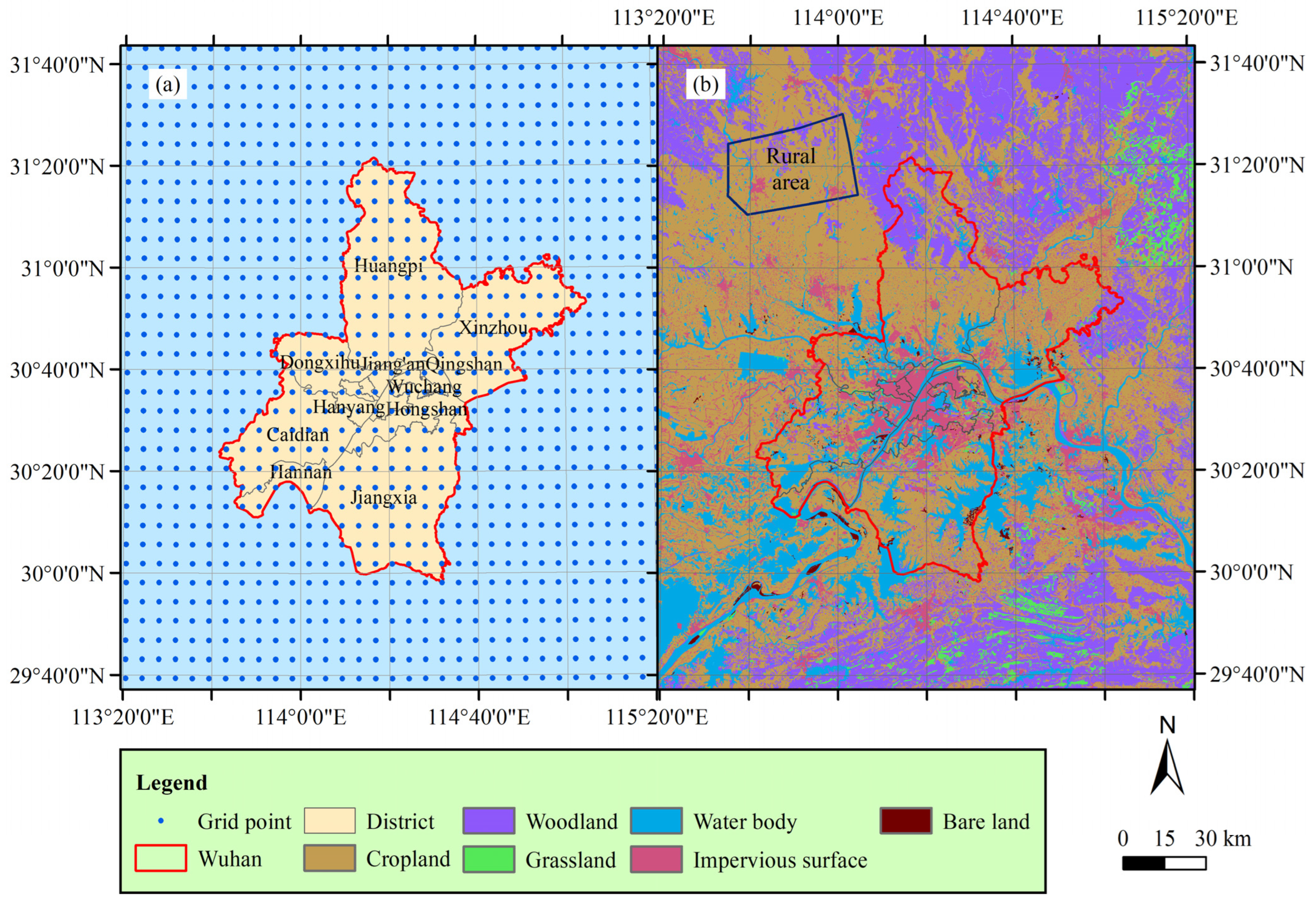
2.1. Study Area and Data Source

Wuhan, the capital of Hubei Province, is the city with the largest population in Central China, between the latitudes 29°58′19.04″N and 31°21′44.07″N and between the longitudes 113°41′32.86″E and 115°4′55.70″E, covering a total area of approximately 8624.69 km2 (Figure 1a), and with an average elevation of about 37 m above sea level. The city possesses the distinctive character of having a large number of water bodies (Figure 1b), which is why it was once called “the city of a thousand lakes”. According to Köppen climate classification, the study area has a Cfa climate with abundant rainfall, cool winters and hot summers. As one of the Four Furnaces of China, Wuhan is always suffering heat waves and high air temperatures in the summertime.
In this study, we focused on the days that are the hottest in the summer. Additionally, both sunny and cloudy days are included in our analysis to compare the differences in thermal environmental characteristics between the two weather conditions. Thus, we chose the days from 17 July to 23 July in 2018 as the study period. The weather of the middle three days in the study area was sunny, while for the four other days it was cloudy, which is illustrated in Table 1. The air temperature (2 m above the land surface) of these seven days was obtained from the China Meteorological Administration (CMA) Land Data Assimilation System (CLDAS) version 2.0 dataset, called “CLDAS-V2.0” dataset, in China Meteorological Data Service Centre. The “CLDAS-V2.0” dataset is a grid fusion analysis dataset with the resolution of 0.0625° × 0.0625° and 1 h. There are 207 grid points in the city of Wuhan; the distance between two adjacent grid points in the east–west direction is about 6.0 km and that in the north–south direction is about 6.9 km (Figure 1a). The dataset is developed by using a multiple-grid variational assimilation called Space and Time Mesoscale Analysis System (STMAS), along with physical inversion, terrain correction based on the ground, satellite observations from various sources and CLM3.5, CoLM, Noah-MP land surface model. Evaluated by 2400 in situ national automatic stations of the China Meteorological Administration (CMA), the RMSE of the 2 m air temperature of the dataset is 0.88 °C; the bias is −0.13 °C; and the correlation coefficient is 0.97 (http://data.cma.cn/en/?r=data/detail&dataCode=NAFP_CLDAS2.0_NRT, accessed on 16 November 2020). Studies evaluating the near-surface air temperature of CLDAS also show that it has a high reliability in China and is significantly correlated with the observations [33,34]. The dataset has been widely used in various studies [35,36,37,38].
The land use data of the study area are from Resource and Environment Science and Data Center, Chinese Academy of Sciences (https://www.resdc.cn, accessed on 17 October 2021). The data include 6 major categories of cropland, woodland, water body, impervious surface and bare land as well as 25 secondary classes, with a resolution of 30 m by 30 m (Figure 1b). The overall accuracy of the data is about 95% for 25 secondary land use classes [39].

2.2. Standard Deviational Ellipse and Urban Heat Island Index

The standard deviational ellipse (SDE) is a technique to explore spatial distributions. It was first introduced in study of geographic density in sociology, such as population distribution [40], and is now widely used to estimate spatial distribution evolutions and trends [41,42]. We employed this technique in this study. Moreover, we further developed a new index based on it.
The analysis of the SDE includes weighted SDE and non-weighted SDE. The steps of calculating the weighted SDE are as follows. The first is to calculate the weighted mean center of the point set, which is given by:
x ¯ w = i = 1 n w i x i i = 1 n w i , y ¯ w = i = 1 n w i y i i = 1 n w i ,
where xi and yi are the coordinates of the ith point; n is the total number of the points; wi is the weight of the ith point. Thereafter, the transformed coordinates, which are the different metric spaces between the ith point and the weighted mean center, are given as follows:
x i = x i x ¯ w , y i = y i y ¯ w .
Then, the angle of rotation, measured clockwise from North to the long axis of the ellipse, can be calculated by:
tan θ = i = 1 n w i 2 x i 2 i = 1 n w i 2 y i 2 + i = 1 n w i 2 x i 2 i = 1 n w i 2 y i 2 2 + 4 i = 1 n w i 2 x i y i 2 2 i = 1 n w i 2 x i y i .
Finally, the standard distances of the ellipse on x and y directions can be produced by:
σ x = i = 1 n w i x i cos θ w i y i cos θ 2 i = 1 n w i 2 ,
σ y = i = 1 n w i x i cos θ + w i y i cos θ 2 i = 1 n w i 2 .
When wi = 1 in the above equations, the results of the weighted SDE are the same as the non-weighted SDE. In this study, we use the weighted SDE to explore the spatial distribution of air temperature and combine its results with those of the non-weighted SDE for further analysis. Evidently, the weight of a point relates to the air’s temperature. However, if the weight is set equal to the air temperature of the point, the weight discrimination is very small for the minor difference between the air temperature of the maximum and the minimum in the study area, which is about 5 °C or even less, whereas the air temperature of the point is generally around 30 °C. Therefore, we introduce the air temperature of an area identified as rural and use it combined with the air temperature of the grid point to construct the weight. Since the weight cannot be negative, the functional form of the weight is constructed as:
w i = f T a i , T a r = exp T a i T a r ,
where Tai is the air temperature (°C) of the ith point and Tar indicates the air temperature (°C) of the rural area. Therefore, what an area is considered as rural, distinguished from the urban area, is a key point. We first analyzed the air temperature isotherm and the air temperature profile of an extended area covering the city of Wuhan. Then, based on combined analysis of air temperature distribution and land use configuration, we identified a typical area as rural. Thereafter, we calculated the mean value of the air temperature with respect to the grid points in the typical rural area and used this mean value as the Tar. Since a higher wi is obtained with a higher Tai, it is evident that the higher the Tai near the center of the study area, the smaller the standard distances of the ellipse in Equations (4) and (5). This suggests that the smaller the area of the weighted SDE, the more intensive the heat island effect. As for the non-weighted SDE, it is equivalent to considering all the grid points to have equal weights; that is to say, all the grid points with the same air temperature, representing the state of having no heat island effect in the study area. Therefore, we construct an UHI index that reflect the heat island intensity, as follows:
I = S S D E n o n W S S D E W = π σ x n o n W σ y n o n W π σ x W σ y W = σ x n o n W σ y n o n W σ x W σ y W ,
where SSDE−nonW, σx−nonW and σy−nonW are the area and standard deviations on x and y directions of the non-weighted SDE, respectively; SSDE−W, σx−W and σy−W are those of the weighted SDE. When the value of this index is larger than 1, this indicates that the corresponding area presents the state of the heat island effect. Moreover, the weaker the heat island effect of the study area, the closer the value of this index is to 1, and the more intensive the heat island effect, the larger the value of the index. Conversely, a value of the UHI index less than 1 suggests that the weights of the grid points near the center are lesser than those far from the center. Since the wi monotonically increases with the Tai base on Equation (6), the air temperature has the same spatial distribution trend as the weights, therefore representing the state of cool island.

2.3. Spatial Pattern Analysis

Spatial autocorrelation refers to the potential interdependence of observed data of some variables within the same distribution area. Moran’s I is a commonly used spatial autocorrelation statistic to describe the concentration or dispersion of variables in space. Moran’s I can be divided into global Moran’s I and local Moran’s I. Global Moran’s I shows whether there exists aggregation or outliers in a space, and is then used for exploring the global correlation between regions. The local Moran’s I [43], a statistic to measure the local spatial autocorrelation index, is used to reflect the characteristics of agglomeration and differentiation of related variables in a small-scale spatial structure, which is used in this study to analyze the spatial pattern of the air temperature of the study area. It can be expressed as follows:
I i = Z i W Z i ,
where
Z i = T a i T a ¯ S ,
W Z i = j = 1 , j i n w i j * Z j = j = 1 , j i n w i j * T a j T a ¯ S ,
where Tai is the air temperature of grid point I; T a ¯ and S are the mean and the standard deviation of the air temperatures of all grid points in the study area, respectively; n is the total number of the grid points; and wij* is a normalized spatial weight of point j with respect to point i, derived from a non-normalized spatial weight. In this study, the non-normalized spatial weight is defined as the inverse of the distance squared, which is given by:
w i j = 1 / d i j 2 , d i j b 0 , d i j > b ,
where dij is the distance between grid point i and j; b is a distance bandwidth. In this study, b is specified with the value of 11 km, which implies that only the grid points surrounding the grid point i have weights larger than 0, with other grid points given the weights of 0. Usually, there are 8 points surrounding a grid point, but less than 8 points for each of the points at the edge of the study area. Thereafter, the normalized spatial weight is given by:
w i j * = w i j / j = 1 , j i n w i j .
In Equations (8)–(10), Zi describes the air temperature of point i in deviations from the mean of air temperature of the study area and WZi represents the weighted summation of air temperature deviations of the grid points surrounding point i from the mean of air temperature. Through the analysis of local Moran’s I, the patterns of spatial clusters of grid points and the outliers with a statistically significance can be obtained. If Zi > 0 and WZi > 0, this means the grid point and the outliers have high values (relative to the mean value), called the cluster of high values (HH). If Zi < 0 and WZi < 0, this means the grid point and the outliers have low values (relative to the mean value), called the cluster of low values (LL). The other two patterns are the grid point having a high value and surrounded by grid points with low values (HL), with Zi > 0 and WZi < 0, and the grid point having a low value and surrounded by grid points with high values (LH), with Zi < 0 and WZi > 0.

2.4. Regression Analysis

Linear regression analysis is a common method to analyze the relationship of a dependent variable driven by other factors. In this study, the dependent variable is the air temperature of the grid point, and the independent variables are the proportions of the land uses in the area with respect to the Thiessen polygon of each grid point. The ordinary least squares (OLS) model, involving a global multiple linear regression (MLR) in this study, is formed as:
T a = X β + ε ,
where Ta is a vector with respect to the air temperature of the grid points of the study area; X is a matrix containing intercept (a vector of ones with the length equal to the total number of the grid points) and values of land use fractions of the Thiessen polygon corresponding to each grid point; β is a vector of the regression coefficients; and ε is a vector of random errors. Additionally, stepwise regression technology is used to select the proper explanatory variables from the proportions of the six land use types illustrated in Figure 1b.
Usually, there are spatial autocorrelations with geographical variables. Thus, spatial regression models may be more effective in explaining the relationship of the variables compared with the OLS model. Spatial lag model (SLM) and spatial error model (SEM) are two common types of spatial regression model [44]. Since SLM is mostly suitable to deal with the problem associated with spatial diffusion, a characteristic of heat, we adopt SLM to further analyze air temperature with driving factors. The SLM adds an autocorrelation term of the air temperature of the grid points to the right of Equation (13). Additionally, the driving factors that we use for the model are the final selected explanatory variables based on the stepwise regression analysis. The model is described as follows:
T a = ρ W T a + X β + ε ,
where ρ is the parameter characterizing the contribution of spatial autocorrelation; W is a row-sum standardized spatial weight matrix with the elements of wii* = 0 and wij* calculated by Equation (12); and WTa represents the spatially lagged response of the air temperature of the grid points.

3. Results

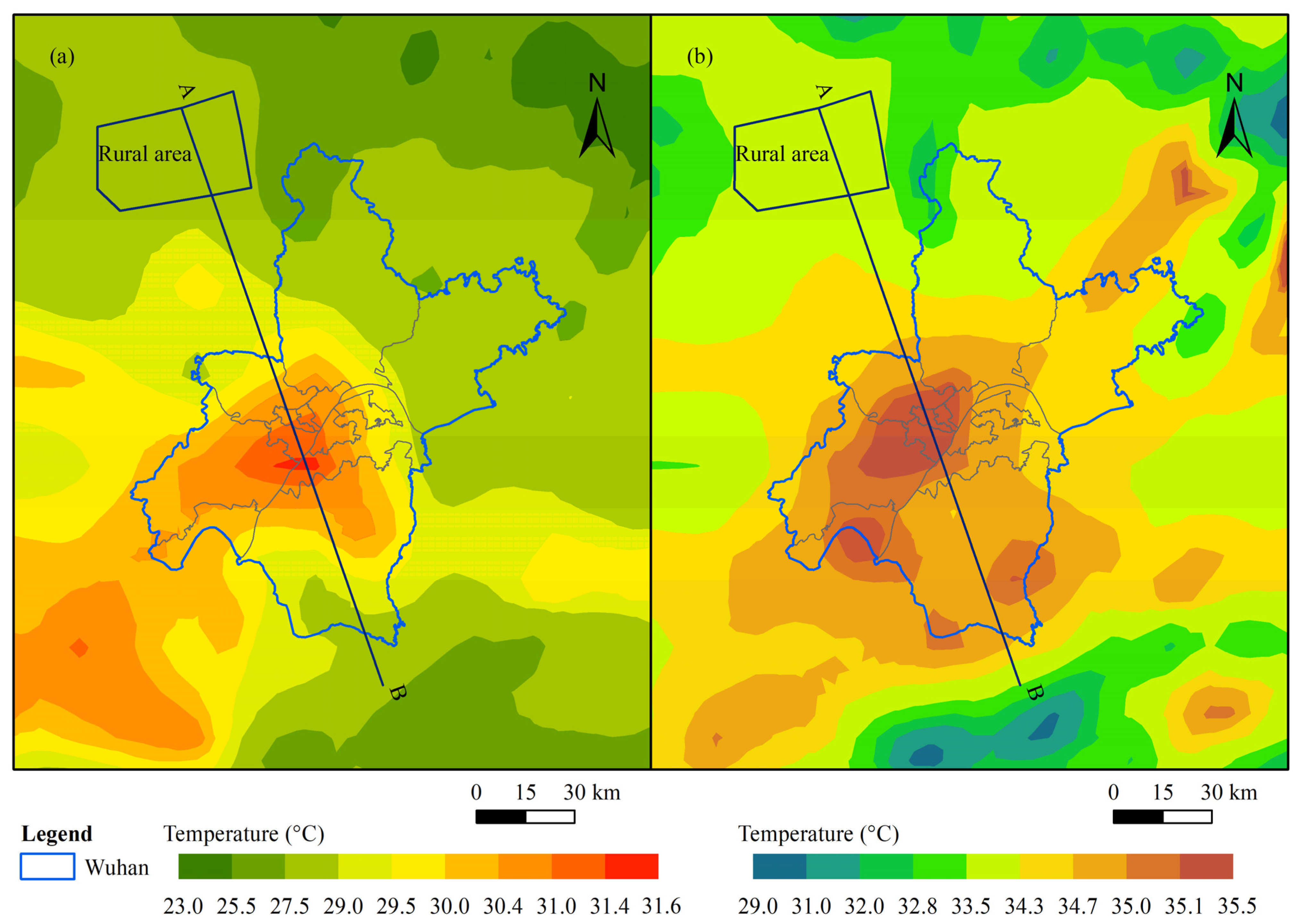
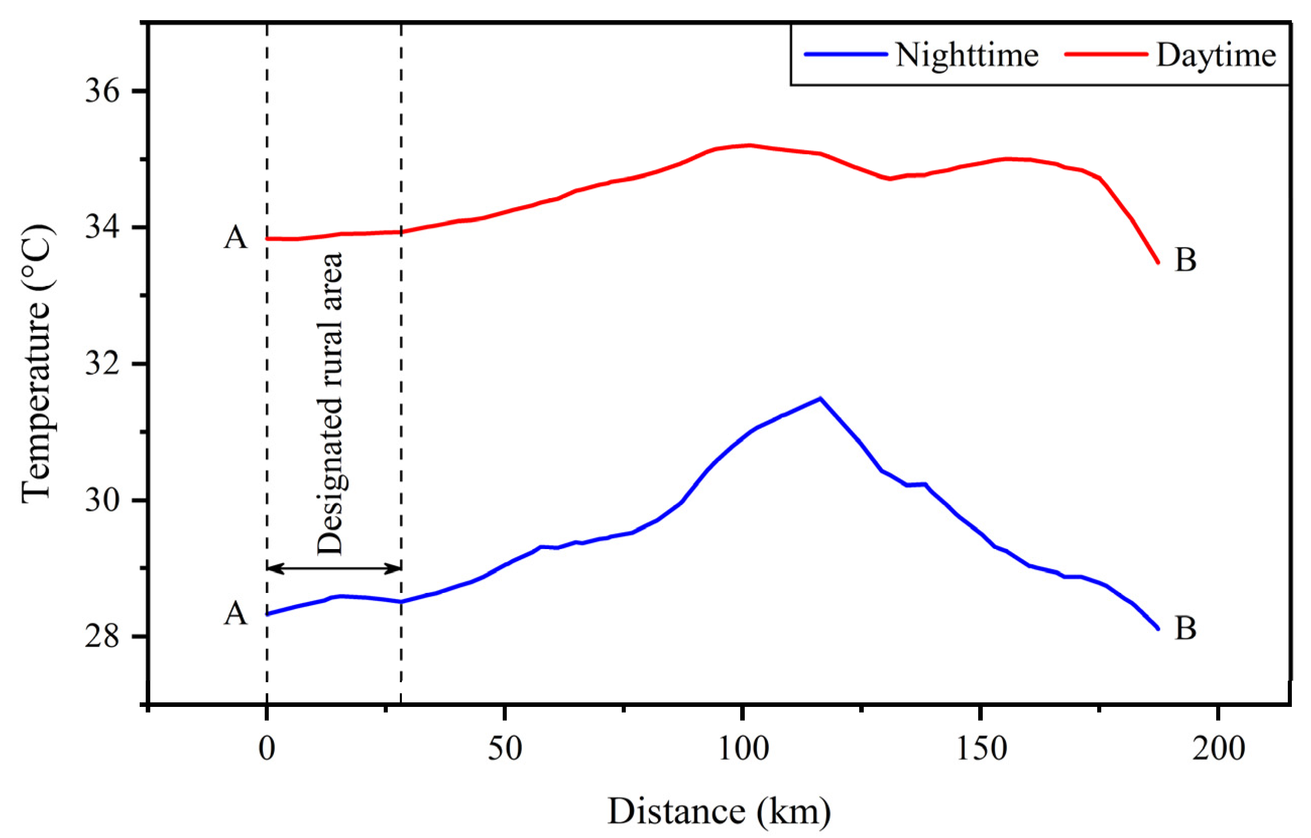
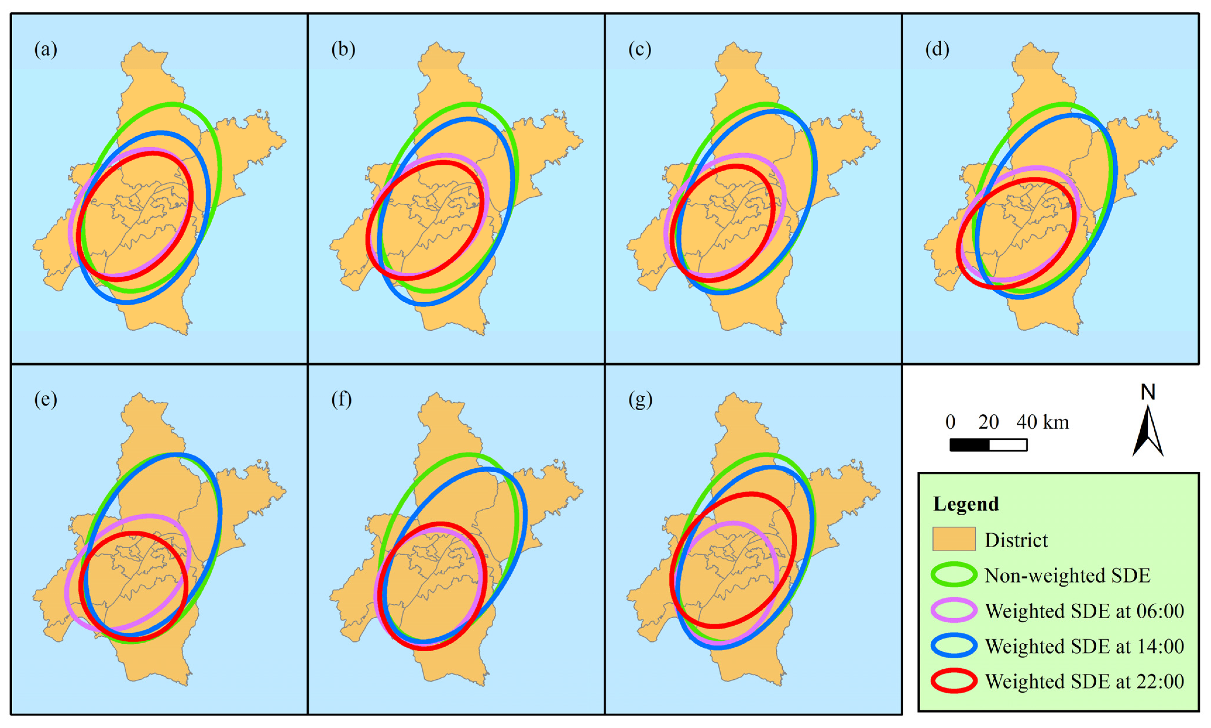
3.1. General Spatio-Temporal Distribution of the Thermal Environment

We calculated the mean air temperature of the grid points in an extended area including the city of Wuhan during the nighttime (20:31 the day before to 06:30) and the daytime (06:31 to 20:30) from 17 July to 23 July. We then plotted the air temperature isotherms, which are illustrated in Figure 2. It can be seen that the islands of air temperature protrude above the surrounding air temperature field both during nighttime and daytime, revealing that heat islands are present in the city of Wuhan. The center of the heat island is slightly southwest of the city center during the nighttime, and slightly west of the city center during the daytime. The northern region is relatively cool compared to the entire city. Furthermore, we analyzed the air temperature profile along the line of AB in Figure 2. The profiles of the air temperature are shown in Figure 3. Based on the combined analysis of air temperature distribution and land use configuration, we chose a typical rural area located to the northwest of the city of Wuhan, illustrated in Figure 2. The air temperature of the designated rural area is flat, which means that the change rate is small, as seen from the profiles (Figure 3), and the air temperature gradient on the designated rural area boundary toward the city center is uphill and increased. On the other hand, as seen in Figure 1b, the designated rural area is dominated by the cropland and contains some woodland and a small amount of impervious surface. All these temperature and land use characteristics are typical of rural areas. Therefore, we used the mean air temperature of the grid points in this area to represent the rural air temperature.
After determining the rural air temperature, the weights of the grid points were obtained according to Equation (6). Then, we took the 207 grid points in the city of Wuhan for the SDE analysis. Furthermore, based on Equation (7), the values of the UHI index for every two hours from 00:00 on 17 July to 00:00 on 24 July were derived, which are shown in Figure 4. The trends of the UHI index within each day are very similar, generally decreasing from 04:00 to 10:00 and increasing from 16:00 to 22:00. The UHI index minimum of each day occurs between 10:00 and 16:00, and the maximum occurs between 22:00 and 04:00 the next day. Additionally, the difference between the UHI index minimum of these seven days is very small. However, the peak values of the UHI index curve from the evening of 19 July to the early morning of 22 July are obviously higher than those of the other days. The weather from 19 July to 21 July is sunny, while the other days it is cloudy, which indicates that sunny days enhance the heat island effect at night compared to cloudy days, but the heat island effect with respect to the two weather conditions during the day is not much different.
The non-weighted SDEs and the weighted SDEs at 06:00, 14:00 and 22:00 of the seven days are illustrated in Figure 5. The center of the non-weighted SDEs represents the geographical center of the study area, and that of the weighted SDEs represents the center of the thermal field. It is evident that the centers of the thermal fields in the morning and at night are southwest of the geographical center of the city. Moreover, the shape of the weighted SDEs can reflect the dispersion of air temperature. Similar to the spatially normal distribution, the ellipse of the one standard deviation encompasses approximately 68% of the cumulate air temperature weights (wi in Equation (6)) in the area. Except for 21 and 23 July, the weighted SDEs at 06:00 and 22:00 each day are close in shape, position and size. This illustrates that the spatial distributions of the thermal characteristics at 06:00 and at 22:00 are very similar. Likewise, the weighted SDE at 14:00 and the non-weighted SDEs are close in shape, position and size except for 17 and 22 July. Since the non-weighted SDE is considered as having no heat island effect, the results illustrate that the heat islands at 14:00 are weak. On the contrary, as shown in Figure 5, the distinction of the weighted SDEs at 06:00 and at 22:00 from the non-weighted SDEs are broad, especially in size and position, indicating that the heat island effect is intense at these two time points.

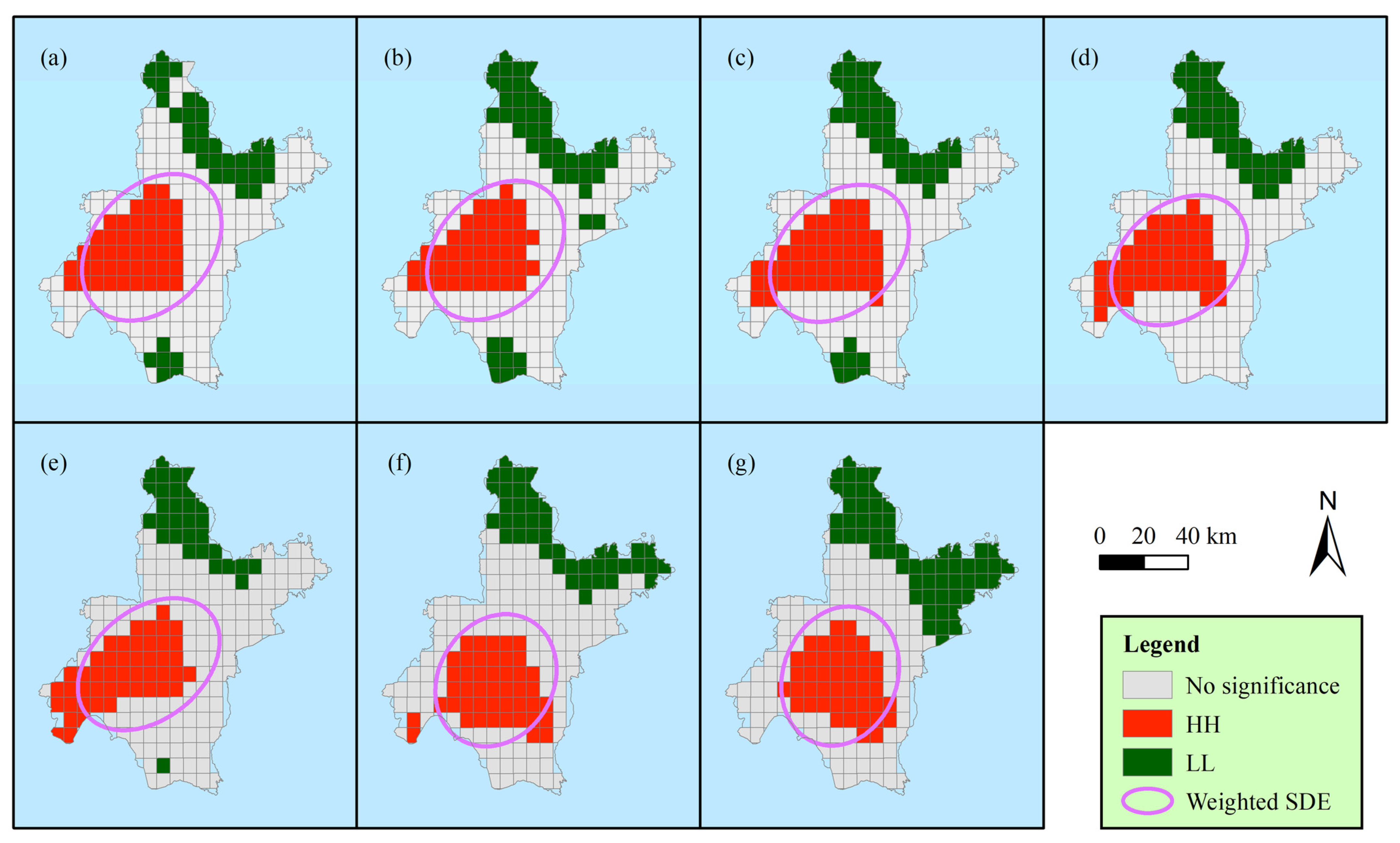
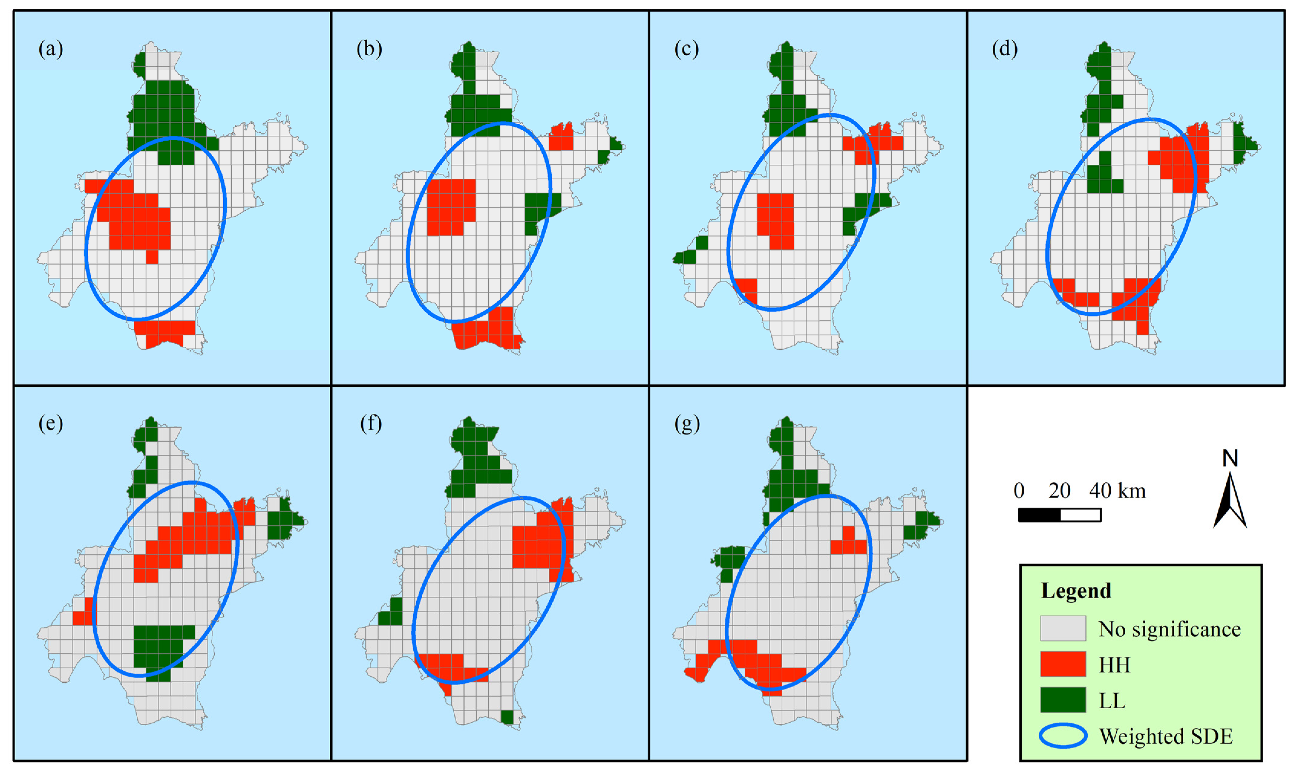
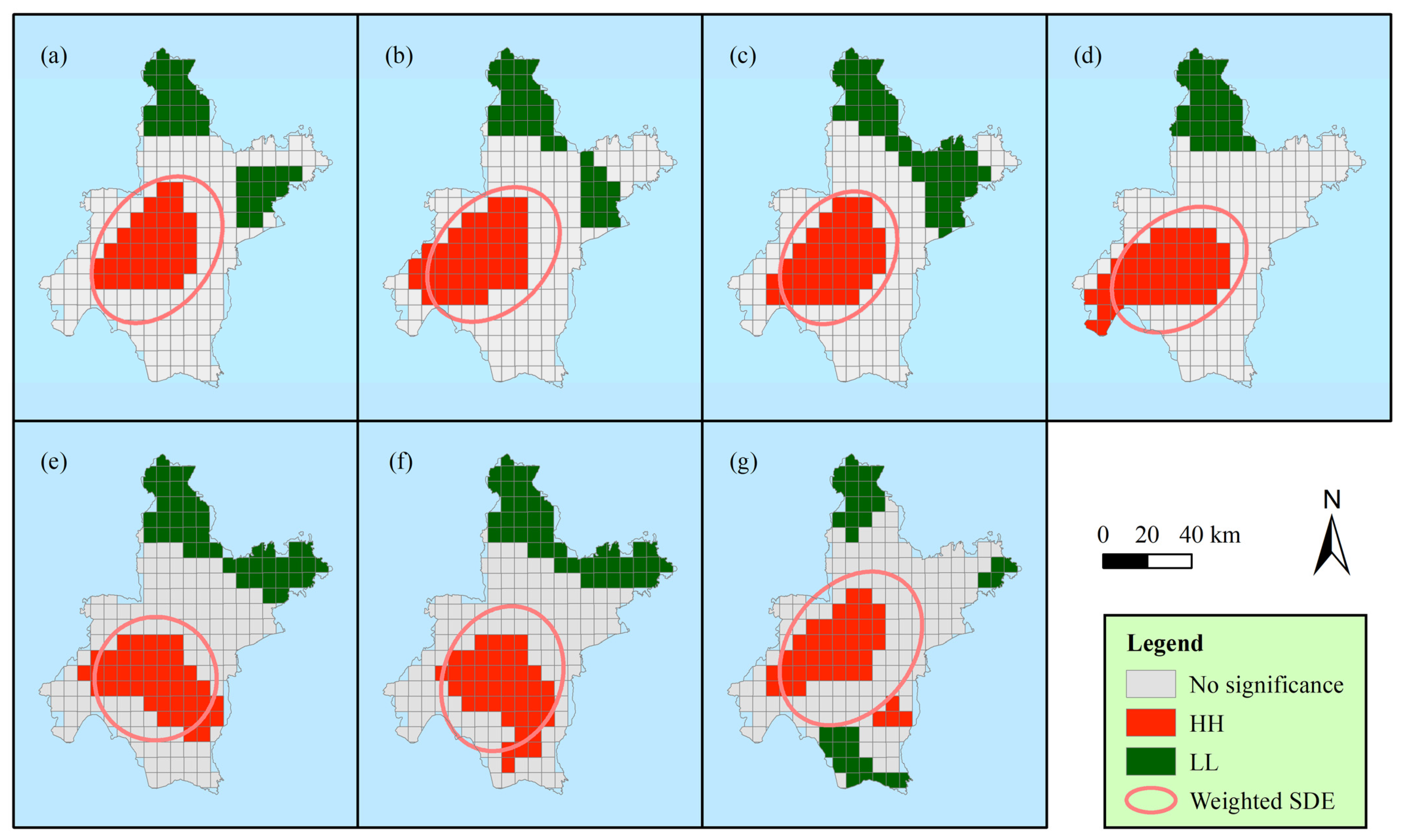
3.2. Local Spatial Pattern of the Thermal Environment

A local spatial analysis of the air temperature distribution is performed at 06:00, 14:00 and 22:00 on the seven days. Identified by calculating local Moran’s I values, the spatial clusters and the outliers of the grid points at the three time points are, respectively, shown in Figure 6, Figure 7 and Figure 8. Only the HH and LL clusters are of statistical significance in the study area at the three time points on all the seven days. The areas, except for the HH and LL clusters, are of no significance. These results indicate that the air temperature distribution has similarly high or low values in neighboring zones; there is no grid point with high air temperature surrounded by grid points with low air temperature nor grid point with low air temperature surrounded by grid points with high air temperature. This also implies that the air temperature of a grid point is affected by the surrounding points.
As seen from Figure 6, the local spatial patterns of the thermal characteristic at 06:00 on seven days mostly overlap, especially on 18 and 19 July. As for 22:00 (Figure 8), the local spatial patterns from 17 July to 19 July mostly overlap and those on 21 and 22 July mostly overlap. Additionally, the overlap proportion of the HH clusters at 06:00 and 22:00 is large in general. However, the HH clusters at 14:00 are substantially different from those at 06:00 and 22:00. Additionally, the corresponding weighted SDEs are displayed in Figure 6, Figure 7 and Figure 8. It can be seen that the results of the SDE analysis are consistent with the local spatial pattern analysis. The shape, position, and size of the weighted SDEs at 06:00 and 22:00 are dominantly determined by the distribution of the HH cluster.
A further analysis regarding the land uses is illustrated in Figure 9, which shows the proportions of the land uses within the HH clusters, LL clusters and no significance clusters. In the HH clusters (Figure 9a), there are four time points at which the proportion of impervious surface is the largest (22:00 on 17 July; 06:00 on 18 July; 06:00 and 22:00 on 19 July), whereas the proportion of the cropland is the largest at the other time points. However, the proportion of cropland is always the largest in the LL clusters (Figure 9b) and no significance clusters (Figure 9c). This probably suggests that cropland is not associated with either high air temperature or low air temperature. The large proportion of cropland in the HH clusters and LL clusters may be due to the fact that the air temperature over cropland is easily affected by neighboring with other land uses. When excluding cropland, as in the HH clusters at 06:00 and 22:00, the proportions of the impervious surface and water bodies are the two largest; additionally, the proportion of impervious surface is generally larger than that of water bodies, except for 22:00 on 20 July and 06:00 on 21 July, which are approximately equal. This may suggest that the HH clusters at 06:00 and 22:00 are associated with the impervious surface and water bodies. Since the proportion of water bodies in the no significance clusters is not very small, this may indicate that the association of the water bodies with the HH clusters at 06:00 and 22:00 is weak. As for the HH clusters at 14:00, the proportion of water bodies is larger than that of impervious surface on five out of seven days; however, these proportions of water bodies is not fairly larger and even sometimes less than those in the no significance clusters. Thus, the water bodies may even be more weakly associated with the HH clusters at 14:00. When considering the land uses in the LL clusters after excluding cropland, the proportion of woodland is always the largest; moreover, the proportion of woodland in the HH clusters and no significance clusters is always very small. This suggests that the LL clusters are strongly associated with woodland (mainly distributed in the northern part of the city).

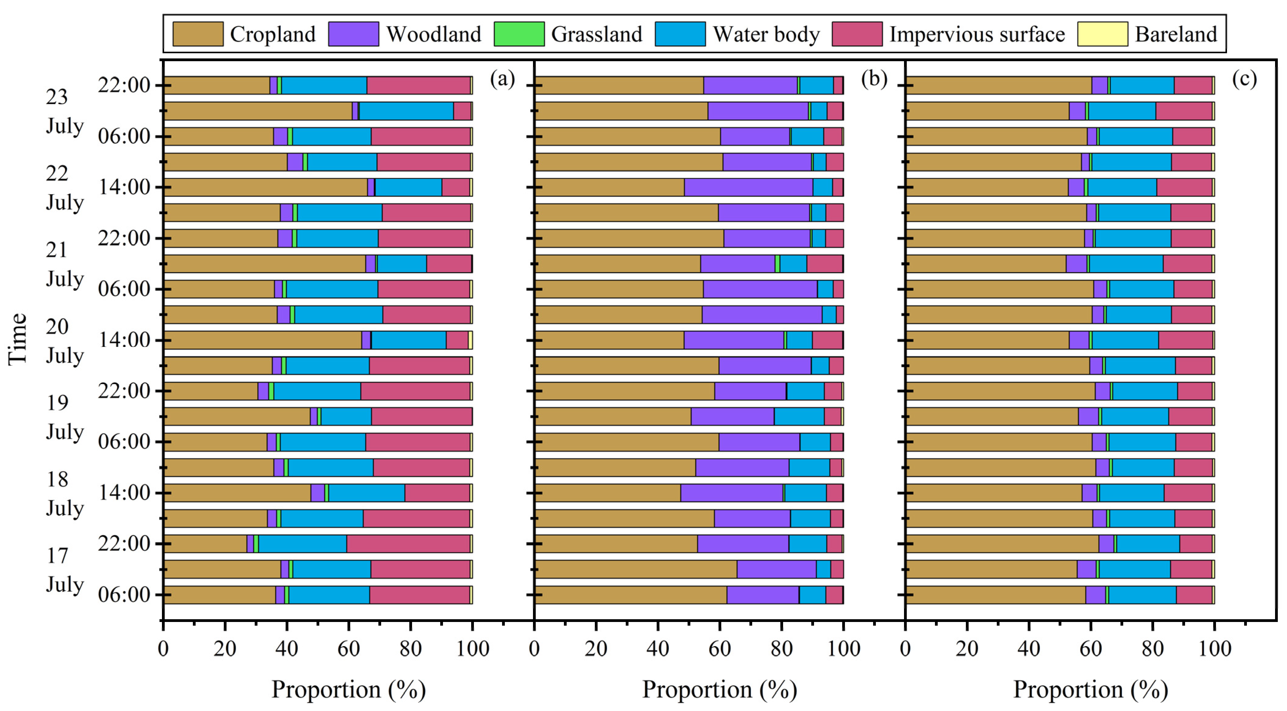
3.3. Land Uses Contributing to Air Temperature Variation

We used a regression analysis to analyze the contribution of land uses to the special distribution of air temperature. We carried out the ordinary least squares (OLS) regression analysis of the air temperature of the grid points with the proportions of land uses with respect to the Thiessen polygons of the grid points. Additionally, stepwise regression technology was used to select the proper variables and eliminate the variables without significance (at the significant level of 0.05).
Among the proportions of the six land use types illustrated in Figure 1b, the main variables contributing to the variation of air temperature are the proportion of woodland area (PWDA), the proportion of water body area (PWBA) and the proportion of impervious surface area (PISA); more details of the OLS regression results are shown in Table 2. The stepwise regression technology can mitigate the collinearity of the predictor variables in the model to some extent. Moreover, the variance inflation factors (VIFs) for the predictors in the final regression model were evaluated and the maximum VIF is presented (Table 2). All the values of the maximum VIF are less than 2, indicating essentially no collinearity. Therefore, the predictor variables could independently predict the value of the dependent variable. The coefficients of PWDA are all significant and all negative at 06:00, 14:00 and 22:00 from 17 July to 23 July, which means that by increasing the proportion of woodland area, the air temperature will decrease. As for PWBA and PISA, both coefficients are significant and positive at 06:00 and 22:00 on the seven days; however, at 14:00, the coefficients of PWBA are only significant on two days and those of PISA are only significant on three days. This means that in the morning and evening, increasing the proportions of water body area and impervious surface area will increase the air temperature. However, at noon, the effects of the water body and the impervious surface may require further consideration, for the coefficients of PWBA and PISA are not always significant.
When considering the fitness of the OLS model varying in time (R2 in Table 2), it can be seen that the R2 value at 22:00 is larger than that at 06:00 each day, and that the R2 value at 06:00 is larger than that at 14:00. With the exception of 22 July, the OLS model can explain more than 50% of the variation in the spatial distribution of air temperature at 22:00; at 06:00, there are three days on which more than 50% of the variation can be explained by the model. However, at 14:00, the model can explain not more than 40% of the variation, with the exception of 17 and 22 July, and even less than 20% on 21 July. This suggests that there are some other factors affecting the spatial distribution of air temperature. Moreover, we used the spatial lag model (SLM) with the same independent variables than for the regression analysis. The results are shown in Table 3. The R2 of the model is very high at all the time points, much larger than that of the OLS model. None of the R2 values at 06:00 and 22:00 are lesser than 0.97; only the R2 values at 14:00 on 19 and 23 July are slightly lesser than 0.90, but also greater than 0.89. This means that the explanation of the SLM is improved. However, the absolute values of the coefficients of the explanatory variables become smaller. This is because some variation of the dependent variable explained by the independent variable is substituted by the spatially lagged term (WTa in Equation (14)). When the absolute value becomes very small and close to zero, it may not even be statistically significantly different from the zero value. As seen from Table 3, all the coefficients with absolute values of less than 0.1 are not significant. Two of the coefficients of PISA that are significant in the OLS model become not significant. Even the coefficients of PWBA all become not significant. Conversely, the Lag coefficients of the SLM are very high (higher than 0.95) and extremely significant at all the time points, which indicates that the contribution of spatial autocorrelation to the spatial variation of air temperature is very high and that the air temperature of one grid point is greatly affected by its neighboring points. This implies that the effect of spatial diffusion is significant in the spatial distribution of air temperature.

4. Discussion

4.1. Advantage of the UHI Index

Figure 10 displays the standard deviation of air temperature (Ta-SD) of the grid points, its trend generally corresponding to that of the UHI index (Figure 4). It may be supposed that the UHI index is simply determined by the variation of air temperature with respect to the grid points. However, this is not exactly true. In order to illustrate this issue, we first calculated the difference in the UHI index and the difference in the Ta-SD in 2 h steps. We then calculated the quotient of the differences, which is shown in Figure 10. As it can be seen, the difference quotient is positive most of the time, but there are still some times when the difference quotient is negative. This means that at some time points, not very few, the change trend of the UHI index is opposite to that of the Ta-SD. As the UHI index is derived from an SDE analysis, it considers not only the value distribution of air temperature, but also the spatial distribution. With the same Ta-SD, the spatial distribution could be different, so the values of the UHI index may be distinct. In specific situations, with the same Ta-SD, an area may present the state of heat island or the state of cool island. However, these situations can be distinguished by the UHI index, for its value of the former is greater than 1 and that of the latter less than 1. Thus, the UHI index has an advantage in characterizing the spatial distribution of the thermal environment and the UHI effect.

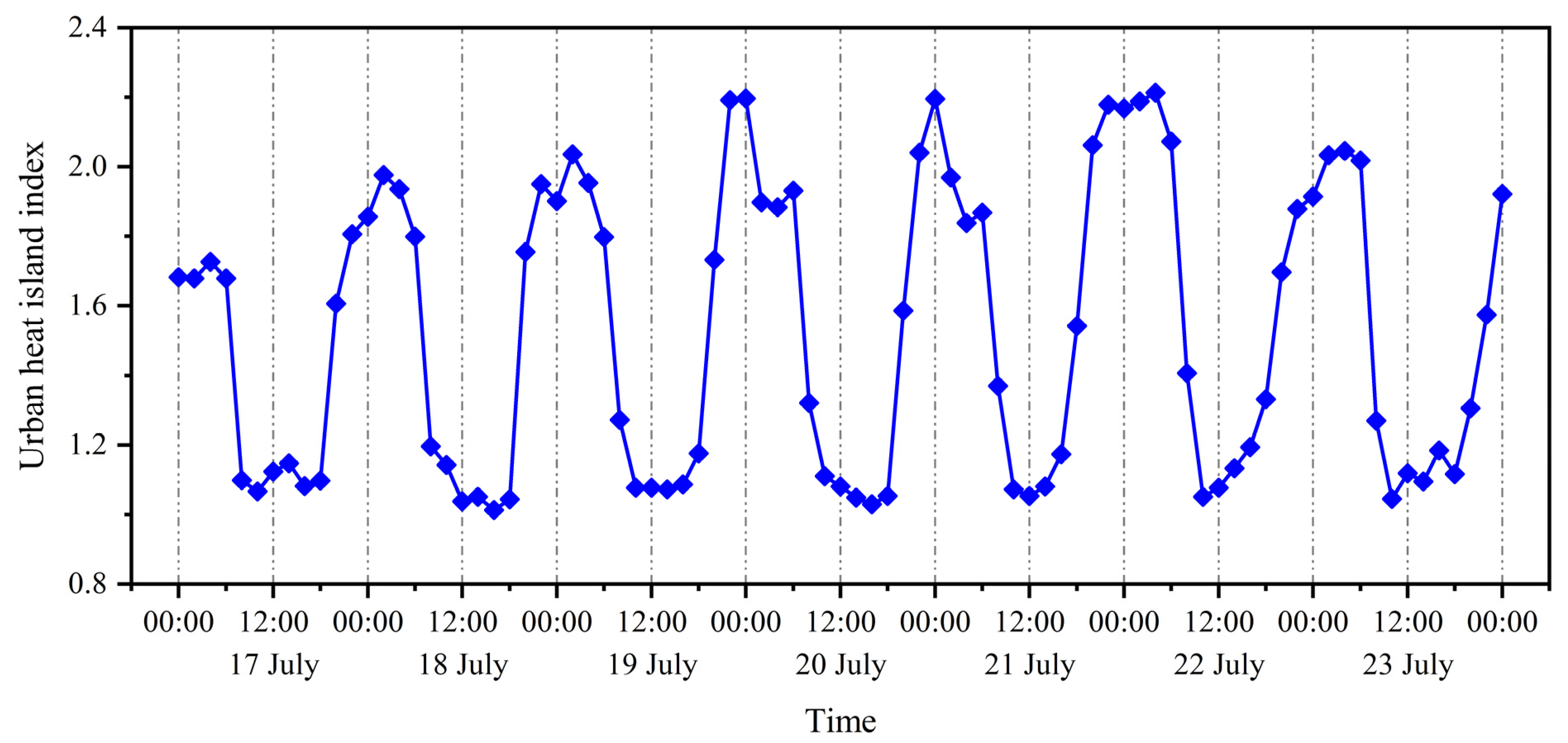
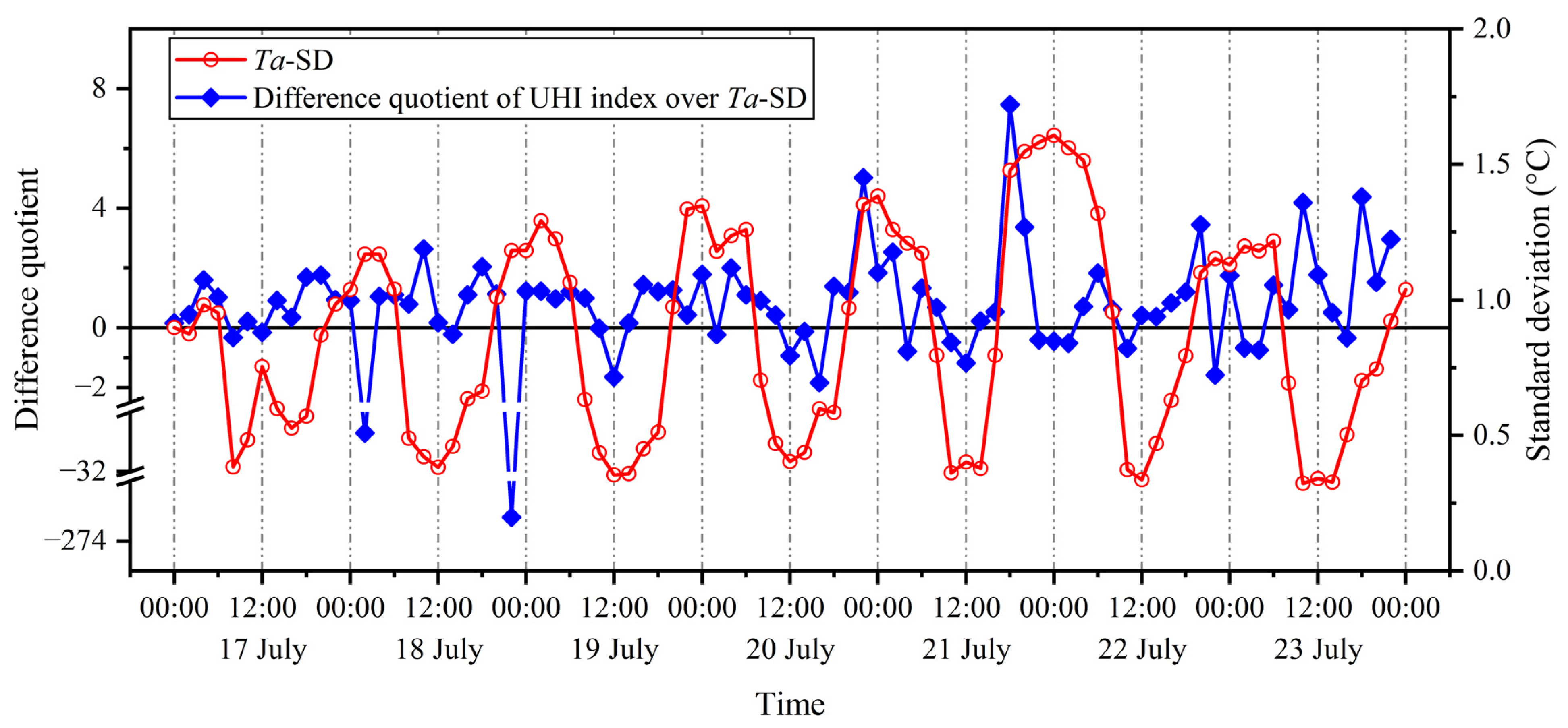
4.2. Thermal Environment in Relation to Weather Condition

The weather conditions of the seven days on which we analyzed the thermal environmental characteristics are cloudy and sunny. As it can be seen, the UHI index from 10:00 to 16:00 does not vary much on these seven days. However, the values of the UHI index at 22:00 and at 24:00 on the three sunny days are all greater than those on the four cloudy days. These results are in accordance with the other literature. There is wide consensus that the UHI effect is strong during the nighttime but weak or even disappears during the daytime [45,46,47,48]. Thus, the influence of weather conditions on the UHI effect is slight during the daytime. However, during the nighttime, previous studies have demonstrated that that the UHI intensity in clear conditions is evidently greater than in overcast conditions during the nighttime [47,49,50].
Conventionally, UHI intensity is usually the difference between urban peak air temperatures and rural air temperatures. In this study, the curve of the UHI index reflects that the air temperature difference between urban center and the outskirts of the city during the nighttime on sunny days is generally greater than that on cloudy days, implying that the spatial heterogeneity of thermal environmental characteristics increases in sunny days.

4.3. Limitations of the Regression Models

In this study, we attribute the spatial variation of the air temperature to local land uses by using a regression analysis. In fact, wind is also an important factor affecting air temperature, which is not considered in the regression model. This may be a reason why the coefficients of the determination with respect to the OLS model are not very satisfactory. Yet, the magnitude of the variation in air temperature explained by the land use regression model is also not very satisfactory in previous studies [51,52,53,54]. However, it is difficult to consider the contribution of wind in a global regression model, for the effect of wind on local air temperature is complex. Even if the wind remains in a constant direction, it may decrease the air temperature in one local area but may increase the air temperature in another local area, not to mention that the wind’s direction frequently changes. Thus, it may not be suitable to consider the contribution of wind to local air temperature in space when using the OLS model. When the SLM is adopted, the coefficients of the determination greatly improve. Since the SLM can reflect the effect of spatial diffusion, it can be supposed that the model takes into account the effect of the wind to some extent. However, this comes at the cost of losing the explanation of the local independent variables, namely the proportion of land uses, for the absolute values of the regression coefficients become smaller and some of them are even without significance.

5. Conclusions

In the light of the ambiguous measurements in UHI intensity and the scarce studies on the spatial characteristics’ evolution of the urban thermal environment with the high temporal resolution during a day, this study introduces the SDE method to depict the general spatial character of the urban thermal environment and constructs an UHI index to evaluate the UHI intensity based on the SDE. Taking the city of Wuhan as a study area, the results illustrate that the UHI index can effectively represent the general characteristics of the thermal environment in the study area. The trends of the UHI intensity generally decrease from midnight to midday, and generally increase from midday to evening. The local spatial pattern analysis through local Moran’s I shows that there are only high–high clusters and low–low clusters of air temperature with statistical significance in the study area. The former clusters are mainly associated with the imperious surface, and are also associated with water bodies in the morning and the evening. The latter clusters are mainly associated with woodland. This can be further demonstrated by a regression analysis. The regression analysis of the SLM also indicates that the effect of spatial diffusion has a significant influence on the distribution of air temperature in space.
Furthermore, the regression analysis indicates that the effects of water body on air temperature are mostly not statistically significant at noon according to the OLS model and are even all insignificant in the morning, noon and evening according to the SLM model. Nevertheless, woodland always has a cooling effect in the morning, at noon and in the evening, implying that increasing the vegetation may be the most effective strategy to mitigate the urban thermal environment. The regression results also show that the OLS model could not fit the spatial distribution of air temperature well enough, while the fitness of the SLM is greatly improved. However, the explanation of the proportion of the local land uses accounting for the spatial variation of air temperature becomes lower. An improved model is still required to explain the spatial distribution of the urban air temperature.

Author Contributions

Design of the research, W.S. and R.X.; methodology and data processing, W.S.; writing of the article, W.S. and J.H.; verification of the results, X.S. All authors have read and agreed to the published version of the manuscript.

Funding

This research was funded by National Natural Science Foundation of China (NSFC), grant number 41701179.

Data Availability Statement

Data is contained within the article.

Conflicts of Interest

The authors declare no conflict of interest.

References

  1. Jedlovec, G.; Crane, D.; Quattrochi, D. Urban heat wave hazard and risk assessment. Results Phys. 2017, 7, 4294–4295. [Google Scholar] [CrossRef]
  2. He, B.J.; Wang, J.S.; Liu, H.M.; Ulpiani, G. Localized synergies between heat waves and urban heat islands: Implications on human thermal comfort and urban heat management. Environ. Res. 2021, 193, 18. [Google Scholar] [CrossRef]
  3. Li, D.; Bou-Zeid, E. Synergistic Interactions between Urban Heat Islands and Heat Waves: The Impact in Cities Is Larger than the Sum of Its Parts. J. Appl. Meteorol. Climatol. 2013, 52, 2051–2064. [Google Scholar] [CrossRef] [Green Version]
  4. Tan, J.G.; Zheng, Y.F.; Tang, X.; Guo, C.Y.; Li, L.P.; Song, G.X.; Zhen, X.R.; Yuan, D.; Kalkstein, A.J.; Li, F.R.; et al. The urban heat island and its impact on heat waves and human health in Shanghai. Int. J. Biometeorol. 2010, 54, 75–84. [Google Scholar] [CrossRef] [PubMed]
  5. Grimm, N.B.; Faeth, S.H.; Golubiewski, N.E.; Redman, C.L.; Wu, J.G.; Bai, X.M.; Briggs, J.M. Global change and the ecology of cities. Science 2008, 319, 756–760. [Google Scholar] [CrossRef] [Green Version]
  6. Chen, X.L.; Zhao, H.M.; Li, P.X.; Yin, Z.Y. Remote sensing image-based analysis of the relationship between urban heat island and land use/cover changes. Remote Sens. Environ. 2006, 104, 133–146. [Google Scholar] [CrossRef]
  7. Xian, G.; Shi, H.; Auch, R.; Gallo, K.; Zhou, Q.; Wu, Z.T.; Kolian, M. The effects of urban land cover dynamics on urban heat Island intensity and temporal trends. GISci. Remote Sens. 2021, 58, 501–515. [Google Scholar] [CrossRef]
  8. Radhi, H.; Fikry, F.; Sharples, S. Impacts of urbanisation on the thermal behaviour of new built up environments: A scoping study of the urban heat island in Bahrain. Landsc. Urban Plan. 2013, 113, 47–61. [Google Scholar] [CrossRef]
  9. Connors, J.P.; Galletti, C.S.; Chow, W.T.L. Landscape configuration and urban heat island effects: Assessing the relationship between landscape characteristics and land surface temperature in Phoenix, Arizona. Landscape Ecol. 2013, 28, 271–283. [Google Scholar] [CrossRef]
  10. Hart, M.; Sailor, D. Quantifying the influence of land-use and surface characteristics on spatial variability in the urban heat island. Theor. Appl. Climatol. 2009, 95, 397–406. [Google Scholar] [CrossRef]
  11. Morini, E.; Touchaei, A.G.; Castellani, B.; Rossi, F.; Cotana, F. The Impact of Albedo Increase to Mitigate the Urban Heat Island in Terni (Italy) Using the WRF Model. Sustainability 2016, 8, 999. [Google Scholar] [CrossRef] [Green Version]
  12. Zhang, Y.S.; Wang, X.Q.; Balzter, H.; Qiu, B.W.; Cheng, J.Y. Directional and Zonal Analysis of Urban Thermal Environmental Change in Fuzhou as an Indicator of Urban Landscape Transformation. Remote Sens. 2019, 11, 2810. [Google Scholar] [CrossRef] [Green Version]
  13. Maimaitiyiming, M.; Ghulam, A.; Tiyip, T.; Pla, F.; Latorre-Carmona, P.; Halik, U.; Sawut, M.; Caetano, M. Effects of green space spatial pattern on land surface temperature: Implications for sustainable urban planning and climate change adaptation. ISPRS-J. Photogramm. Remote Sens. 2014, 89, 59–66. [Google Scholar] [CrossRef] [Green Version]
  14. Kong, F.H.; Yin, H.W.; James, P.; Hutyra, L.R.; He, H.S. Effects of spatial pattern of greenspace on urban cooling in a large metropolitan area of eastern China. Landsc. Urban Plan. 2014, 128, 35–47. [Google Scholar] [CrossRef]
  15. Masoudi, M.; Tan, P.Y. Multi-year comparison of the effects of spatial pattern of urban green spaces on urban land surface temperature. Landsc. Urban Plan. 2019, 184, 44–58. [Google Scholar] [CrossRef]
  16. Nakayama, T.; Hashimoto, S. Analysis of the ability of water resources to reduce the urban heat island in the Tokyo megalopolis. Environ. Pollut. 2011, 159, 2164–2173. [Google Scholar] [CrossRef]
  17. Lin, Y.; Wang, Z.F.; Jim, C.Y.; Li, J.B.; Deng, J.S.; Liu, J.G. Water as an urban heat sink: Blue infrastructure alleviates urban heat island effect in mega-city agglomeration. J. Clean. Prod. 2020, 262, 8. [Google Scholar] [CrossRef]
  18. Steeneveld, G.J.; Koopmans, S.; Heusinkveld, B.G.; Theeuwes, N.E. Refreshing the role of open water surfaces on mitigating the maximum urban heat island effect. Landsc. Urban Plan. 2014, 121, 92–96. [Google Scholar] [CrossRef]
  19. Oke, T.R.; Mills, G.; Christen, A.; Voogt, J.A. Urban Climates, 1st ed.; Cambridge University Press: Cambridge, UK, 2017; pp. 197–200. [Google Scholar]
  20. Schwarz, N.; Schlink, U.; Franck, U.; Grossmann, K. Relationship of land surface and air temperatures and its implications for quantifying urban heat island indicators-An application for the city of Leipzig (Germany). Ecol. Indic. 2012, 18, 693–704. [Google Scholar] [CrossRef]
  21. Sun, T.; Sun, R.H.; Chen, L.D. The Trend Inconsistency between Land Surface Temperature and Near Surface Air Temperature in Assessing Urban Heat Island Effects. Remote Sens. 2020, 12, 1271. [Google Scholar] [CrossRef]
  22. Venter, Z.S.; Chakraborty, T.; Lee, X.H. Crowdsourced air temperatures contrast satellite measures of the urban heat island and its mechanisms. Sci. Adv. 2021, 7, 9. [Google Scholar] [CrossRef] [PubMed]
  23. Azevedo, J.A.; Chapman, L.; Muller, C.L. Quantifying the Daytime and Night-Time Urban Heat Island in Birmingham, UK: A Comparison of Satellite Derived Land Surface Temperature and High Resolution Air Temperature Observations. Remote Sens. 2016, 8, 153. [Google Scholar] [CrossRef] [Green Version]
  24. Oke, T.R. City size and urban heat island. Atmos. Environ. 1973, 7, 769–779. [Google Scholar] [CrossRef]
  25. Earl, N.; Simmonds, I.; Tapper, N. Weekly cycles in peak time temperatures and urban heat island intensity. Environ. Res. Lett. 2016, 11, 10. [Google Scholar] [CrossRef]
  26. Stewart, I.D. A systematic review and scientific critique of methodology in modern urban heat island literature. Int. J. Climatol. 2011, 31, 200–217. [Google Scholar] [CrossRef]
  27. Du, H.Y.; Wang, D.D.; Wang, Y.Y.; Zhao, X.L.; Qin, F.; Jiang, H.; Cai, Y.L. Influences of land cover types, meteorological conditions, anthropogenic heat and urban area on surface urban heat island in the Yangtze River Delta Urban Agglomeration. Sci. Total Environ. 2016, 571, 461–470. [Google Scholar] [CrossRef]
  28. Cui, Y.P.; Xu, X.L.; Dong, J.W.; Qin, Y.C. Influence of Urbanization Factors on Surface Urban Heat Island Intensity: A Comparison of Countries at Different Developmental Phases. Sustainability 2016, 8, 706. [Google Scholar] [CrossRef] [Green Version]
  29. Deilami, K.; Kamruzzaman, M.; Hayes, J.F. Correlation or Causality between Land Cover Patterns and the Urban Heat Island Effect? Evidence from Brisbane, Australia. Remote Sens. 2016, 8, 716. [Google Scholar] [CrossRef] [Green Version]
  30. Estoque, R.C.; Murayama, Y.; Myint, S.W. Effects of landscape composition and pattern on land surface temperature: An urban heat island study in the megacities of Southeast Asia. Sci. Total Environ. 2017, 577, 349–359. [Google Scholar] [CrossRef]
  31. Yao, R.; Wang, L.C.; Huang, X.; Zhang, W.W.; Li, J.L.; Niu, Z.G. Interannual variations in surface urban heat island intensity and associated drivers in China. J. Environ. Manag. 2018, 222, 86–94. [Google Scholar] [CrossRef]
  32. Yao, R.; Wang, L.C.; Huang, X.; Gong, W.; Xia, X.G. Greening in Rural Areas Increases the Surface Urban Heat Island Intensity. Geophys. Res. Lett. 2019, 46, 2204–2212. [Google Scholar] [CrossRef]
  33. Han, S.; Liu, B.C.; Shi, C.X.; Liu, Y.; Qiu, M.J.; Sun, S. Evaluation of CLDAS and GLDAS Datasets for Near-Surface Air Temperature over Major Land Areas of China. Sustainability 2020, 12, 4311. [Google Scholar] [CrossRef]
  34. Huang, X.L.; Han, S.; Shi, C.X. Evaluation of Three Air Temperature Reanalysis Datasets in the Alpine Region of the Qinghai-Tibet Plateau. Remote Sens. 2022, 14, 4447. [Google Scholar] [CrossRef]
  35. Leng, P.; Li, Z.L.; Duan, S.B.; Gao, M.F.; Huo, H.Y. A practical approach for deriving all-weather soil moisture content using combined satellite and meteorological data. ISPRS-J. Photogramm. Remote Sens. 2017, 131, 40–51. [Google Scholar] [CrossRef]
  36. Zhou, W.; Peng, B.; Shi, J.C.; Wang, T.X.; Dhital, Y.P.; Yao, R.Z.; Yu, Y.C.; Lei, Z.T.; Zhao, R. Estimating High Resolution Daily Air Temperature Based on Remote Sensing Products and Climate Reanalysis Datasets over Glacierized Basins: A Case Study in the Langtang Valley, Nepal. Remote Sens. 2017, 9, 959. [Google Scholar] [CrossRef] [Green Version]
  37. Rao, Y.H.; Liang, S.L.; Wang, D.D.; Yu, Y.Y.; Song, Z.; Zhou, Y.; Shen, M.G.; Xu, B.Q. Estimating daily average surface air temperature using satellite land surface temperature and top-of-atmosphere radiation products over the Tibetan Plateau. Remote Sens. Environ. 2019, 234, 14. [Google Scholar] [CrossRef]
  38. Chen, Y.; Liang, S.L.; Ma, H.; Li, B.; He, T.; Wang, Q. An all-sky 1 km daily land surface air temperature product over mainland China for 2003–2019 from MODIS and ancillary data. Earth Syst. Sci. Data 2021, 13, 4241–4261. [Google Scholar] [CrossRef]
  39. Ran, Y.H.; Li, X.; Lu, L. Evaluation of four remote sensing based land cover products over China. Int. J. Remote Sens. 2010, 31, 391–401. [Google Scholar] [CrossRef]
  40. Lefever, D.W. Measuring geographic concentration by means of the standard deviational ellipse. Am. J. Sociol. 1926, 32, 88–94. [Google Scholar] [CrossRef]
  41. Johnson, D.P.; Wilson, J.S. The socio-spatial dynamics of extreme urban heat events: The case of heat-related deaths in Philadelphia. Appl. Geogr. 2009, 29, 419–434. [Google Scholar] [CrossRef]
  42. Xu, J.H.; Zhao, Y.; Zhong, K.W.; Zhang, F.F.; Liu, X.L.; Sun, C.G. Measuring spatio-temporal dynamics of impervious surface in Guangzhou, China, from 1988 to 2015, using time-series Landsat imagery. Sci. Total Environ. 2018, 627, 264–281. [Google Scholar] [CrossRef] [PubMed]
  43. Anselin, L. Local indicators of spatial association—LISA. Geogr. Anal. 1995, 27, 93–115. [Google Scholar] [CrossRef]
  44. Anselin, L.; Rey, S. Properties of tests for spatial dependence in linear-regression models. Geogr. Anal. 1991, 23, 112–131. [Google Scholar] [CrossRef]
  45. Oke, T.R. The energetic basis of the urban heat-island. Q. J. R. Meteorol. Soc. 1982, 108, 1–24. [Google Scholar] [CrossRef]
  46. Basara, J.B.; Hall, P.K.; Schroeder, A.J.; Illston, B.G.; Nemunaitis, K.L. Diurnal cycle of the Oklahoma City urban heat island. J. Geophys. Res.-Atmos. 2008, 113, 16. [Google Scholar] [CrossRef]
  47. Wolters, D.; Brandsma, T. Estimating the Urban Heat Island in Residential Areas in the Netherlands Using Observations by Weather Amateurs. J. Appl. Meteorol. Climatol. 2012, 51, 711–721. [Google Scholar] [CrossRef]
  48. Hardin, A.W.; Liu, Y.; Cao, G.; Vanos, J.K. Urban heat island intensity and spatial variability by synoptic weather type in the northeast U.S. Urban Clim. 2018, 24, 747–762. [Google Scholar] [CrossRef]
  49. Morris, C.J.G.; Simmonds, I.; Plummer, N. Quantification of the influences of wind and cloud on the nocturnal urban heat island of a large city. J. Appl. Meteorol. 2001, 40, 169–182. [Google Scholar] [CrossRef]
  50. Ngarambe, J.; Oh, J.W.; Su, M.A.; Santamouris, M.; Yun, G.Y. Influences of wind speed, sky conditions, land use and land cover characteristics on the magnitude of the urban heat island in Seoul: An exploratory analysis. Sust. Cities Soc. 2021, 71, 22. [Google Scholar] [CrossRef]
  51. Myint, S.W.; Brazel, A.; Okin, G.; Buyantuyev, A. Combined Effects of Impervious Surface and Vegetation Cover on Air Temperature Variations in a Rapidly Expanding Desert City. GISci. Remote Sens. 2010, 47, 301–320. [Google Scholar] [CrossRef]
  52. Schatz, J.; Kucharik, C.J. Urban climate effects on extreme temperatures in Madison, Wisconsin, USA. Environ. Res. Lett. 2015, 10, 13. [Google Scholar] [CrossRef] [Green Version]
  53. Coseo, P.; Larsen, L. Accurate Characterization of Land Cover in Urban Environments: Determining the Importance of Including Obscured Impervious Surfaces in Urban Heat Island Models. Atmosphere 2019, 10, 347. [Google Scholar] [CrossRef] [Green Version]
  54. Tsin, P.K.; Knudby, A.; Krayenhoff, E.S.; Brauer, M.; Henderson, S.B. Land use regression modeling of microscale urban air temperatures in greater Vancouver, Canada. Urban Clim. 2020, 32, 12. [Google Scholar] [CrossRef]
Figure 1. Study area. (a) Grid points of the air temperature; (b) Land uses.
Remotesensing 14 06084 g001
Figure 2. The mean air temperature isotherm of an extended area including the city of Wuhan from 17 July to 23 July. (a) Nighttime; (b) daytime.
Remotesensing 14 06084 g002
Figure 3. The mean air temperature profiles along line AB.
Remotesensing 14 06084 g003
Figure 4. UHI index of the city of Wuhan in the summer of 2018.
Remotesensing 14 06084 g004
Figure 5. The SDEs of the city of Wuhan. (a) 17 July; (b) 18 July; (c) 19 July; (d) 20 July; (e) 21 July; (f) 22 July; (g) 23 July.
Remotesensing 14 06084 g005
Figure 6. Local spatial pattern of the air temperature at 06:00 (significant level at 0.05). (a) 17 July; (b) 18 July; (c) 19 July; (d) 20 July; (e) 21 July; (f) 22 July; (g) 23 July.
Remotesensing 14 06084 g006
Figure 7. Local spatial pattern of the air temperature at 14:00 (significant level at 0.05). (a) 17 July; (b) 18 July; (c) 19 July; (d) 20 July; (e) 21 July; (f) 22 July; (g) 23 July.
Remotesensing 14 06084 g007
Figure 8. Local spatial pattern of the air temperature at 22:00 (significant level at 0.05). (a) 17 July; (b) 18 July; (c) 19 July; (d) 20 July; (e) 21 July; (f) 22 July; (g) 23 July.
Remotesensing 14 06084 g008
Figure 9. Proportions of land uses in the local spatial patterns. (a) HH cluster; (b) LL cluster; (c) no significance cluster.
Remotesensing 14 06084 g009
Figure 10. Comparison of UHI index and the standard deviation of the air temperature (Ta-SD) in the study area.
Remotesensing 14 06084 g010
Table 1. Weather conditions of the study area in the study period.
DateWeather Condition
17 JulyCloudy
18 JulyCloudy
19 JulySunny
20 JulySunny
21 JulySunny
22 JulyCloudy
23 JulyCloudy
Table 2. Coefficients of the OLS regression with respect to air temperature.
DateTimeConstantPWDAPWBAPISAMax VIFR2Adjusted R2
17 July06:0026.77 ***−1.202 ***1.223 ***2.594 ***1.2070.4300.422
14:0035.67 ***−0.963 ***1.026 ***1.145 ***1.2070.4080.399
22:0030.33 ***−2.247 ***1.175 ***2.756 ***1.2070.6140.608
18 July06:0027.12 ***−1.590 ***1.279 ***3.009 ***1.2070.4990.492
14:0037.02 ***−1.517 ***---0.3290.326
22:0030.82 ***−2.860 ***1.287 ***2.877 ***1.2070.5550.548
19 July06:0027.19 ***−1.749 ***1.488 ***2.995 ***1.2070.5220.515
14:0037.45 ***−1.061 ***-0.327 **1.0680.3350.328
22:0030.75 ***−2.710 ***1.749 ***3.367 ***1.2070.5230.516
20 July06:0027.10 ***−2.375 ***1.742 ***3.160 ***1.2070.5040.497
14:0037.68 ***−1.568 ***-−0.634 ***1.0680.3730.367
22:0030.47 ***−3.102 ***2.048 ***2.960 ***1.2070.5460.539
21 July06:0027.34 ***−2.751 ***1.630 ***2.902 ***1.2070.5910.585
14:0038.34 ***−0.895 ***---0.1690.165
22:0030.99 ***−3.622 ***2.528 ***3.152 ***1.2070.5260.519
22 July06:0026.84 ***−2.669 ***2.176 ***2.658 ***1.2070.4870.479
14:0036.63 ***−1.862 ***---0.4730.471
22:0030.44 ***−2.325 ***1.862 ***2.431 ***1.2070.4950.487
23 July06:0026.97 ***−2.218 ***1.847 ***2.715 ***1.2070.4630.455
14:0036.72 ***−0.923 ***0.362 ***-1.1130.3550.349
22:0030.15 ***−2.300 ***0.882 ***2.147 ***1.2070.5350.528
*** Significant at p < 0.001, ** significant at p < 0.01.
Table 3. Coefficients of the SLM regression with respect to the air temperature.
DateTimeLag
Coefficient
ConstantPWDAPWBAPISAR2
17 July06:000.986 ***0.358 *−0.264 ***0.0680.154 *0.977
14:000.962 ***1.368 ***−0.289 ***0.0710.0680.962
22:000.965 ***1.057 ***−0.373 ***0.0400.221 ***0.986
18 July06:000.984 ***0.429 *−0.299 ***0.0510.199 **0.981
14:000.964 ***1.356 ***−0.395 ***--0.934
22:000.972 ***0.862 ***−0.388 ***0.0160.202 ***0.990
19 July06:000.982 ***0.476 **−0.329 ***0.0490.184 **0.982
14:000.956 ***1.682 ***−0.388 ***-−0.0090.892
22:000.980 ***0.611 **−0.348 ***0.0290.235 ***0.990
20 July06:000.981 ***0.497 **−0.341 ***0.0410.214 **0.985
14:000.962 ***1.456 ***−0.420 ***-−0.119 **0.934
22:000.970 ***0.894 **−0.301 ***0.0990.254 ***0.989
21 July06:000.963 ***1.005 ***−0.404 ***0.0770.215 ***0.987
14:000.973 ***1.074 **−0.331 ***--0.900
22:000.979 ***0.643 **−0.329 ***0.0410.207 ***0.993
22 July06:000.980 ***0.514 **−0.322 ***0.0990.188 **0.989
14:000.941 ***2.167 ***−0.457 ***--0.941
22:000.974 ***0.793 **−0.340 ***−0.0030.213 ***0.984
23 July06:000.980 ***0.531**−0.320 ***−0.0040.191 ***0.990
14:000.947 ***1.952 ***−0.334 ***0.011-0.891
22:000.969 ***0.927 **−0.353 ***0.0350.134 *0.970
*** Significant at p < 0.001, ** significant at p < 0.01, * significant at p < 0.05.
Publisher’s Note: MDPI stays neutral with regard to jurisdictional claims in published maps and institutional affiliations.

