Monitoring Short-Term Morphobathymetric Change of Nearshore Seafloor Using Drone-Based Multispectral Imagery

Abstract

Short-term changes in shallow bathymetry affect the coastal zone, and therefore their monitoring is an essential task in coastal planning projects. This study provides a novel approach for monitoring shallow bathymetry changes based on drone multispectral imagery. Particularly, we apply a shallow water inversion algorithm on two composite multispectral datasets, being acquired five months apart in a small Mediterranean sandy embayment (Chania, Greece). Initially, we perform radiometric corrections using proprietary software, and following that we combine the bands from standard and multispectral cameras, resulting in a six-band composite image suitable for applying the shallow water inversion algorithm. Bathymetry inversion results showed good correlation and low errors (<0.3 m) with sonar measurements collected with an uncrewed surface vehicle (USV). Bathymetry maps and true-color orthomosaics assist in identifying morphobathymetric features representing crescentic bars with rip channel systems. The temporal bathymetry and true-color data reveal important erosional and depositional patterns, which were developed under the impact of winter storms. Furthermore, bathymetric profiles show that the crescentic bar appears to migrate across and along-shore over the 5-months period. Drone-based multispectral imagery proves to be an important and cost-effective tool for shallow seafloor mapping and monitoring when it is combined with shallow water analytical models.

1. Introduction

The shallow coastal seafloor is constantly under the influence of waves and currents, thus its surface changes rapidly over different spatio-/temporal scales. At the same time, shallow seafloor covers a wide area globally where major economic and other activities take place. Consequently, mapping and monitoring of shallow seafloor bathymetry is a fundamental strategy for several projects including, but not limited to, maritime safety, coastal vulnerability [1,2,3] and coastal planning [4,5,6]. However, obtaining bathymetry data at the coastal zone is not as straightforward as it is in continental shelf mapping, and it depends on many environmental factors. This is thought to be due to the fact that: (a) shallow seafloor changes quickly, and thus bathymetry collected today is often no longer valid even after a short period of time; and (b) traditional sonar surveying is unable to provide full coverage at high spatial resolution (<1 m) in a time- and cost-effective way. Therefore, new techniques were introduced for efficient shallow bathymetry mapping, covering broad shallow areas at frequent (i.e., daily, weekly) time intervals [7,8,9]. These techniques include active or passive optical sensors deployed on airborne or satellite platforms. Such data are suitable for mapping areas with increased water transparency where seafloor is visible [8,10]. In the case of turbid waters, bathymetry inversion based on wave geometry and celerity has also been applied as an alternative technique to sonar mapping [11,12]. The most recognized optical technique for shallow seafloor mapping is light detection and ranging (LIDAR). LIDAR sensors have been widely applied in shallow seafloor mapping studies due to their increased spatial resolution and data density, along with their extensive coverage [13,14,15,16]. Particularly, airborne bathymetric LIDAR is the leading technology for studying nearshore bathymetry, providing meter-scale horizontal accuracy and centimeter-scale vertical accuracy over large areas of coastal seafloor [15,17]. However, the cost of LIDAR sensors and the costs and logistic effort for acquiring bathymetric LIDAR data are often limiting factors [18] that hinder the accessibility of this kind of technology to low-budget projects. Applications based on multi- or hyperspectral imagery are considered as an alternative to LIDAR for shallow bathymetry retrieval. Deriving shallow bathymetry using passive optical imagery is a field of ongoing research, which has been greatly expanded in recent years as it provides extended scale coverage and at relatively low-cost compared to LiDAR or sonar surveying. Consequently, the technique of satellite-derived bathymetry (SDB) has seen significant growth with plentiful applications, including mainly the models suggested by [19,20]. These are implemented in various contexts [21,22,23,24,25], and rely on the availability of ground-truth depth measurements for model calibration compared to the analytical methods. The empirical methods do not necessarily require absolute radiometric and atmospheric corrections [22,26], and depending on model performance they can be applied on datasets with similar seafloor types [27]. In contrast, analytical methods account for any seafloor type included as model input [28,29,30,31]. The analytical algorithms have been developed using in situ calibrated spectral data which are fitted with radiative-transfer models [28,32,33]. These algorithms are considered more suitable for imagery with increased radiometric resolution across a wide range of the visible and near infrared (NIR) spectra [28]. Analytical algorithms do not require input of a priori depth information, and they account for the inherent optical properties (IOPs) of water and bathymetric uncertainty as well, in contrast with the empirical methods. Although several studies exist about the development and performance of various SDB algorithms, there is still a limited number of studies exploiting SDB products on specific geospatial applications. For example, [34] utilized medium resolution SPOT-1/5 satellite imagery in order to monitor the evolution of subtidal inlets over the course of 26 years. Ref. [18] applied multi-temporal SDB for identifying zones with high dynamic behavior, while [35] derived bathymetry from Sentinel-2 imagery and applied it to wave modelling for baseline studies for offshore wind farm installations. In addition, [5] utilized SDB from medium resolution Landsat-8 multi-spectral imagery for monitoring coastal geomorphology, and [36] applied SDB on high-resolution WorldView imagery for mapping geomorphological features at the wider coastal area of Chania (Crete, Greece). Though openly available Landsat and Sentinel-2 imagery has been applied successfully in large scale mapping of shallow seafloor [5,27,37], the spatial resolution is not sufficient for resolving morphobathymetric features and changes at landscape scale. Moreover, multi-temporal bathymetry mapping with satellite imagery is limited by atmospheric factors such as cloud cover, and the increased cost of very high-resolution, commercial satellite image acquisitions that are required for monitoring nearshore bathymetric features at fine spatial and temporal scales.

The recent developments in drone technology provide new opportunities for the development of novel geospatial applications. Drones are becoming increasingly popular in remote sensing studies since they are low-cost platforms; they provide a centimeter-scale spatial resolution that is suitable for observing objects and/or processes in unique detail; they require negligible logistic effort, allowing for frequent deployment on demand, thus increasing the temporal resolution of imagery; and they operate in close range without being influenced by clouds or other atmospheric effects [38,39,40]. Until recently, there have been a few recent studies applying SDB algorithms on drone-based multispectral imagery [40,41,42,43,44,45] showing relatively good results with up to 40 cm vertical errors. Furthermore, there have been studies applying structure-from-motion (SfM) techniques on drone imagery for bathymetry retrieval [46,47]. SfM produces significant results with low errors, but only in cases where the seafloor surface is texture-rich so that the SfM algorithm can identify corresponding matching points on the images. Thus, the SfM method is suitable for bathymetry extraction over rocky or rugged seafloor areas. However, significant morphobathymetric changes occur mainly in smooth (texture-less) seafloor comprising of soft sediment types, which are more susceptible to hydrodynamic activity than rocky areas. Consequently, monitoring shallow bathymetric changes over smooth seafloor areas is not an applicable field for drone-based SfM approaches.

Considering the particular limitations of satellite imagery regarding monitoring shallow bathymetry at high spatio-temporal resolution, along with the restricted application of LiDAR, we examine the application of a drone-based approach for monitoring short-term bathymetric changes in a Mediterranean coastal site. To our knowledge, there have not been any studies published at present that focus on bathymetry monitoring using drone imagery. Temporal bathymetry data are required as input to coastal engineering projects for decision-making about dredging or taking counter-erosion measures [6], wave modelling and sediment transport predictions [4,48]. The goal of this study is to capture and quantify small-scale bathymetric features and changes occurring at short-term scales as a result of nearshore hydrodynamic activity. In order to achieve this, we produce centimeter resolution, temporal bathymetric datasets from drone-based multispectral imagery using the approach from [41], and then we analyze their results using geospatial tools. The analytical approach employed here assists in minimizing the need for in situ data collection, which could be a limiting factor in long-term monitoring projects. Bathymetry predictions are validated using in situ sonar measurements from an Uncrewed Surface Vehicle (USV).

2. Methodology

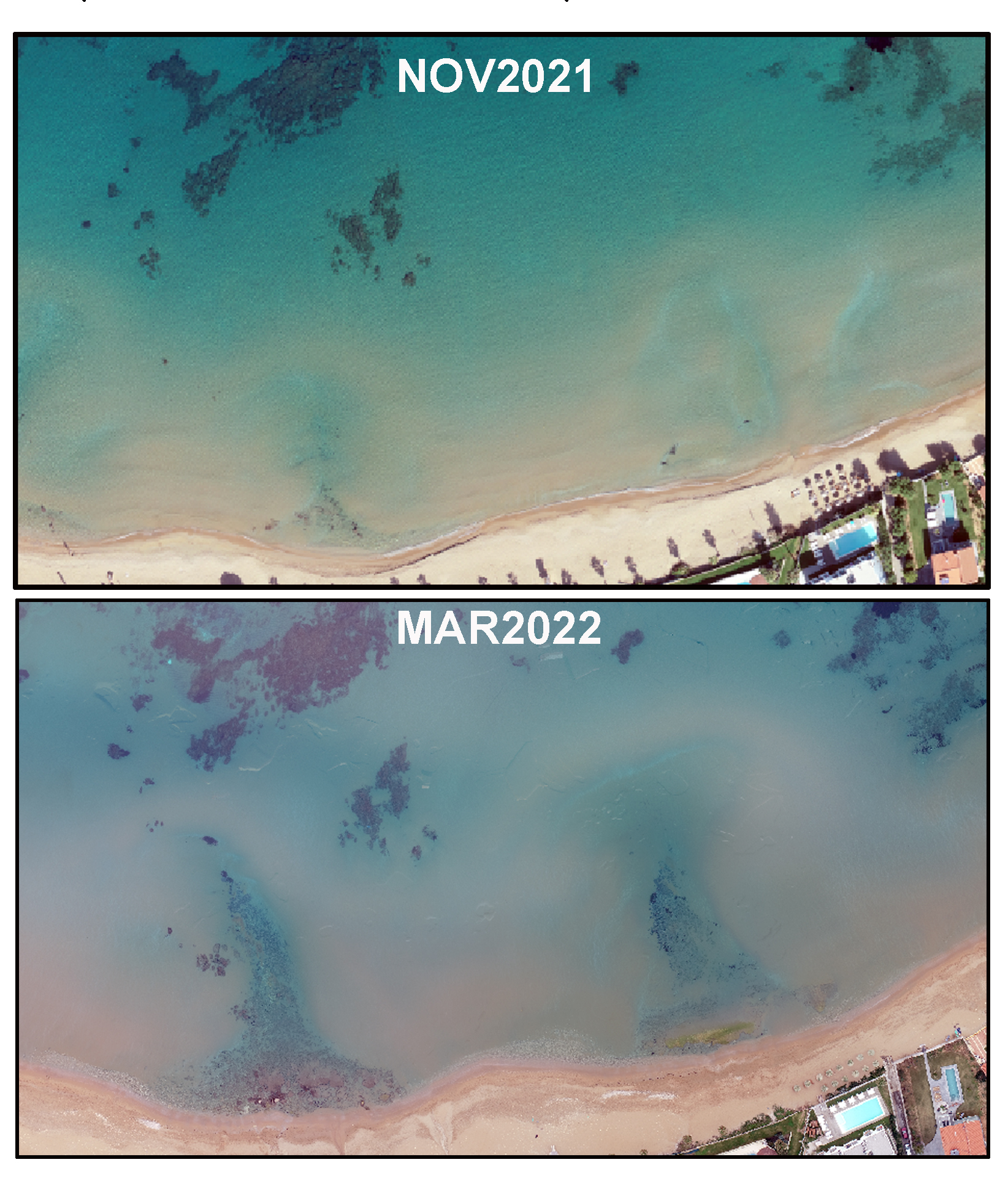
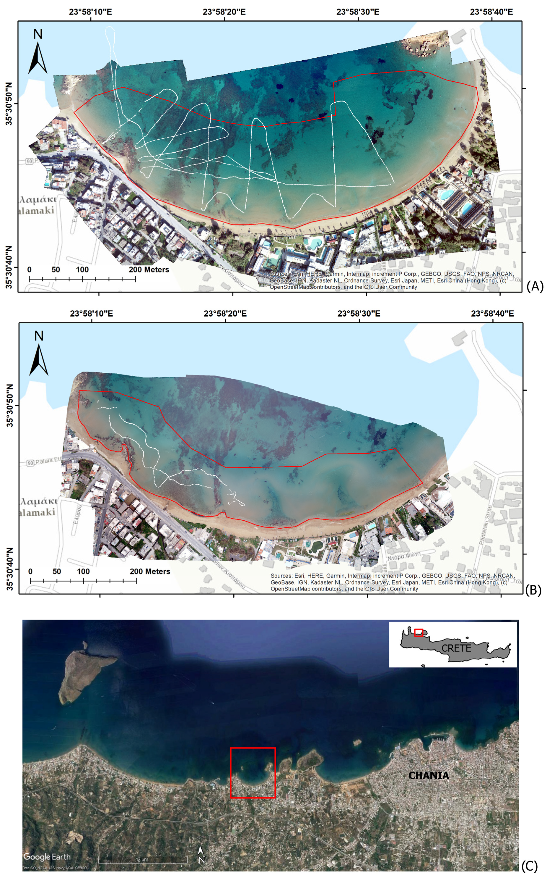
2.1. Study Area and Fieldwork

The wider study area (Figure 1) is located west of Chania city (Crete, Greece) and comprises of north-facing, sandy embayments with shallow, relatively smooth seafloor, covered with rocky reefs and exposed bedrock in places. The coastline in the Chania area stretches for at least 8 km and it is highly exposed to incoming waves from the north, which is the prevailing direction in the local wind regime [49], while significant along-shore sediment transport is expected due to incoming waves from various incidence angles [50]. The Chania area is characterized by increased water transparency due to low concentrations of chlorophyll (CHL-a) and suspended particulate matter (SPM), as a result of the oligotrophic character of the eastern Mediterranean Sea [51], and the absence of major input from adjacent drainage systems. A typical Secchi-depth for the study areas reaches at least ten meters. In addition, the average tidal range in Crete is at the scale of 10–20 cm.

Drone images were collected on 4 November 2021 and 31 March 2022, using a DJI Phantom 4 Pro drone. The drone was mounted with a 1-inch, 20-megapixel CMOS sensor and a MicaSense RedEgde-MX^© multispectral camera. Both sensors were set to collect images at nadir, with two-second intervals, along parallel flight tracks at 150 m altitude above sea level. Flying at high altitude assists in minimizing noise resulting from secondary reflections on the seafloor and on the sea surface. In order to avoid the sun glint effect on imagery, flights took place early in the morning when the sun elevation was lower than 30 degrees from horizon and the sea state was calm. Although the MS sensor records five spectral bands simultaneously (Blue, Green, Red, Red edge and Near infrared), in this study we only considered the Blue, Green and Red bands from the visible spectrum. These bands are more favorable in optical bathymetry studies [52,53], and their spectral characteristics are complementary with the built-in Red-Green-Blue (RGB) sensor of DJI Phantom 4 (Figure 2A;

Table A1. Spectral characteristics of standard RGB and multispectral bands used for building the composite 6-band cube. * full width at half maximum.

Band Name	Central Wavelength (nm)	Fwhm * (nm)
Blue	462	40
Green	525	50
Red	592	25
MS-Blue	480	10
MS-Green	560	10
MS-Red	671	5

, Appendix A). Depth measurements (Figure A1, Appendix A) were acquired on the same date as each drone survey, using an Ohmex BTX single-beam sonar with an operating frequency of 235 kHz. The sonar is integrated with a Real-Time Kinematics (RTK) GPS sensor for collecting attitude-corrected bathymetry points at 2 Hertz rate. The RTK-GPS measurements provide high spatial accuracy (<10 cm), which is essential in processing drone-based imagery with a pixel resolution of a few centimeters. The sonar were data acquired with a remotely controlled USV. The USV depth measurements were used for validating the outputs of bathymetry inversion by: (a) calculating the coefficient of determination (R²) as a measure of agreement between the sonar data and the predicted depth; (b) calculating the mean average error (MAE) and the root-mean-square error (RMSE) as metrics of the spread of the residuals; and (c) comparing the corresponding bathymetric profiles at each area.

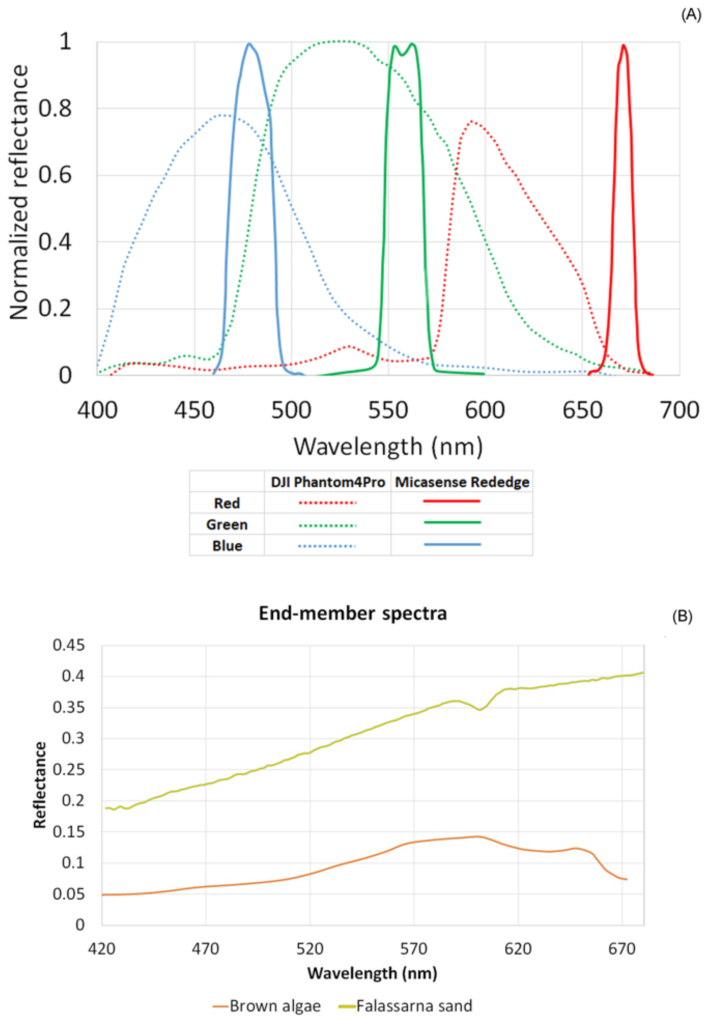
2.2. Pre-Processing of Drone-Based Imagery

The overall processing steps of drone images followed in this study are described in [54]. Initially, we produced one orthomosaic for each RGB and MS band (six in total) by applying RTK-GPS measurements of seven onshore ground-control points, and by performing the following radiometric and geometric corrections in Pix4D© software. Ref. [54] suggest that radiometric corrections of drone RGB imagery are required for improving shallow bathymetry results. Both RGB and MS images were adjusted for radial lens distortion using the respective camera models included in the Pix4D© software. The MS sensor was integrated with an external Downwelling Light Sensor (DLS-2) module, which records sun illumination parameters (i.e., angle, radiance) that are stored in the image metadata. These recordings are required during radiometric correction processing of multispectral imagery in Pix4D© software. In addition, the DLS-2 module provides GPS and attitude information for each acquired image, assisting the georeferencing and orthomosaicking of processed imagery using the Pix4D^© software. Initially, the pixel values are compensated for sensor bias such as sensor black-level, sensitivity, gain and exposure settings, and lens vignette effects, and then they are converted to radiance values (i.e., in units Wm⁻²sr⁻¹nm⁻¹, meaning watts per square meter per steradian per nanometer). Following this, the radiance values are converted to spectral reflectance for each band by incorporating the information from the reflectance panel and the DLS-2 sensor (available only for the MS images). In order to convert the pixel values to reflectance values, we acquired images of a spectral calibration panel which is specifically provided for the MS sensor and has a known reflectance coefficient for each band. The reference reflectance panel was also used for radiometric calibration of RGB images. A reference reflectance value of 0.51 was set for all bands (both RGB and MS), considering that this value accounts for all wavelengths in the visible spectrum (MicaSense©, personal communication by email, 3 November 2020). In this way, the final processed data are suitable for quantitative analysis. After the pre-processing stage, both RGB and MS reflectance orthomosaics were resampled at 15 cm pixel size and stacked together resulting in a six-band composite cube. The cube was converted to ENVI standard format for processing with the open-source WASI (WAtercolor SImulator) software. In this study, atmospheric correction of drone-based imagery was not performed. This is due to the fact that the drone surveys took place at significantly low altitude and with optimal weather conditions, thus atmospheric effects on recorded reflectance are minor. Following shallow water inversion (see next section) the output bathymetry maps were adjusted for tidal offsets by using tidal information from the Poseidon forecast website (“[55], https://poseidon.hcmr.gr/, accessed on 1 April 2022” n.d.).

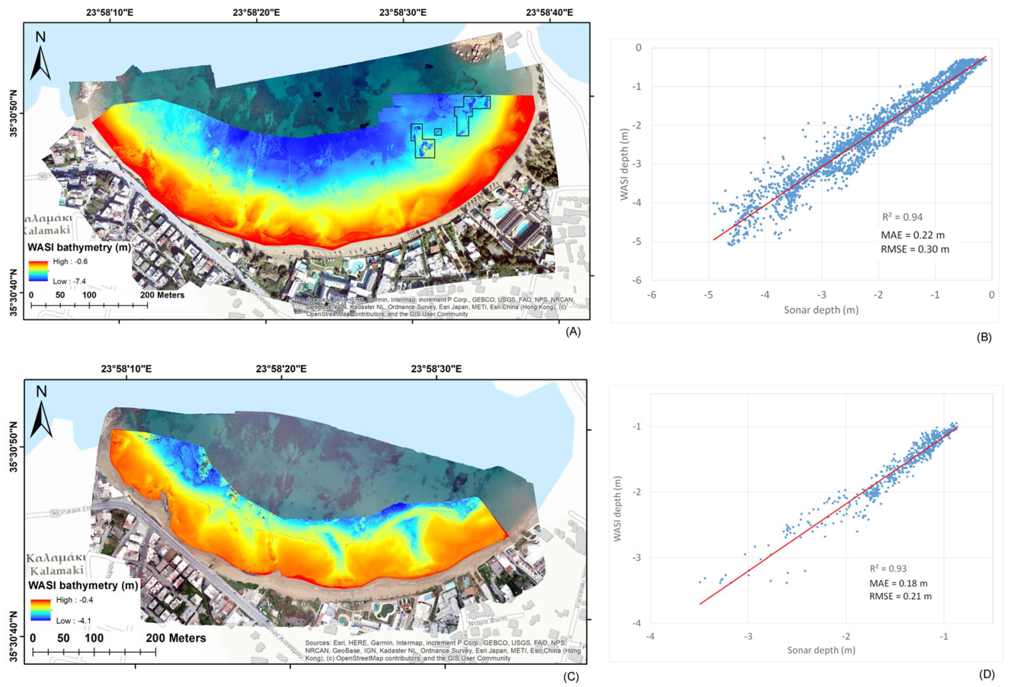
2.3. Shallow Bathymetry Inversion in WASI-2D

The WASI software is one of the few open-source tools for analyzing the spectral properties of aquatic environments. The WASI tool was initially designed for studying the water properties of fresh water environments, and it has been applied on a limited number of bathymetry studies, mainly in lake environments so far [56,57,58], while recently [59] applied WASI on PRISMA data from two Caribbean sites. The software is based on earlier bio-optical models developed by [52,60,61]. These models are applied on optically deep waters for estimating water-column constituents such as CHL-a and SPM, while they are also applied on optically shallow waters (i.e., where the influence of the seafloor is apparent) for deriving seafloor cover and water depth. WASI supports atmospherically corrected radiance and reflectance spectra, and it uses a down-welling irradiance model for estimating the effect of sun-glint and sky reflectance on the spectral signatures [57]. WASI includes a 2D module that allows for image analysis on a per-pixel basis [62]. This is particularly useful for analyzing imagery from multi- or hyper-spectral sensors. Regarding bathymetry retrieval, the WASI tool considers the influence of water-column constituents along with combinations of end-member seafloor reflectance spectra on water-leaving reflectances. For the current study we applied the end-member spectra of sand and brown algae (Figure 2B), which are more representative of the seafloor types that occur in our area than the default, end members provided by WASI. The sand spectrum was measured at Falassarna beach (50 km west of the study area) using a hand-held spectroradiometer (Alevizos and Alexakis, 2019, unpublished dataset). This type of sand consists of medium-sized, white grains with colored foraminifera fragments, which can be found in various coastal areas in the region of Chania. The brown algae spectrum was extracted from the project report of [63]. In their work, they measured underwater spectra using a spectroradiometer and a reference reflectance panel at various coastal locations in the southwest Indian Ocean. Suitable initial values of geometric (i.e., sun zenith angle) and irradiance model parameters are required for accurate fitting of the spectral signatures. Regarding datasets from both dates, we applied 0.1 mg/L for CHL-a and SPM concentrations and a sun zenith angle of 40 degrees. Ideally, in situ water column data should be applied for tuning these parameters; however, collecting such data was not practical in this study. Once the model is tuned, the depth and seafloor type are fitted using the least squares method iteratively. The modelled spectral signature showing the lowest residual with the observed signature is used to determine the depth and seafloor type for each pixel. A detailed description of the WASI tool can be found in [62]. The remote sensing reflectance in WASI is modelled according to the equations of [52,60]:

$$R_{rs}^{sh-}\left(\lambda \right)=R_{rs}^{deep-}\left(\lambda \right)\ast \left[1-A_{rs,1}\ast \exp \left\{-\left(K_d\left(\lambda \right)+K_{uW}\left(\lambda \right)\right)\ast Z_b\right\}\right]+A_{rs,2}\ast R_{rs}^b\left(\lambda \right)\ast \exp \left\{-\left(K_d\left(\lambda \right)+K_{u{\rm B}}\left(\lambda \right)\right)\ast Z_b\right\}$$

(1)

The superscript sh indicates shallow water, deep deep water, b bottom, and the symbol λ indicates the wavelength. The first term on the right-hand side is the contribution of water column with depth z_b, the second term represents the contribution of the bottom albedo. Light attenuation is described by the attenuation coefficients K_d for down-welling irradiance, Ku_W for upwelling radiance originating from the water layer, and K_uB for upwelling radiance from the bottom surface. These three coefficients are calculated as a function of the sun zenith angle, viewing direction and the concentrations of water constituents using equations also derived by [52,60]. A_rs,1 and A_rs,2 are empirical constants. The WASI algorithm iterates the spectral signatures on a per pixel basis, trying to fit an optimal spectrum given the constant values of model parameters. Inverse modeling takes place by approximating the remote sensing reflectance (Rrs) spectra (of each pixel) with suitable WASI spectra for different depths. The best fit with the observed image spectrum is obtained by minimizing a cost function that calculates the correlation between the Rrs and the WASI spectra. The inversion algorithm employs the absolute difference function in order to identify an optimal set of fit parameters (depth and seafloor type), which minimize the residual of the cost function [58,61,62].

3. Results

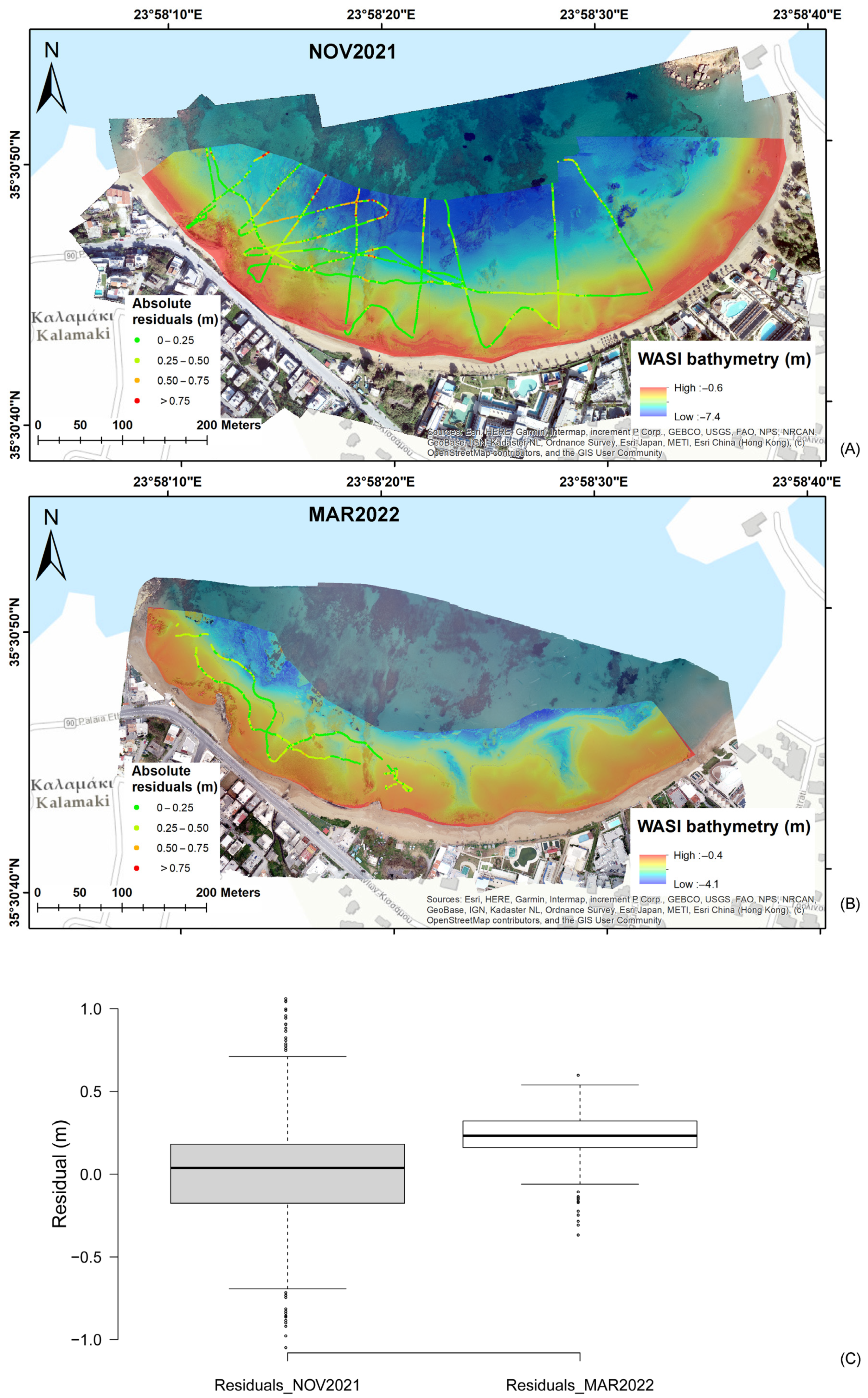
3.1. Bathymetry Validation

The bathymetry inversion outputs were validated with in situ sonar measurements from the USV platform. We compared the predicted versus the actual depth (tidally corrected) at each temporal dataset, and produced linear regression scatterplots from which the overall R², mean average error (MAE) and root-mean-square error (RMSE) were calculated as useful metrics for assessing the accuracy of each bathymetry dataset. The bathymetry inversion results show excellent agreement with in situ sonar measurements, and thus a temporal change analysis can be further performed. Specifically, the scatterplot for the November-2021 dataset (Figure 3B) shows optimal correspondence between the predicted and actual depths with R² = 0.94, and low error (MAE = 0.22 m; RMSE = 0.30 m). There are only a few instances of localized errors, and these are related to some seagrass patches, the depth of which was significantly overestimated by the WASI algorithm (Figure 3A). Regarding the March-2022 dataset, it shows a very good correlation coefficient between the predicted and the measured depth at R² = 0.93, and low error as well with MAE = 0.18 m and RMSE = 0.21 m (Figure 3D). We further examined the bathymetry residuals as per depth category (

Table 1. Descriptive statistics of bathymetry residuals per depth category.

4 November 21	0–1 m	1–2 m	2–3 m	3–4 m	4–5 m
Samples	498	573	597	423	177
MAE (m)	0.13	0.22	0.21	0.29	0.38
RMSE (m)	0.16	0.27	0.29	0.37	0.45
St.dev. (m)	0.16	0.26	0.28	0.35	0.40
31 March 22		1–2 m	2–3 m	3–4 m
Samples		434	113	14
MAE (m)		0.16	0.24	0.29
RMSE (m)		0.18	0.29	0.39
St.dev. (m)		0.10	0.19	0.30

). The residual statistics show a small increase in the error with increasing depth; however, this never exceeds 10% of the depth at each depth category. Figure 4 shows the spatial distribution of bathymetry residuals, providing further insight about the localized character of some outlier points. Regarding the data of November 2021, these points occur towards the deeper part of the area, and they are possibly related to abrupt changes in substrate. In March 2022 the residuals are lower, without any extreme outliers, and they have a 0.20 m bias. Box-plots in Figure 4C show that the majority (75%) of validation points have less than 0.30 m residual values, suggesting that the bathymetry maps are overall reliable for temporal change analysis.

The predicted bathymetry datasets show nearshore bedform features, matching those identified by [36] in the same area using high-resolution WorldView-3 imagery. These features appear somewhat clustered, forming a continuous “chain” along the coastline in the November-2021 bathymetry. In contrast, these features appear more interrupted in the March-2022 bathymetry dataset (Figure 3A,C).

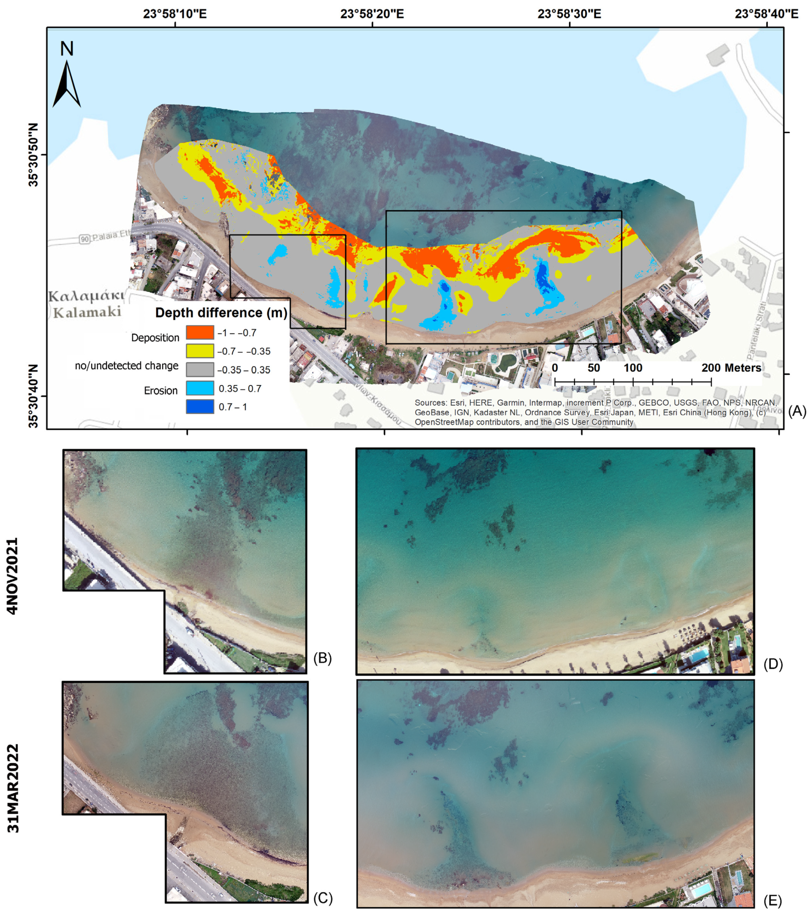
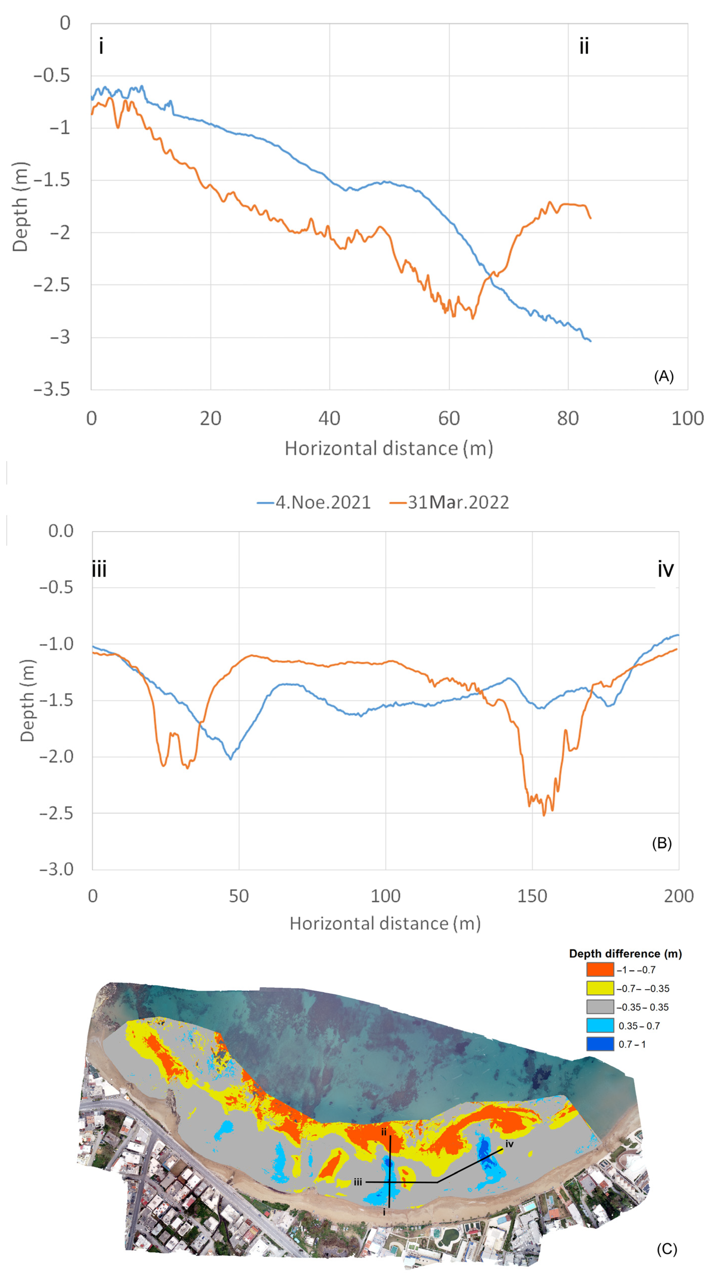
3.2. Short-Term Bathymetric Changes

The temporal drone imagery captured significant shallow seafloor changes that occurred within a five-month period. In order to facilitate a more objective comparison between the drone-based bathymetric datasets, we apply the combined RMSE metric that is the root of the squared sum of both RMSEs (November 2021 and March 2022). This metric suggests that bathymetric changes greater than the combined RMSE threshold of ±0.37 m are considered valid for a 68% confidence interval. Stark morphobathymetric changes are apparent, both on the RGB orthomosaics and on the differential bathymetry map (Figure 5). The differential bathymetry map was created by subtracting the March-2022 dataset from the November-2021 dataset (Figure 5A). In this way, we obtain a better idea of how bathymetry changed over this short period. The most prominent features on the bathymetric difference map are the development of two “channels” that are perpendicular to the coast (Figure 5E). They correspond to areas of intense erosion, resulting in uncovering of coarse seafloor sediments which are not apparent in the RGB orthomosaic of November-2021 dataset (Figure 5D). These features have an average width of 20 m, they are approximately 70 m long, and they are approximately 100 m apart. Further erosional features are observed in the west part of the scene close to a gravelly shoal (Figure 5B,C) where a larger portion of underlying seafloor is revealed in the March-2022 orthomosaics. A comparison of temporal bathymetric profiles, along and across these erosional features, shows 0.5–1 m difference within five months (Figure 6). Moreover, the along-shore profiles (Figure 6B) indicate that the rip channels are shifted ca. 25 m to the west, parallel to the shore, over the five-month period.

4. Discussion

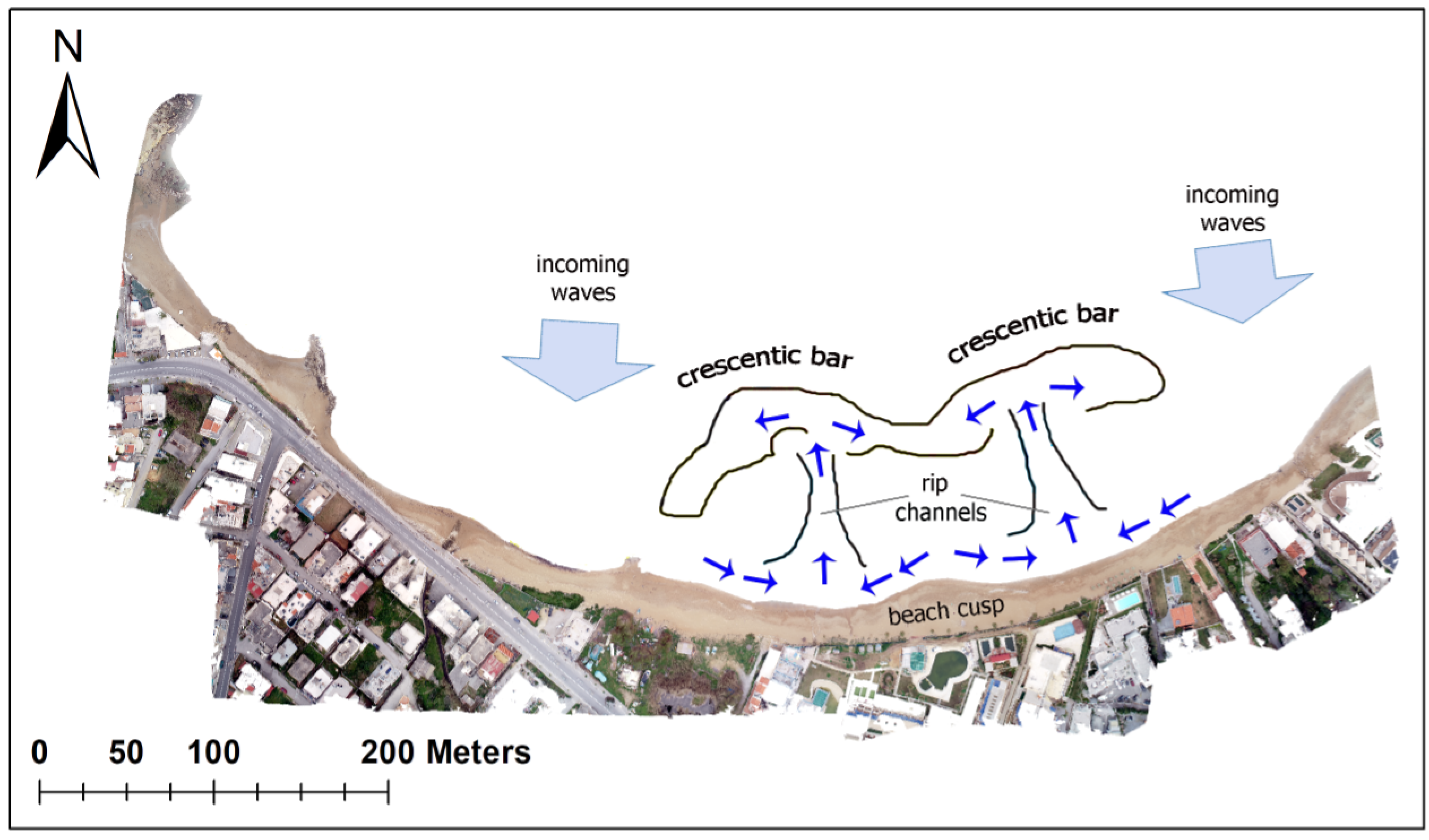
4.1. Interpretation of Nearshore Bathymetry Change

Change analysis between the temporal bathymetry datasets revealed geomorphological patterns that are typical for sandy coastal areas exposed to wave action from normal incidence angles [64,65]. These patterns are characterized as crescentic bar systems, and they are linked to processes that distribute large volume of sediments in the nearshore seafloor. Crescentic bars are apparent in both temporal RGB orthomosaics and bathymetry outputs (Figure 3 and Figure 5), and the bathymetry difference map highlights the paths of bar reorganization under the influence of enhanced wave and current activity during the winter months. Bathymetry data (Figure 3A,C) show that crescentic bars with secondary channel systems cover the entire nearshore part of the beach. Refs. [64,65] have reported that the development of the crescentic bar is linked to a self-organizing mechanism, which depends on the feedback between the seafloor geometry and the distribution of wave energy. Thus, we created a conceptual model representing coastal hydrodynamic activity based on the bathymetry difference map (Figure 7). The bathymetry difference map indicates two narrow corridors (rip channels) within which intense erosion occurred. The perpendicular orientation of the channels relative to the coastline suggests that the prevailing incidence angles of waves were directly from the north. This pattern of erosion process corresponds to rip-current action, which is part of the wider coastal cell circulation [66] (Figure 7). Rip channels are developed under the combination of wave focusing (due to refraction) and nearshore bathymetric variability [64,65]. The transported sediment is redeposited following the rhythmic pattern of the crescentic bar. Sediment deposition is controlled by the depth-averaged sediment concentration profiles [65]. Persistent rip-current action removes large volumes of sediments from the surf zone and deposits them further offshore [67], as shown in Figure 5E. Using the two bathymetric datasets, we estimated the volume of sediment that was eroded through the rip channels and found that more than 1500 cubic meters were removed during the 5-month period. The shape of nearshore bedforms is further controlled by the geometric characteristics of the beach (i.e., length) [68] and the occurrence of hard seafloor areas that influence sediment deposition.

It has been suggested that the crescentic bar oscillates between straight and crescentic form at various time scales, depending on the intensity and incidence angle of waves [69]. Usually a straight bar is developed during increased wave-energy events, while the crescentic bar is formed by a decrease in wave energy following these events [65]. When wave energy is increasing, the crescentic bar becomes straight again, through a process which is called a morphological reset [65]. Recent studies have shown that the crescentic bar is formed preferentially under normal wave incidence angles to the shore, while oblique wave angles lead mainly to morphological reset [68,70,71,72]. Such a behavior was not observed in the duration of the study. However, the crescentic bar appears to have migrated further offshore in the March-2022 bathymetry dataset, while in the November-2021 bathymetry dataset appears to be closer to the coastline. It is hypothesized that wave action during the winter storms resulted in dissociation of the “summer” structure of the bar, and a slow build-up of the deeper part of the bar as usually happens with typical beach profiles [73]. The only difference here is that this change occurs on a crescentic bar instead of a standard straight bar. This type of across-shore migration has also been reported in the studies of [48,67]. The bathymetric profile comparison in Figure 6 provides evidence that there is also a lateral migration of the crescentic bar (i.e., along shore). Drone-based bathymetry with high temporal resolution should assist in further understanding of the along-shore displacement of the crescentic bar.

4.2. Implications in Coastal Seafloor Monitoring

The presented study introduces a novel approach for monitoring small-scale nearshore seafloor change in areas with sufficient water transparency. This approach provides a robust alternative to LiDAR and multibeam surveying, for capturing fine-scale geomorphological features and short-term changes of shallow seafloor. The main advantage of this study is the effectiveness of multispectral imagery for mapping shallow bathymetry over seafloor consisting of loose sediments. Typically, drone imagery from such seafloor areas is not suitable for applying photogrammetric 3D reconstruction techniques since smooth seafloor does not hold enough texture. Consequently, multispectral data are required for overcoming this issue along with optical modelling. Although the drone-based bathymetry does not achieve the vertical accuracy of a multi-beam echo-sounder, it is considered sufficient for rapid bathymetry assessment and geomorphological mapping applications where area coverage is the primary goal. In this study, we exploited the effectiveness of a WASI shallow-water inversion model for producing bathymetry without utilizing input depth data. This is a very important aspect in shallow bathymetry mapping, where several studies rely on a large volume of in situ depth measurements for building accurate empirical models [9,30]. Obtaining extensive in situ data requires additional costs and logistical effort, which can be problematic for long-term bathymetry monitoring projects [34]. The presented study shows that radiometrically corrected, multispectral imagery from drones (with several bands in the visible range) is suitable for producing bathymetry outputs with significant detail. Thus, drone-based bathymetry provides a cost-effective approach that is suitable for shallow bathymetry change monitoring. Shallow water inversion models work well when imagery with suitable radiometric/atmospheric corrections is used, and when the model parameters (e.g., water-column constituents, end-member spectra) are representative of the study area. A particular advantage of drone imagery over satellite/airborne imagery regarding shallow water inversion is the fact that the first does not require atmospheric correction. The atmospheric effects on drone-based imagery are considered minor for bright targets in the visible spectrum, and when images are taken from less than 150 m altitude under favorable weather conditions [74]. However, the use of a calibration reflectance panel is required for obtaining reflectance values adjusted for incoming radiance. Regarding water-column and seafloor spectra data for model tuning, this information can be extracted from various sources. Information about the concertation of water-column constituents according to water-type is found in current literature, and can be retrieved from large-scale satellite products (e.g., CHL-a and SPM from Copernicus missions). Seafloor end-member spectra covering various locations (e.g., temperate, tropical) have been published as well, providing a useful alternative to collecting these data in situ [63]. These studies were based on the method of [41] about integrating RGB and MS data into a single image-cube. Thus, we recommend that a standard type of MS sensor and data pre-processing should be developed in the future, targeting particularly shallow bathymetry applications. A potential sensor for drone-based bathymetry mapping should comprise at least five narrow spectral bands spanning in the visible range. Five spectral bands are considered to provide an acceptable radiometric resolution that is required for shallow bathymetry inversion [29,53,75]. Additionally, a dedicated radiometric calibration procedure should be implemented for this particular type of sensor in order to convert pixel values to reflectance. The availability of such a sensor would enable a wider variety of shallow seafloor mapping applications to be realized. Particularly, high temporal resolution bathymetry datasets will allow us to visualize better the geometric and migration characteristics of rip channel systems, and thus assist in a better understanding of nearshore seafloor change. Drone-based bathymetry is expected to cover a significant gap in coastal modelling studies [76], and act synergistically with other in situ methods (i.e., GPS drifters) for improving the knowledge about nearshore features and processes.

4.3. Sources of Error and Method Limitations

The presented datasets and methods show promising results in shallow seafloor geomorphological mapping. However, there are some points where particular attention is required in order to avoid or minimize potential sources of error. Drone imagery is usually prone to lower signal-to-noise (S/N) ratio compared to satellite imagery [77], due to image noise related to sun glint, wave-focusing or shadowing. Thus, specific requirements should be met for RGB and multispectral image acquisition and processing. In order to improve the S/N ratio it is suggested that drone imagery is acquired at low sun elevation angles (<30 degrees) [78]. When the sun is closer to the horizon, sun-glint and unwanted reflections are minimized and seafloor albedo is more uniform. In case that image noise is present, then image-filtering methods should be applied in post-processing. The simplest approach is to resample the imagery at greater pixel size so that noise is suppressed, and reflectance values are more homogenous. Another potential limitation is the maximum depth for applying optical models for inversion. In general, bathymetry inversion using radiative-transfer models works better for depths up to 10 m [30] with vertical errors increasing beyond this value. The main reason behind this behavior is related to the very low, water-leaving reflectance values that introduce spectral matching problems during inversion [30,77].

5. Conclusions

The application of shallow bathymetry inversion on drone-based imagery provided an efficient approach for mapping nearshore geomorphological features and short-term bathymetric changes at a small sandy bay in Greece. A composite image cube with increased spectral resolution in the visible spectrum resulted from the combination of radiometrically corrected drone-based RGB and MS orthomosaics used for bathymetry inversion. Predicted bathymetry showed <0.3 m average vertical errors when compared with USV sonar bathymetry. Nearshore bedforms identified on drone-based temporal bathymetry datasets are characterized as crescentic bars and rip channel systems. Evidence on differential bathymetry and true-color orthomosaics suggests that two main rip channels developed during a period of five months, driven by the impact of wave action in winter. Temporal bathymetric profiles suggest that the crescentic bar system transforms from summer to winter geometry and migrates along-shore at a short-term time-scale. In general, the drone-based bathymetry assisted in capturing the geographic boundaries of local hydrodynamic patterns. Future improvements in drone sensors are expected to lead to a greater variety of shallow bathymetry applications.

References

1. Davidson, M.; Van Koningsveld, M.; de Kruif, A.; Rawson, J.; Holman, R.; Lamberti, A.; Medina, R.; Kroon, A.; Aarninkhof, S. The CoastView Project: Developing Video-Derived Coastal State Indicators in Support of Coastal Zone Management. Coast. Eng. 2007, 54, 463–475. [Google Scholar] [CrossRef]
2. de Swart, H.E.; Zimmerman, J.T.F. Morphodynamics of Tidal Inlet Systems. Annu. Rev. Fluid Mech. 2009, 41, 203–229. [Google Scholar] [CrossRef]
3. van Dongeren, A.; Plant, N.; Cohen, A.; Roelvink, D.; Haller, M.C.; Catalán, P. Beach Wizard: Nearshore Bathymetry Estimation through Assimilation of Model Computations and Remote Observations. Coast. Eng. 2008, 55, 1016–1027. [Google Scholar] [CrossRef]
4. Jackson, D.W.T.; Short, A.D.; Loureiro, C.; Cooper, J.A.G. Beach Morphodynamic Classification Using High-Resolution Nearshore Bathymetry and Process-Based Wave Modelling. Estuar. Coast. Shelf Sci. 2022, 268, 107812. [Google Scholar] [CrossRef]
5. Misra, A.; Ramakrishnan, B. Assessment of Coastal Geomorphological Changes Using Multi-Temporal Satellite-Derived Bathymetry. Cont. Shelf Res. 2020, 207, 104213. [Google Scholar] [CrossRef]
6. Toodesh, R.; Verhagen, S.; Dagla, A. Prediction of Changes in Seafloor Depths Based on Time Series of Bathymetry Observations: Dutch North Sea Case. J. Mar. Sci. Eng. 2021, 9, 931. [Google Scholar] [CrossRef]
7. Agrafiotis, P.; Karantzalos, K.; Georgopoulos, A.; Skarlatos, D. Correcting Image Refraction: Towards Accurate Aerial Image-Based Bathymetry Mapping in Shallow Waters. Remote Sens. 2020, 12, 322. [Google Scholar] [CrossRef] [Green Version]
8. Gao, J. Bathymetric Mapping by Means of Remote Sensing: Methods, Accuracy and Limitations. Prog. Phys. Geogr. Earth Environ. 2009, 33, 103–116. [Google Scholar] [CrossRef]
9. Salameh, E.; Frappart, F.; Almar, R.; Baptista, P.; Heygster, G.; Lubac, B.; Raucoules, D.; Almeida, L.P.; Bergsma, E.W.J.; Capo, S.; et al. Monitoring Beach Topography and Nearshore Bathymetry Using Spaceborne Remote Sensing: A Review. Remote Sens. 2019, 11, 2212. [Google Scholar] [CrossRef] [Green Version]
10. Lee, Z.; Casey, B.; Arnone, R.A.; Weidemann, A.D.; Parsons, R.; Montes, M.J.; Gao, B.-C.; Goode, W.; Davis, C.O.; Dye, J. Water and Bottom Properties of a Coastal Environment Derived from Hyperion Data Measured from the EO-1 Spacecraft Platform. J. Appl. Remote Sens. 2007, 1, 011502. [Google Scholar] [CrossRef]
11. Bergsma, E.W.J.; Almar, R. Video-Based Depth Inversion Techniques, a Method Comparison with Synthetic Cases. Coast. Eng. 2018, 138, 199–209. [Google Scholar] [CrossRef]
12. Collins, A.M.; Geheran, M.P.; Hesser, T.J.; Bak, A.S.; Brodie, K.L.; Farthing, M.W. Development of a Fully Convolutional Neural Network to Derive Surf-Zone Bathymetry from Close-Range Imagery of Waves in Duck, NC. Remote Sens. 2021, 13, 4907. [Google Scholar] [CrossRef]
13. Costa, B.M.; Battista, T.A.; Pittman, S.J. Comparative Evaluation of Airborne LiDAR and Ship-Based Multibeam SoNAR Bathymetry and Intensity for Mapping Coral Reef Ecosystems. Remote Sens. Environ. 2009, 113, 1082–1100. [Google Scholar] [CrossRef]
14. Janowski, L.; Wroblewski, R.; Rucinska, M.; Kubowicz-Grajewska, A.; Tysiac, P. Automatic Classification and Mapping of the Seabed Using Airborne LiDAR Bathymetry. Eng. Geol. 2022, 301, 106615. [Google Scholar] [CrossRef]
15. Klemas, V. Beach Profiling and LIDAR Bathymetry: An Overview with Case Studies. J. Coast. Res. 2011, 277, 1019–1028. [Google Scholar] [CrossRef]
16. Taramelli, A.; Cappucci, S.; Valentini, E.; Rossi, L.; Lisi, I. Nearshore Sandbar Classification of Sabaudia (Italy) with LiDAR Data: The FHyL Approach. Remote Sens. 2020, 12, 1053. [Google Scholar] [CrossRef] [Green Version]
17. Brock, J.C.; Purkis, S.J. The Emerging Role of Lidar Remote Sensing in Coastal Research and Resource Management. J. Coast. Res. 2009, 53, 1–5. [Google Scholar] [CrossRef]
18. Freire, R.; Pe’eri, S.; Madore, B.; Rzhanov, Y.; Alexander, L.; Parrish, C.; Lippmann, T. Monitoring Near-Shore Bathymetry Using a Multi-Image Satellite-Derived Bathymetry Approach. In Proceedings of the US Hydrographic Conference 2015, National Harbor, MD, USA, 16–19 March 2015. [Google Scholar]
19. Lyzenga, D.R. Passive Remote Sensing Techniques for Mapping Water Depth and Bottom Features. Appl. Opt. 1978, 17, 379–383. [Google Scholar] [CrossRef] [PubMed]
20. Stumpf, R.P.; Holderied, K.; Sinclair, M. Determination of Water Depth with High-Resolution Satellite Imagery over Variable Bottom Types. Limnol. Oceanogr. 2003, 48, 547–556. [Google Scholar] [CrossRef]
21. Geyman, E.C.; Maloof, A.C. A Simple Method for Extracting Water Depth from Multispectral Satellite Imagery in Regions of Variable Bottom Type. Earth Space Sci. 2019, 6, 527–537. [Google Scholar] [CrossRef]
22. Gholamalifard, M.; Kutser, T.; Esmaili-Sari, A.; Abkar, A.A.; Naimi, B. Remotely Sensed Empirical Modeling of Bathymetry in the Southeastern Caspian Sea. Remote Sens. 2013, 5, 2746–2762. [Google Scholar] [CrossRef] [Green Version]
23. Ma, S.; Tao, Z.; Yang, X.; Yu, Y.; Zhou, X.; Li, Z. Bathymetry Retrieval from Hyperspectral Remote Sensing Data in Optical-Shallow Water. IEEE Trans. Geosci. Remote Sens. 2014, 52, 1205–1212. [Google Scholar] [CrossRef]
24. Traganos, D.; Poursanidis, D.; Aggarwal, B.; Chrysoulakis, N.; Reinartz, P. Estimating Satellite-Derived Bathymetry (SDB) with the Google Earth Engine and Sentinel-2. Remote Sens. 2018, 10, 859. [Google Scholar] [CrossRef] [Green Version]
25. Wei, C.; Zhao, Q.; Lu, Y.; Fu, D. Assessment of Empirical Algorithms for Shallow Water Bathymetry Using Multi-Spectral Imagery of Pearl River Delta Coast, China. Remote Sens. 2021, 13, 3123. [Google Scholar] [CrossRef]
26. Kibele, J.; Shears, N.T. Nonparametric Empirical Depth Regression for Bathymetric Mapping in Coastal Waters. IEEE J. Sel. Top. Appl. Earth Obs. Remote Sens. 2016, 9, 5130–5138. [Google Scholar] [CrossRef]
27. Caballero, I.; Stumpf, R.P. Retrieval of Nearshore Bathymetry from Sentinel-2A and 2B Satellites in South Florida Coastal Waters. Estuar. Coast. Shelf Sci. 2019, 226, 106277. [Google Scholar] [CrossRef]
28. Dekker, A.G.; Phinn, S.R.; Anstee, J.; Bissett, P.; Brando, V.E.; Casey, B.; Fearns, P.; Hedley, J.; Klonowski, W.; Lee, Z.P.; et al. Intercomparison of Shallow Water Bathymetry, Hydro-Optics, and Benthos Mapping Techniques in Australian and Caribbean Coastal Environments. Limnol. Oceanogr. Methods 2011, 9, 396–425. [Google Scholar] [CrossRef] [Green Version]
29. Klonowski, W.M. Retrieving Key Benthic Cover Types and Bathymetry from Hyperspectral Imagery. J. Appl. Remote Sens. 2007, 1, 011505. [Google Scholar] [CrossRef]
30. Kutser, T.; Hedley, J.; Giardino, C.; Roelfsema, C.; Brando, V.E. Remote Sensing of Shallow Waters—A 50 Year Retrospective and Future Directions. Remote Sens. Environ. 2020, 240, 111619. [Google Scholar] [CrossRef]
31. Leiper, I.A.; Phinn, S.R.; Roelfsema, C.M.; Joyce, K.E.; Dekker, A.G. Mapping Coral Reef Benthos, Substrates, and Bathymetry, Using Compact Airborne Spectrographic Imager (CASI) Data. Remote Sens. 2014, 6, 6423–6445. [Google Scholar] [CrossRef]
32. Lee, Z.; Carder, K.L.; Mobley, C.D.; Steward, R.G.; Patch, J.S. Hyperspectral Remote Sensing for Shallow Waters: 2. Deriving Bottom Depths and Water Properties by Optimization. Appl. Opt. 1999, 38, 3831–3843. [Google Scholar] [CrossRef] [PubMed] [Green Version]
33. Mobley, C.D.; Sundman, L.K.; Davis, C.O.; Bowles, J.H.; Downes, T.V.; Leathers, R.A.; Montes, M.J.; Bissett, W.P.; Kohler, D.D.R.; Reid, R.P.; et al. Interpretation of Hyperspectral Remote-Sensing Imagery by Spectrum Matching and Look-up Tables. Appl. Opt. 2005, 44, 3576–3592. [Google Scholar] [CrossRef] [PubMed]
34. Capo, S.; Lubac, B.; Marieu, V.; Robinet, A.; Bru, D.; Bonneton, P. Assessment of the Decadal Morphodynamic Evolution of a Mixed Energy Inlet Using Ocean Color Remote Sensing. Ocean Dyn. 2014, 64, 1517–1530. [Google Scholar] [CrossRef]
35. Bolaños, R.; Hansen, L.B.; Rasmussen, M.L.; Golestani, M.; Mariegaard, J.S.; Nielsen, L.T. Coastal Bathymetry from Satellite and Its Use on Coastal Modelling. Coast. Eng. Proc. 2018, 1, 98. [Google Scholar] [CrossRef] [Green Version]
36. Alevizos, E.; Roussos, A.; Alexakis, D. Geomorphometric Analysis of Nearshore Sedimentary Bedforms from High-Resolution Multi-Temporal Satellite-Derived Bathymetry. Geocarto Int. 2021, 1–17. [Google Scholar] [CrossRef]
37. Pacheco, A.; Horta, J.; Loureiro, C.; Ferreira, Ó. Retrieval of Nearshore Bathymetry from Landsat 8 Images: A Tool for Coastal Monitoring in Shallow Waters. Remote Sens. Environ. 2015, 159, 102–116. [Google Scholar] [CrossRef] [Green Version]
38. Alevizos, E. How to Create High Resolution Digital Elevation Models of Terrestrial Landscape Using Uav Imagery and Open-Source Software; Research Gate: Berlin, Germany, 2019. [Google Scholar] [CrossRef]
39. Román, A.; Tovar-Sánchez, A.; Olivé, I.; Navarro, G. Using a UAV-Mounted Multispectral Camera for the Monitoring of Marine Macrophytes. Front. Mar. Sci. 2021, 8, 722698. [Google Scholar] [CrossRef]
40. Rossi, L.; Mammi, I.; Pelliccia, F. UAV-Derived Multispectral Bathymetry. Remote Sens. 2020, 12, 3897. [Google Scholar] [CrossRef]
41. Alevizos, E.; Oikonomou, D.; Argyriou, A.V.; Alexakis, D.D. Fusion of Drone-Based RGB and Multi-Spectral Imagery for Shallow Water Bathymetry Inversion. Remote Sens. 2022, 14, 1127. [Google Scholar] [CrossRef]
42. Kabiri, K.; Rezai, H.; Moradi, M. A Drone-Based Method for Mapping the Coral Reefs in the Shallow Coastal Waters—Case Study: Kish Island, Persian Gulf. Earth Sci. Inform. 2020, 13, 1265–1274. [Google Scholar] [CrossRef]
43. Parsons, M.; Bratanov, D.; Gaston, K.; Gonzalez, F. UAVs, Hyperspectral Remote Sensing, and Machine Learning Revolutionizing Reef Monitoring. Sensors 2018, 18, 2026. [Google Scholar] [CrossRef] [Green Version]
44. Slocum, R.K.; Parrish, C.E.; Simpson, C.H. Combined Geometric-Radiometric and Neural Network Approach to Shallow Bathymetric Mapping with UAS Imagery. ISPRS J. Photogramm. Remote Sens. 2020, 169, 351–363. [Google Scholar] [CrossRef]
45. Starek, M.J.; Giessel, J. Fusion of Uas-Based Structure-from-Motion and Optical Inversion for Seamless Topo-Bathymetric Mapping. In Proceedings of the 2017 IEEE International Geoscience and Remote Sensing Symposium (IGARSS), Fort Worth, TX, USA, 23–28 July 2017; pp. 2999–3002. [Google Scholar]
46. Agrafiotis, P.; Skarlatos, D.; Georgopoulos, A.; Karantzalos, K. Shallow water bathymetry mapping from uav imagery based on machine learning. ISPRS Int. Arch. Photogramm. Remote Sens. Spat. Inf. Sci. 2019, XLII-2/W10, 9–16. [Google Scholar] [CrossRef] [Green Version]
47. Dietrich, J.T. Bathymetric Structure-from-Motion: Extracting Shallow Stream Bathymetry from Multi-View Stereo Photogrammetry. Earth Surf. Process. Landf. 2017, 42, 355–364. [Google Scholar] [CrossRef]
48. Biausque, M.; Guisado-Pintado, E.; Grottoli, E.; Jackson, D.W.T.; Cooper, J.A.G. Seasonal Morphodynamics of Multiple Intertidal Bars (MITBs) on a Meso- to Macrotidal Beach. Earth Surf. Process. Landf. 2022, 47, 839–853. [Google Scholar] [CrossRef]
49. Foteinis, S.; Synolakis, C.; Tsoutsos, T. Numerical Modelling for Coastal Structures Design and Planning. A Case Study of the Venetian Harbour of Chania, Greece. Int. J. Geoengin. Case Hist 2018, 4, 232. [Google Scholar] [CrossRef]
50. Tsoukala, V.K.; Katsardi, V.; Hadjibiros, K.; Moutzouris, C.I. Beach Erosion and Consequential Impacts Due to the Presence of Harbours in Sandy Beaches in Greece and Cyprus. Environ. Process. 2015, 2, 55–71. [Google Scholar] [CrossRef] [Green Version]
51. Ignatiades, L. The Productive and Optical Status of the Oligotrophic Waters of the Southern Aegean Sea (Cretan Sea), Eastern Mediterranean. J. Plankton Res. 1998, 20, 985–995. [Google Scholar] [CrossRef]
52. Albert, A. Inversion Technique for Optical Remote Sensing in Shallow Water. Optische Fernerkundung von Flachwasserzonen. Ph.D. Thesis, University of Hamburg, Hamburg, Germany, 2004. [Google Scholar]
53. Marcello, J.; Eugenio, F.; Martín, J.; Marqués, F. Seabed Mapping in Coastal Shallow Waters Using High Resolution Multispectral and Hyperspectral Imagery. Remote Sens. 2018, 10, 1208. [Google Scholar] [CrossRef]
54. Alevizos, E.; Alexakis, D.D. Evaluation of Radiometric Calibration of Drone-Based Imagery for Improving Shallow Bathymetry Retrieval. Remote Sens. Lett. 2022, 13, 311–321. [Google Scholar] [CrossRef]
55. Poseidon System. Available online: https://poseidon.hcmr.gr/ (accessed on 1 April 2022).
56. Gege, P. A Case Study at Starnberger See for Hyperspectral Bathymetry Mapping Using Inverse Modeling. In Proceedings of the 2014 6th Workshop on Hyperspectral Image and Signal Processing: Evolution in Remote Sensing (WHISPERS), Lausanne, Switzerland, 24–27 June 2014; pp. 1–4. [Google Scholar]
57. Dörnhöfer, K.; Göritz, A.; Gege, P.; Pflug, B.; Oppelt, N. Water Constituents and Water Depth Retrieval from Sentinel-2A—A First Evaluation in an Oligotrophic Lake. Remote Sens. 2016, 8, 941. [Google Scholar] [CrossRef] [Green Version]
58. Niroumand-Jadidi, M.; Bovolo, F.; Bruzzone, L.; Gege, P. Physics-Based Bathymetry and Water Quality Retrieval Using PlanetScope Imagery: Impacts of 2020 COVID-19 Lockdown and 2019 Extreme Flood in the Venice Lagoon. Remote Sens. 2020, 12, 2381. [Google Scholar] [CrossRef]
59. Alevizos, E.; Le Bas, T.; Alexakis, D. Assessment of PRISMA Level-2 Hyperspectral Imagery for Large Scale Satellite-Derived Bathymetry Retrieval. Mar. Geod. 2022, 45, 251–273. [Google Scholar] [CrossRef]
60. Albert, A.; Mobley, C.D. An Analytical Model for Subsurface Irradiance and Remote Sensing Reflectance in Deep and Shallow Case-2 Waters. Opt. Express 2003, 11, 2873–2890. [Google Scholar] [CrossRef] [PubMed]
61. Gege, P.; Albert, A. A tool for inverse modeling of spectral measurements in deep and shallow waters. In Remote Sensing of Aquatic Coastal Ecosystem Processes; Remote Sensing and Digital Image Processing; Richardson, L.L., Ledrew, E.F., Eds.; Springer: Dordrecht, The Netherlands, 2006; pp. 81–109. ISBN 978-1-4020-3968-3. [Google Scholar]
62. Gege, P. WASI-2D: A Software Tool for Regionally Optimized Analysis of Imaging Spectrometer Data from Deep and Shallow Waters. Comput. Geosci. 2014, 62, 208–215. [Google Scholar] [CrossRef] [Green Version]
63. Mouquet, P.; Quod, J.-P. Spectrhabent-OI-Acquisition et Analyse de la Librairie Spectrale Sous-Marine; Archimer: Plouzane, France, 2010. [Google Scholar]
64. Castelle, B.; Ruessink, B.G.; Bonneton, P.; Marieu, V.; Bruneau, N.; Price, T.D. Coupling Mechanisms in Double Sandbar Systems. Part 1: Patterns and Physical Explanation. Earth Surf. Process. Landf. 2010, 35, 476–486. [Google Scholar] [CrossRef]
65. Ribas, F.; Falqués, A.; de Swart, H.E.; Dodd, N.; Garnier, R.; Calvete, D. Understanding Coastal Morphodynamic Patterns from Depth-Averaged Sediment Concentration. Rev. Geophys. 2015, 53, 362–410. [Google Scholar] [CrossRef] [Green Version]
66. Castelle, B.; Scott, T.; Brander, R.W.; McCarroll, R.J. Rip Current Types, Circulation and Hazard. Earth-Sci. Rev. 2016, 163, 1–21. [Google Scholar] [CrossRef]
67. Andreeva, N.; Saprykina, Y.; Valchev, N.; Eftimova, P.; Kuznetsov, S. Influence of Wave Climate on Intra and Inter-Annual Nearshore Bar Dynamics for a Sandy Beach. Geosciences 2021, 11, 206. [Google Scholar] [CrossRef]
68. Holman, R.A.; Symonds, G.; Thornton, E.B.; Ranasinghe, R. Rip Spacing and Persistence on an Embayed Beach. J. Geophys. Res. Oceans 2006, 111, C01006. [Google Scholar] [CrossRef] [Green Version]
69. Garnier, R.; Falqués, A.; Calvete, D.; Thiébot, J.; Ribas, F. A Mechanism for Sandbar Straightening by Oblique Wave Incidence. Geophys. Res. Lett. 2013, 40, 2726–2730. [Google Scholar] [CrossRef] [Green Version]
70. Price, T.D.; Ruessink, B.G. State Dynamics of a Double Sandbar System. Cont. Shelf Res. 2011, 31, 659–674. [Google Scholar] [CrossRef]
71. Splinter, K.D.; Holman, R.A.; Plant, N.G. A Behavior-Oriented Dynamic Model for Sandbar Migration and 2DH Evolution. J. Geophys. Res. Oceans 2011, 116, C01020. [Google Scholar] [CrossRef] [Green Version]
72. Thornton, E.B.; MacMahan, J.; Sallenger, A.H. Rip Currents, Mega-Cusps, and Eroding Dunes. Mar. Geol. 2007, 240, 151–167. [Google Scholar] [CrossRef]
73. Dean, R. Equilibrium Beach Profiles: Characteristics and Applications. J. Coast. Res. 1991, 7, 53–84. [Google Scholar]
74. Suomalainen, J.; Oliveira, R.A.; Hakala, T.; Koivumäki, N.; Markelin, L.; Näsi, R.; Honkavaara, E. Direct Reflectance Transformation Methodology for Drone-Based Hyperspectral Imaging. Remote Sens. Environ. 2021, 266, 112691. [Google Scholar] [CrossRef]
75. Hedley, J.D.; Roelfsema, C.; Brando, V.; Giardino, C.; Kutser, T.; Phinn, S.; Mumby, P.J.; Barrilero, O.; Laporte, J.; Koetz, B. Coral Reef Applications of Sentinel-2: Coverage, Characteristics, Bathymetry and Benthic Mapping with Comparison to Landsat 8. Remote Sens. Environ. 2018, 216, 598–614. [Google Scholar] [CrossRef]
76. Holman, R.; Haller, M.C. Remote Sensing of the Nearshore. Annu. Rev. Mar. Sci. 2013, 5, 95–113. [Google Scholar] [CrossRef] [Green Version]
77. Dierssen, H.M.; Ackleson, S.G.; Joyce, K.E.; Hestir, E.L.; Castagna, A.; Lavender, S.; McManus, M.A. Living up to the Hype of Hyperspectral Aquatic Remote Sensing: Science, Resources and Outlook. Front. Environ. Sci. 2021, 9, 649528. [Google Scholar] [CrossRef]
78. Hovis, W.A.; Clark, D.K.; Anderson, F.; Austin, R.W.; Wilson, W.H.; Baker, E.T.; Ball, D.; Gordon, H.R.; Mueller, J.L.; El-Sayed, S.Z.; et al. Nimbus-7 Coastal Zone Color Scanner: System Description and Initial Imagery. Science 1980, 210, 60–63. [Google Scholar] [CrossRef]
Figure 1. Temporal, true-color orthomosaics of the study area: (A) Imagery acquired on 4 November 2021; (B) Imagery acquired on 31 March 2022; (C) Legend map of the wider study area. The red rectangles show the processing boundaries of bathymetry inversion, and the white dots correspond to the track of USV sonar measurements.
Remotesensing 14 06035 g001
Figure 2. (A) Spectral responses of both RGB and MS sensors (Source: [41]); (B) Spectral signatures of the two end-member spectra used for bathymetry inversion.
Remotesensing 14 06035 g002
Figure 3. (A) Bathymetry inversion output for the November-2021 dataset. Black polygons indicate erroneous results due to the presence of seagrass patches; (B) Linear regression between modelled and measured depth for the November-2021 datasets; (C) Bathymetry inversion output for the March-2022 dataset; (D) Linear regression between modelled and measured depth for the March-2022 datasets. The red line in the regression plots indicates the linear trend of the correlation.
Remotesensing 14 06035 g003
Figure 4. Absolute residual values over bathymetry map for: (A) November 2021 bathymetry inversion; (B) March 2022 bathymetry inversion; (C) Box-plots of residual values for each date. The black horizontal line inside each box indicates the median value of each sample and the whiskers extend from the 1st to the 3rd quartile.
Remotesensing 14 06035 g004
Figure 5. (A) Bathymetric difference map (November-2021 minus March-2022); (B,C) True-color orthomosaic subsets showing the temporal changes within the left polygon area; (D,E) True-color orthomosaic subsets showing the temporal changes within the right rectangle area.
Remotesensing 14 06035 g005
Figure 6. Temporal bathymetric profiles: (A) across-shore (i–ii); and (B) along-shore (iii–iv); (C) Legend map showing the profiles on the bathymetry difference map.
Remotesensing 14 06035 g006
Figure 7. Conceptual model about coastal circulation and corresponding geomorphology features occurring at the study area. This model resulted from an adaptation of the bathymetric difference map (Figure 5). The thin blue arrows indicate the direction of nearshore currents.
Remotesensing 14 06035 g007