Article

Predicting the Forest Canopy Height from LiDAR and Multi-Sensor Data Using Machine Learning over India

1
Solid World DAO, Pärnu mnt 15 // Tatari tn 2, 10141 Tallinn, Estonia
2
Centre for Oceans, Rivers, Atmosphere and Land Sciences, IIT Kharagpur, Kharagpur 721302, India
3
Sustainable Landscapes and Restoration, World Resources Institute India, New Delhi 110016, India
4
Ocean Engineering and Naval Architecture, IIT Kharagpur, Kharagpur 721302, India
5
CSIR-National Botanical Research Institute, Lucknow 226001, India
6
Department of Remote Sensing, Birla Institute of Technology (BIT), Mesra, Ranchi 835215, India
7
Institute of Environment & Sustainable Development, Banaras Hindu University, Varanasi 221005, India
*
Author to whom correspondence should be addressed.
Remote Sens. 2022, 14(23), 5968; https://doi.org/10.3390/rs14235968
Submission received: 30 September 2022 / Revised: 19 November 2022 / Accepted: 21 November 2022 / Published: 25 November 2022
(This article belongs to the Special Issue Geostatistics and Spatial Data Mining for Ecological Climatology)

Abstract

:
Forest canopy height estimates, at a regional scale, help understand the forest carbon storage, ecosystem processes, the development of forest management and the restoration policies to mitigate global climate change, etc. The recent availability of the NASA’s Global Ecosystem Dynamics Investigation (GEDI) LiDAR data has opened up new avenues to assess the plant canopy height at a footprint level. Here, we present a novel approach using the random forest (RF) for the wall-to-wall canopy height estimation over India’s forests (i.e., evergreen forest, deciduous forest, mixed forest, plantation, and shrubland) by employing the high-resolution top-of-the-atmosphere (TOA) reflectance and vegetation indices, the synthetic aperture radar (SAR) backscatters, the topography and tree canopy density, as the proxy variables. The variable importance plot indicated that the SAR backscatters, tree canopy density and the topography are the most influential height predictors. 33.15% of India’s forest cover demonstrated the canopy height <10 m, while 44.51% accounted for 10–20 m and 22.34% of forests demonstrated a higher canopy height (>20 m). This study advocates the importance and use of GEDI data for estimating the canopy height, preferably in data-deficit mountainous regions, where most of India’s natural forest vegetation exists.

Graphical Abstract

1. Introduction

The plant canopy height is an essential parameter that specifies the ecosystem structure, functional diversity, species regeneration and recruitment, natural and anthropogenic disturbances and management activities [1,2]. The canopy height is measured through field harvesting, wherein the satellite light detection and ranging (LiDAR) data can be supplemented and minimize the ground data collection efforts. The vegetation structure and canopy height in different climate regimes exemplify the seasonal environmental conditions via moisture and energy availability, altitudinal or temperature gradient, edaphic factors, etc. [3,4,5]. The aboveground biomass (AGB) and the vegetation carbon content correlate well with the canopy height [6]. Several studies have highlighted the importance of the canopy height in the AGB/carbon stock estimation, representation of the ecosystems in vegetation dynamics models, etc. [7,8,9]. The canopy height estimation using satellite data primarily involves synthetic aperture radar (SAR) interferometry and LiDAR data. The SAR interferometry is a complex process and depends on multiple factors, such as time intervals and distance between two data acquisitions, canopy penetration capability of the operating wavelength, field condition, etc. [10].
Moreover, suitable microwave data for the canopy height estimation is unavailable publicly. Such limitations impede the ability of the SAR interferometry to generate accurate estimates of the canopy height. In comparison, the LiDAR data is an appropriate alternative that provides direct canopy height utilizing the principle of ranging [11]. However, the majority of LiDAR data used for height and AGB estimation was collected via airborne missions (airborne laser scanning: ALS), which are expensive and have limited data for the tropics and developing nations. The availability of the open-source satellite LiDAR data has recently expanded its operational applications. The Geoscience Laser Altimeter System (GLAS) instrument was developed by NASA and the Ice and Cloud Elevation Satellite (ICESat), the first spaceborne LiDAR sensor, in 2003. GLAS observed the earth’s surface with a single laser beam with a footprint diameter of 60 m and a spacing of 172 m between the footprints [12]. The canopy height information extracted from the GLAS data has been used as a central component in the AGB estimation models to construct continental and global biomass maps [13,14,15]. The Advanced Topographic Laser Altimeter System (ATLAS) became only the second spaceborne LiDAR sensor after a gap of about nine years, since GLAS ceased its operation in 2009. The ATLAS sensor, working with the photon counting principle, has a more suitable configuration for the ecosystem measurements [16]. ATLAS has three pairs of laser beams with a footprint diameter of around 17 m and a gap of 70 cm between footprints, and each pair’s beams are separated by approximately 90 m [17]. Early works using ATLAS data have shown its effectiveness in estimating the canopy height and AGB [18,19,20]. The Global Ecosystem Dynamics Investigation (GEDI) onboard the International Space Station (ISS) is a new spaceborne LiDAR sensor and has been collecting data since April 2019. GEDI is a full waveform LiDAR sensor covering temperate and tropical forests with four laser beams with a 25 m footprint diameter [21]. The distance between the two footprints is 60 m along-track and 600 m across-track directions.
Recently, the level 2 version released GEDI’s Level 2A Geolocated Elevation and Height Metrics Product (GEDI02_A) from each (GEDI01_B) received waveform, including ground elevation, canopy top height, and relative height (RH) metrics. The methodology for generating the (GEDI02_A) product datasets was adapted from the land, vegetation, and ice sensor (LVIS) algorithm. Studies have used machine learning (ML) regression algorithms to predict the forest AGB. However, only a few attempts have been made for the forest canopy height mapping, using the new spaceborne LiDAR GEDI data by employing ML techniques. Both optical and SAR data bring useful information about the forest canopy structure. While the SAR beams directly interact with the trunk and other plant biomass materials [22], providing important information about the physical scattering mechanisms [23], the optical data capture on both the structural (i.e., leaf area index, LAI) and biochemical (e.g., foliage chlorophyll content) attributes that can be used as indicators of plant cover and growth [24].
Several studies have used GEDI data for the wall-to-wall canopy height estimation and reported acceptable accuracy limits (Table 1). Many researchers predicted a canopy height over a regional to global scale utilizing GEDI LiDAR. Lang et al. [25] employed GEDI data for the global tree height estimation by applying the neural network that generalizes to unseen geographical areas. They used a probabilistic deep learning approach, based on an ensemble of deep convolutional neural networks (CNNs) to avoid the explicit modelling of unknown effects, such as atmospheric noise (with a root mean square error [RMSE]: 2.7 m). They reported a positive bias for <10 m canopy height and a negative bias for >10 m. Moreover, they observed a shallow bias for the deciduous broadleaf forests and evergreen needleleaf forests; a positive bias for the deciduous needleleaf forests, woodland, savanna, and shrubland; and a negative bias for the evergreen broadleaf forests. Liu et al. [26] used an neural network guided interpolation for mapping the canopy height by integrating the GEDI and ICESat-2 data and reported an acceptable accuracy (coefficient of determination as R2: 0.55 and RMSE: 5.32 m). Adam et al. [27] analyzed the accuracy of the first version of the GEDI ground elevation and canopy height estimates and reported a R2 of 0.27–0.34 and an error ranging from −0.23 to 2.11 m. Fayad et al. [28] used deep-learning CNN models using GEDI LiDAR waveforms to estimate the canopy height. Their results showed that the CNN variants could predict the dominant canopy height with a RMSE of 1.54–1.94 m and a R2 value of 0.86–0.91. Potapov et al. [29] estimated the global canopy height using the GEDI footprints and seasonal Landsat-8 data and derived the proxy indicators with a RMSE of 6.6 m, MAE of 4.45 m, and R2 of 0.62, compared to the GEDI data and RMSE = 9.07 m, MAE = 6.36 m and R2 = 0.61, compared to the ALS data (collected in Australia, the Democratic Republic of Congo, Mexico, and the USA). They reported a lower accuracy for regions with a rugged topography with a lower tree canopy density. Dorado-Roda et al. [30] used the temporally coincident datasets to integrate the GEDI canopy height data with ALS for the biomass estimation in the Mediterranean forest (Table 1). They have also reported a better agreement between the GEDI and ALS data for denser and homogenous forests than for sparse forests, which indicated that the canopy structure (vertical and horizontal) plays an essential role in the GEDI data accuracy.
Establishing a spatially continuous canopy height map needs spatially contiguous ancillary data, which is limited to the spaceborne LiDAR data. If only the selected auxiliary variables correlate with the canopy height, it is possible to construct a useful canopy height model. The satellite data-derived vegetation indices and the long-term climatic variables have been identified as suitable proxies in the canopy height estimation [31,32]. Moreover, there is a non-linear relationship between the canopy height and various optical and microwave satellite data and derived proxies, which thus requires non-parametric ML algorithms for modelling [32]. Simard et al. [31] used GLAS canopy height data and covariates (climatic variables, elevation, and tree cover) to prepare a global canopy height map using a decision tree-based random forest (RF) ML algorithm [33]. Wang et al. [32] also used climatic, elevation, vegetation indices, and tree cover data for the global canopy height estimation using the RF model. Multiple studies have shown that vegetation indices are a good predictor of the canopy height at a regional scale to a global scale [29,31,32]. Earlier attempts were made to estimate the canopy height maps over different regions in India [34,35]. Here a maiden attempt is made to create spatially continuous canopy height maps for the different vegetation types of India using GEDI LiDAR and multiple predictor variables using the RF ML algorithm (Figure 1).

2. Materials and Methods

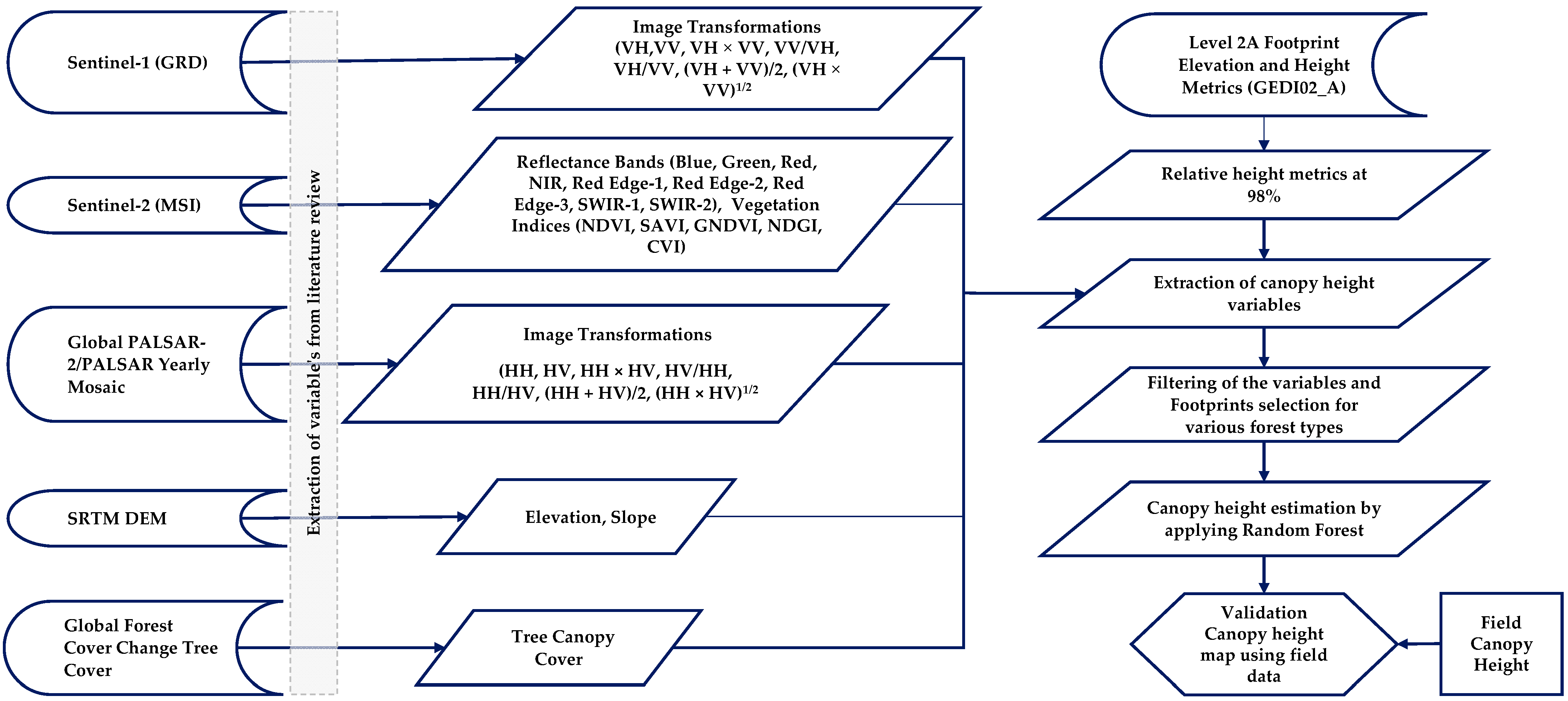
2.1. Multi-Sensor Satellite Data and Pre-Processing

Sentinel-1 is a constellation of two satellites (A and B) flying in near-polar sun-synchronized orbit at an altitude of 697 km. Sentinel-1A and Sentinel-1B can image the whole earth in six days with C-band SAR sensors. It operates with a central frequency of 5.405 GHz and a dual polarization mode (HH + HV, VV + VH). Recently, Sentinel-1B has stopped working due to electronic malfunctions. The pre-processed Sentinel-1 data was accessed from the Google Earth Engine (GEE) platform.
Sentinel-2 is a twin satellite mission orbiting the sun-synchronous orbit phased at 180. It has a high revisit interval of five days at the equator. These provide data continuity to SPOT and LANDSAT missions with broad applications in land management, including forestry, agriculture, water resource, etc. It carries an optical instrument that samples the earth in 13 spectral bands: four bands, six bands, and three bands at spatial resolutions of 10 m, 20 m, and 60 m, respectively. Sentinel-2 Level-1C (S2-L1C) multispectral images were accessed from GEE, providing radiometrically and geometrically corrected, orthorectified top-of-atmosphere (TOA) reflectance data. The spectral bands in the visible, near-infrared, shortwave infrared, and red-edge wavelengths were employed in the current analysis.
PALSAR-2 (Phased Array L-band Synthetic Aperture Radar) on board the ALOS-2 (Advanced Land Observing Satellite), jointly developed by JAXA and the Japan Resources Observation Systems Organization (JAROS), is a SAR sensor that operates at the L-band microwave frequency. It provides continuous data, both day and night, as it is an active sensor. The global 25 m PALSAR/PALSAR-2 mosaic is a seamless global SAR image created by mosaicking strips of individual tiles. The PALSAR/PALSAR-2 images were chosen considering the minimum response to surface moisture. The backscatter values were retrieved using the normalized radar cross section (NRCS) equation. The digital number (DN) values obtained from the calibration process do not show any radar signal from the field structure, illustrated as Sigma nought (σ0) in decibels (dB). The general equation used for the PALSAR-2 image is slightly different from other sensors, due to its normal sine term, already included in the DN values. For Level 1.5 products, the NRCS equation of each polarization component was extracted using Equation (1), with a single calibration factor (CF) of −83 [40].
σ ο = 10 log 10 ( DN 2 ) + CF
where σ0 is the backscattering coefficient in dB, DN is the raw pixel value, and CF is the calibration factor in dB.
The land use land cover (LULC) data from Roy et al. [41] was employed to understand the vegetation type distribution. It exhibits India’s broad vegetation types at 100 m resolution for 1985, 1995, and 2005. A combination of Landsat 4 and 5 Thematic Mapper (TM), Enhanced Thematic Mapper Plus (ETM+), and Multispectral (MSS) data, the Indian Remote Sensing satellites (IRS), the Linear Imaging Self-Scanning Sensor-I and III (LISS-I, LISS-III), and ground surveys were employed for the LULC mapping using the visual interpretation technique. The International Geosphere-Biosphere Programme (IGBP) classification scheme was adopted. The mapping accuracy was assessed, based on 12,606 stratified random sampled ground truth data (Biodiversity Information System, 2014), which indicated more than 90% accuracy [37]. The LULC data is freely available at ORNL DAAC.

2.2. LiDAR GEDI L2A Raster Canopy Top Height (Version 2)

GEDI’s Level 2A Geolocated Elevation and Height Metrics Product (GEDI02_A) comprises 100 relative height (RH) metrics, which collectively describe the waveform collected by GEDI. The original GEDI02_A product is a collection of points with a spatial resolution (footprint) of 25 m. The dataset LARSE/GEDI/GEDI02_A_002_MONTHLY is a raster version of the original GEDI02_A product used in the current study (Table 2).

2.3. Satellite Data-Derived Proxies Used as Predictor Variables

Six spectral bands of Sentinel-2 data were employed (blue, green, red, NIR, RedEdge-1, RedEdge-2, Red Edge-3, SWIR-1, SWIR-2). Five vegetation indices were derived from the surface reflectance data, the normalized difference vegetation index (NDVI), the soil-adjusted vegetation index (SAVI), the green normalized difference vegetation index (GNDVI), the normalized difference greenness index (NDGI), and the chlorophyll vegetation index (CVI). The Sentinel-1 SAR image (VV and VH backscatter bands) and the derived variables as the ratio, average, and square root of the VV and VH were employed as the predictor variables (Table 3). Similarly, the PALSAR-2 SAR image (HH and HV backscatter bands) and the derived variables were used as the ratio, average, and square root of the HH and HV. In addition, the Landsat data derived the tree canopy density, the SRTM DEM elevation and slope were considered as the predictor variables for the tree height estimation (Table 3). All of the determinant variables were resampled at 100 m spatial resolution using the nearest neighbour algorithm to compensate for the variable data resolution and bulk data volume. The canopy height map was produced at 100 m resolution.

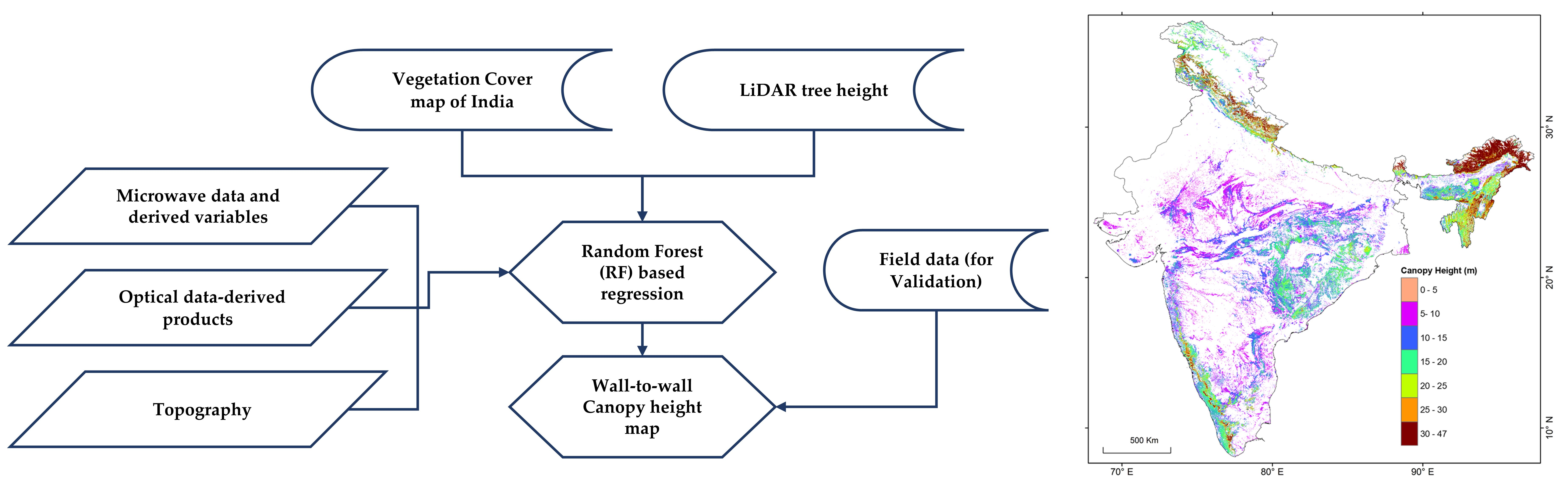
2.4. Canopy Height Prediction Using GEDI and Machine Learning (ML)

Random Forest

The RF regression is an ensemble and supervised learning algorithm combining many decision trees [33]. Previous studies revealed that it has advantages over other ML approaches, such as neural networks and support vector machines, as it provides information on essential variables, is robust, provides a greater accuracy in larger datasets, and has a lower sensitivity in the parameter optimization [42]. The RF algorithm was executed using the random forest library in the R-programming platform with the dependency of the “CARET” package [43]. The RF uses bagging or boosting approaches and the random predictor selection. Usually, 2/3 of the data points of the original dataset are included in a bootstrap sample where 1/3 of the dataset is again excluded from the bootstrap samples, known as out-of-bag (OOB) data [42], which is used to measure the crucial variables. Two hyperparameters were used to improve the model’s accuracy, namely the mtry and ntree values, which were tuned according to the stability and minimum root mean square error (RMSE). The mtry (randomly selected predictors in each node for segregation) is the only hyperparameter for tuning in the CARET package. A grid value ranging from 1 to 10 was passed to the algorithm to autotune the mtry value.
The values of the ancillary variables at the GEDI footprint locations were extracted as a precursor to the model building (Figure S1). The correlation matrix was generated to test the relationship between the LiDAR (GEDI) estimated canopy height and ancillary variables (Figure S2). The dataset (canopy height and corresponding ancillary variable values) was separated into five major vegetation types, based on the India LULC map of 2005. Therefore, the separate models were built for the canopy height prediction for different vegetation types. The vegetation classes included evergreen forest, deciduous forest, mixed forest, plantation, and shrubland. Each dataset for the five vegetation types was further segregated into 70:30 ratios for the model training and validation. The model’s accuracy was assessed, based on the R2, RMSE, and normalized RMSE between the observed and predicted canopy height values for the validation dataset. The overall data processing methodology is shown in Figure 2.

3. Results

3.1. Canopy Height Modelling

The number of GEDI footprints and associated height ranges for the different vegetation types demonstrated a wider data distribution (Table 4). The highest proportion of footprints overlaid on the deciduous forests and the least on the plantation (Figure S1). The canopy height range for different vegetation varies widely, with the highest variation in evergreen forests (1.64 m to 47.23 m) with a mean of 22.75 m. The lowest range was observed for plantations (<1 m to 40 m) with a mean height of 12.75 m. However, the lowest mean canopy height was estimated for shrubland as 7.18 m. The GEDI estimated canopy height has the maximum correlation with TCC as 0.45, 0.59, 0.66, 0.51, and 0.59 for evergreen forests, deciduous forests, mixed forests, plantations, and shrubland (Figure S2). The RF model trained using the GEDI data for various vegetation types indicated an acceptable accuracy, wherein the maximum correlation (R2) was observed for the mixed forest with RMSE 4.94 m and the normalized RMSE of 12.41%. The lowest modelling accuracy was obtained for the plantation (R2: 0.56, RMSE: 5.01 m and the normalized RMSE: 14.32%) (Table 5). A positive bias was observed for the plantation (0.086), wherein the estimated bias was negative for other forest types, such as deciduous forests (−0.03), evergreen forests (−0.029), mixed forests (−0.06) and shrubland (−0.06). Slope and TCC emerged as the best proxy indicators (variable importance of more than 60%) for the canopy height prediction for the evergreen forest and plantation (Figure S3). TCC, Sentinel-1 VH, slope, avg (VV, VH) were crucial predictor variables for the deciduous forest. Slope and Sentinel-1 VV and VH backscatter ratios are essential predictor variables for the mixed forest. In contrast, the slope, elevation, ALOS PLASAR HH and HV backscatter ratio, TCC, Sentinel-1 VV and VH, and vegetation indices, such as SAVI and NDVI, emerged as essential indicators for the shrubland. In summary, the topography, SAR backscatters, tree canopy cover, and vegetation indices (SAVI and NDVI) are the most influential predictors of the canopy height estimation for different vegetation classes.

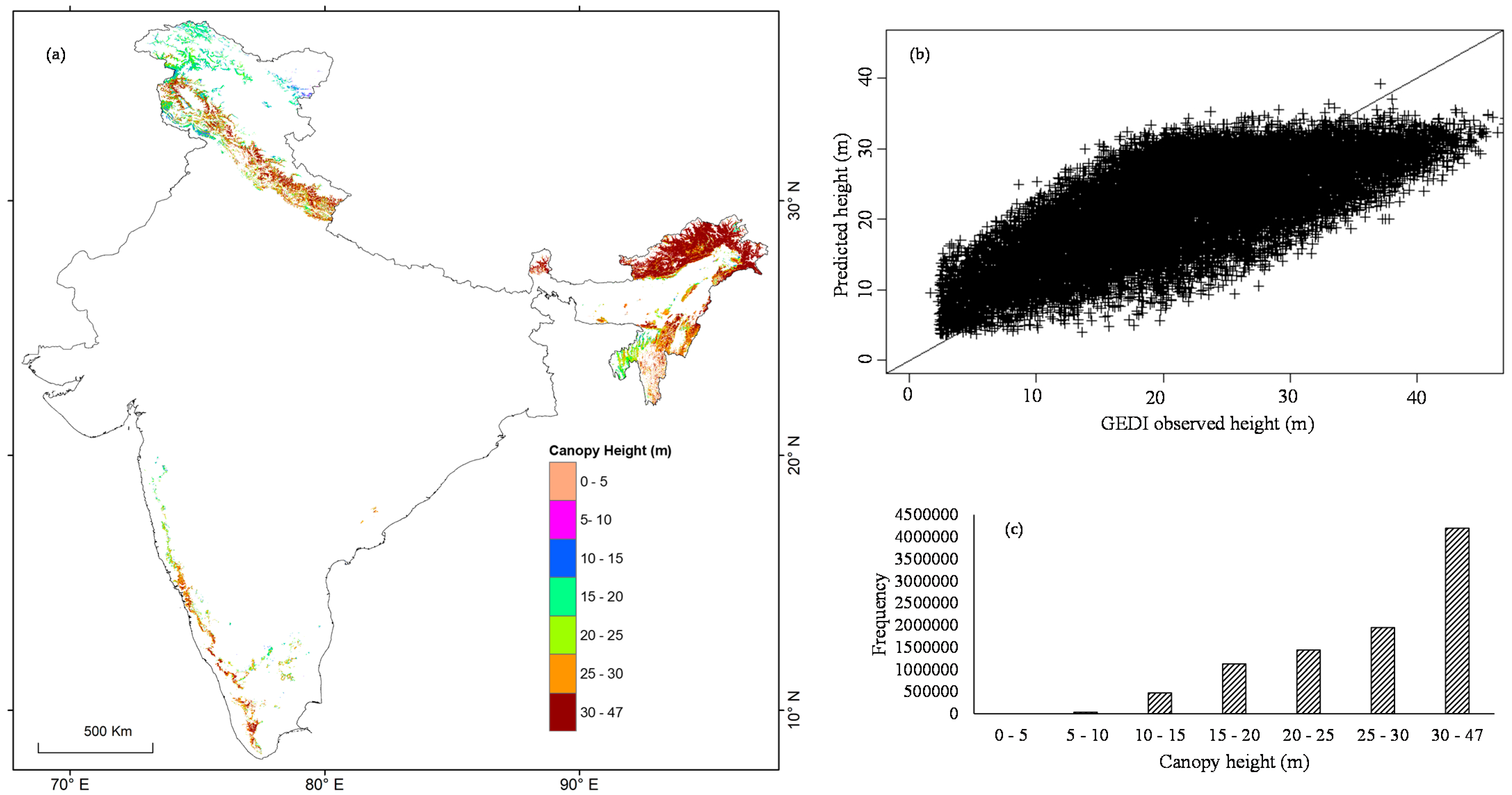
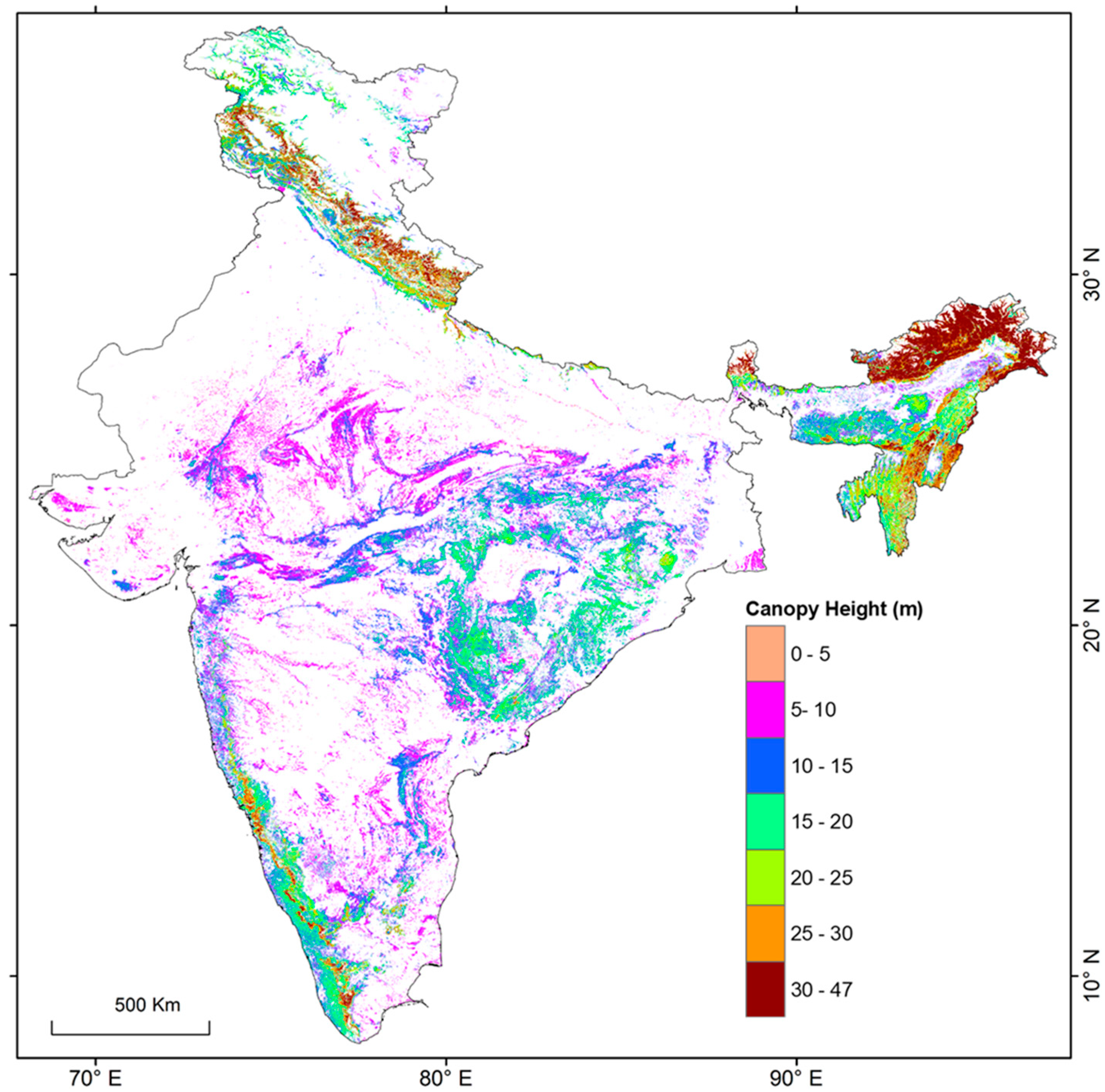
3.2. Canopy Height Mapping

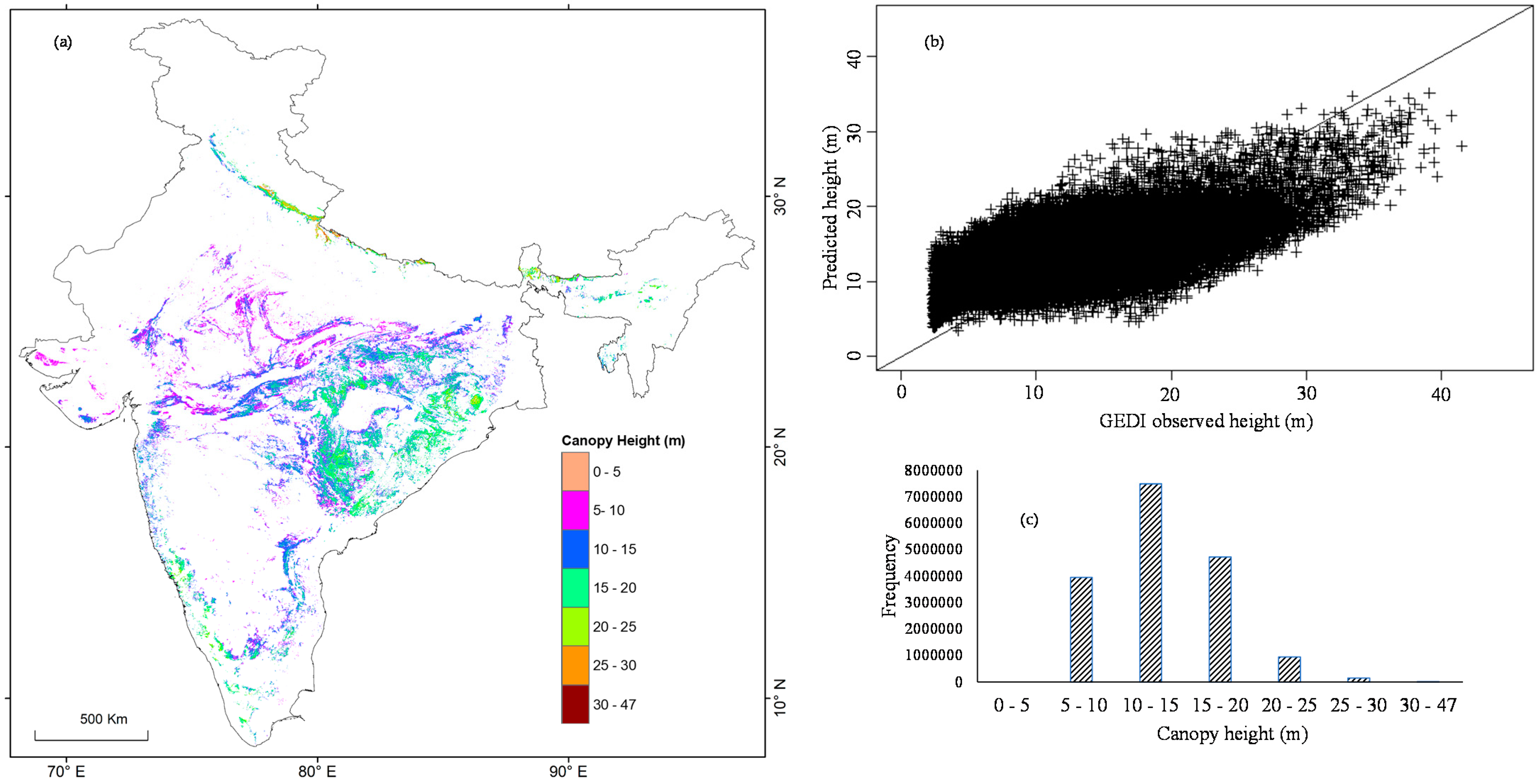
3.2.1. Canopy Height Mapping of the Evergreen Forest

The canopy height maps show a broad range of canopy heights for the evergreen forest. Most evergreen forests are observed in humid and topographically upland regions. The predicted canopy height indicated a good agreement with the observed canopy height (Figure 3b). The estimated canopy height map shows a general trend of a higher canopy height (>30 m) in the rugged terrain of the eastern Himalayan regions, such as Arunachal Pradesh, Sikkim, Manipur, Mizoram, and Nagaland (Figure 3a). A similar higher canopy height is estimated in the Western Ghats and several parts of the Western Himalayan region, such as Uttarakhand, Himachal Pradesh, and Jammu and Kashmir. In contrast, a comparatively lower height (<30 m) is estimated for the rest of the evergreen forest. The distribution of the canopy heights is visualized through the histogram of the images. It shows 45.6% of the total evergreen forest cover with more than a 30 m canopy height, above 94% with more than 15 m (Figure 3c). The estimated mean canopy height for the evergreen forests is 27.93 m (~28 m).

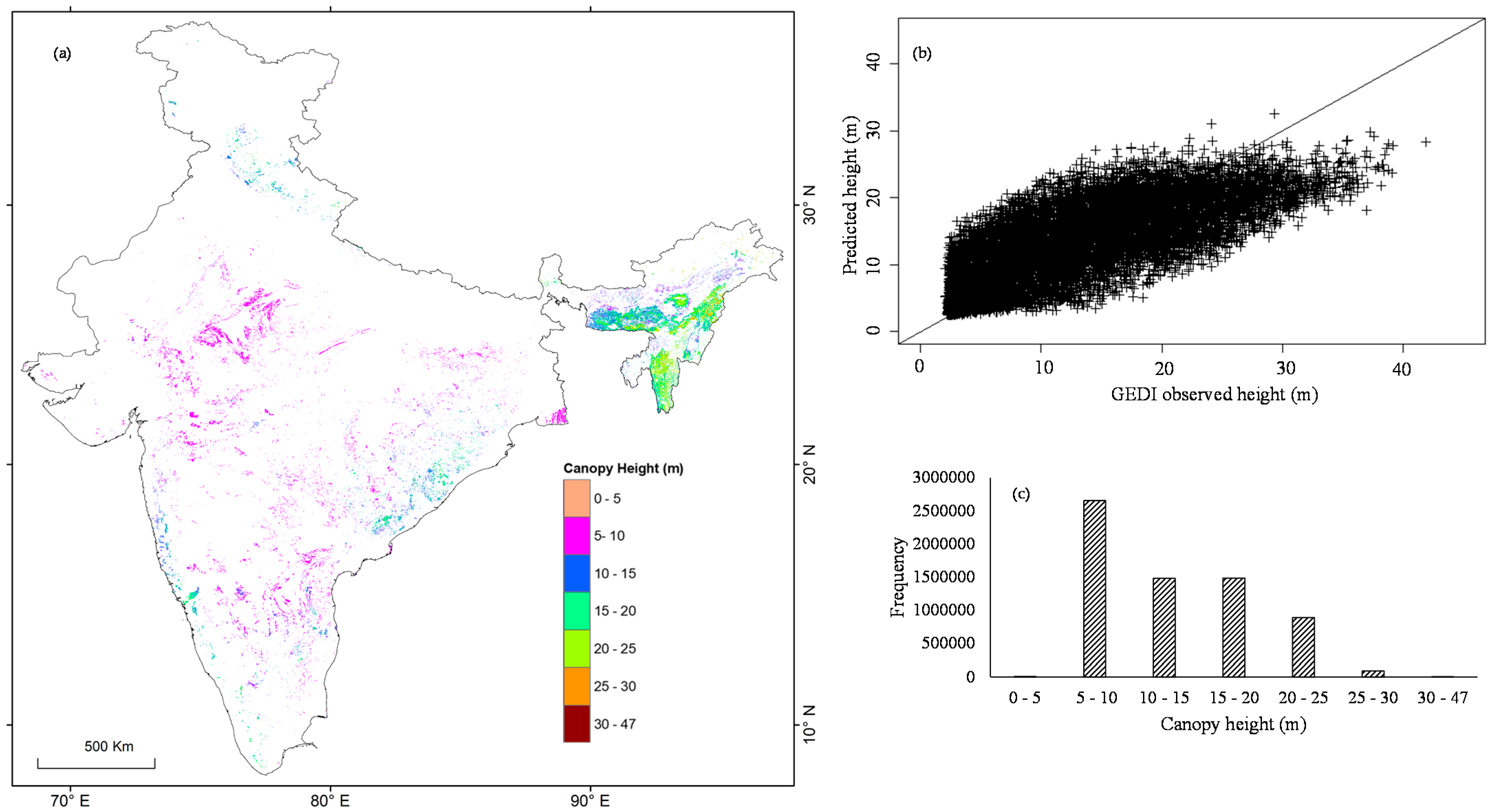
3.2.2. Canopy Height Mapping of the Deciduous Forest

Most of the deciduous forest is observed in the Deccan peninsular regions and foothills of the Himalayan belt. The Deccan peninsular region is characterized by drier regions with a higher population pressure than the evergreen forests (Figure 4a). The estimated canopy height mostly varies from 5 m to 25 m, which encompasses 99% of the total deciduous forest in India (Figure 4b,c). The average estimated canopy height is 13.6 m. Comparatively taller plants (>15 m) are seen in the wet regions, including Odisha, Chhattisgarh, and the Western Ghats. In contrast, the dominant shorter trees (<15 m) are found in drier regions, such as Madhya Pradesh, Gujarat, Rajasthan, Telangana, and Andhra Pradesh.

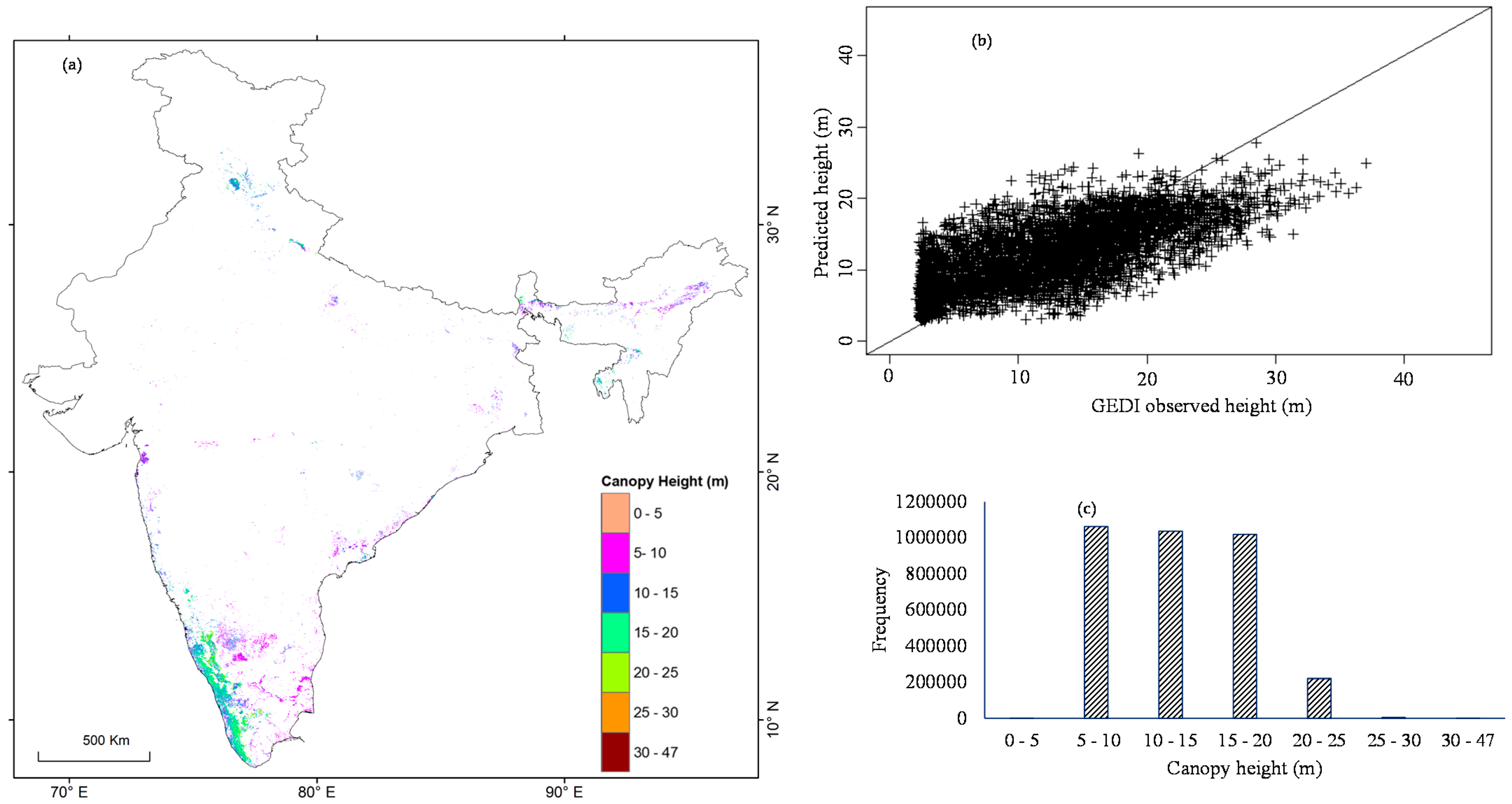
3.2.3. Canopy Height Mapping of the Mixed Forest

The mixed forest is mainly found scattered in the Deccan peninsular region, except in the Northeast Indian states of Meghalaya, Mizoram, Nagaland, and part of Assam. The estimated canopy height map shows taller plants (>15 m) in the wet and humid Northeast India, east coastal and Western Ghats (Figure 4a). In comparison, the shorter plants (<15 m) are seen in the drier Deccan peninsular region. Shorter trees (5–10 m) are seen in 40.2% of the total area, while a 10 m to 25 m canopy height is estimated in 58.3% of the total mixed forest (Figure 5b,c). Above 25 m and below 5 m, the canopy height is seen in only 1.5% of the mixed forest. However, the mean canopy height for the mixed forests is 12.86 m.

3.2.4. Canopy Height Mapping of the Plantation

The plantation is predominantly seen in Southern India, wherein taller trees (>15 m) are found in the wet and rugged terrain of the Western Ghats. On the contrary, shorter trees (<10 m) are found in the drier and topographically flat terrain. A few plantation patches in the Western Himalayan region indicated taller trees, compared to northeast India (Figure 6a). The histogram indicated a nearly equal tree cover distribution (31%) in 5–10 m, 10–15 m, and 15–20 m ranges, encompassing > 93% of the total plantations (Figure 5b,c). The average estimated canopy height is 13.15 m.

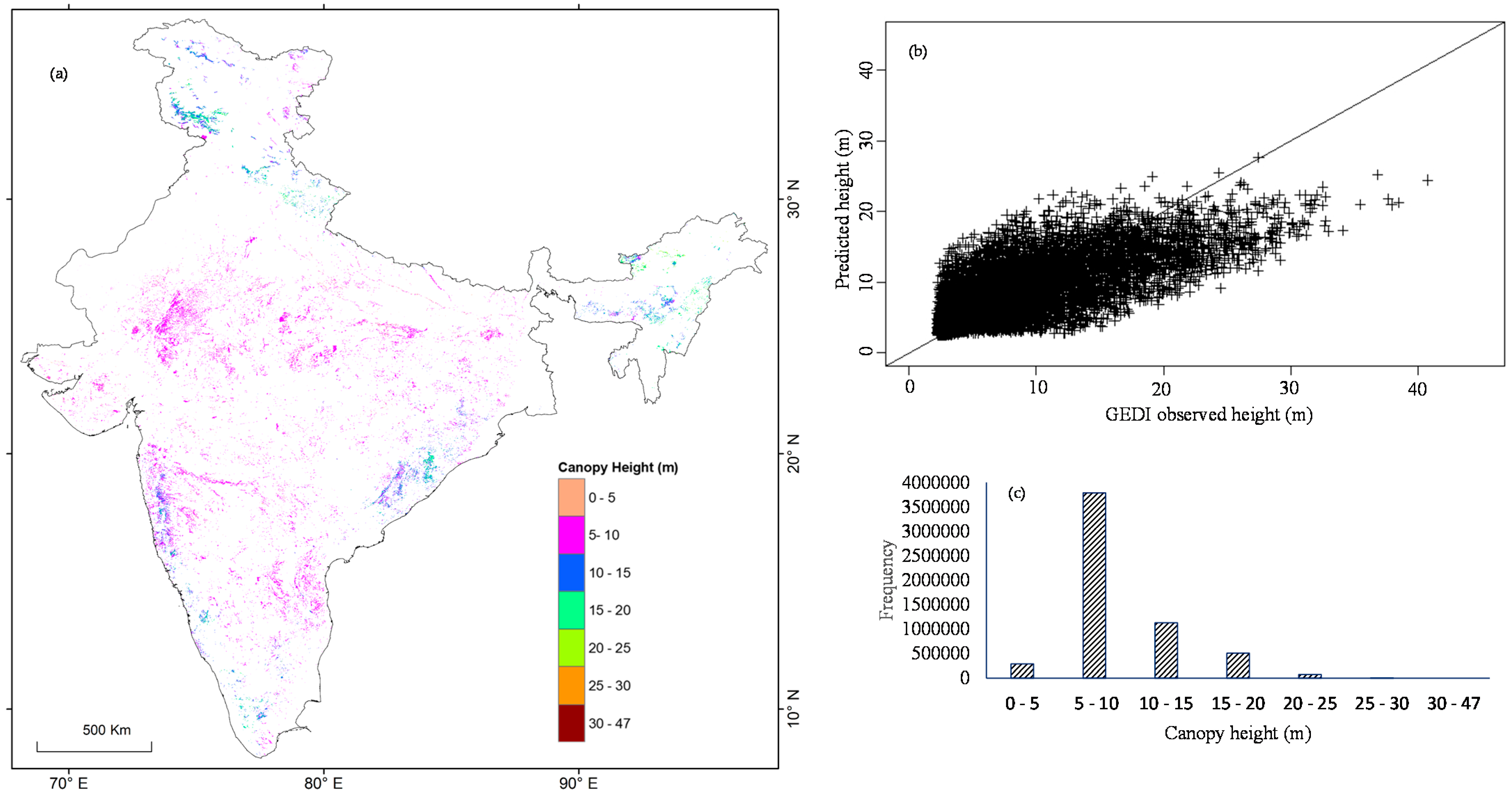
3.2.5. Canopy Height Mapping of the Shrubland

Shrub-dominated areas are also found highly scattered, similar to the mixed forest, which is mostly seen in the Deccan peninsular parts of Northeast India, Western Himalayan and trans-Himalayan regions (Figure 6a). Shorter plant canopies (<10 m) are dominant (>70%), which are seen in the dry and topographically flat terrain of the Deccan peninsular region (Figure 7b,c), while taller canopies (>10 m) are seen in the wet coastal, and rugged terrain of the Northeast, Western Himalayan, and trans-Himalayan regions. The average estimated canopy height is 8.69 m.

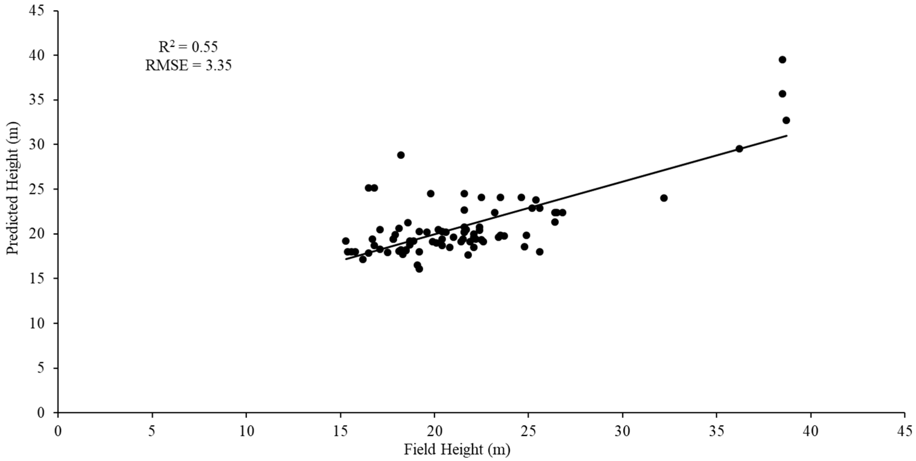
3.3. Canopy Height Map Validation

The estimated canopy height map was validated using the field-collected data from various parts of India (Figure 1). The canopy height data collected in 94 plots using the laser range finder was employed. The ground reference data include 41 plots from the moist deciduous forests of Sikkim, 53 from the moist and dry deciduous forests of the Simlipal National Park, Odisha. The correlation plot between the predicted and field-measured values showed a coefficient of determination of 0.55 and a RMSE of 8.61 (Figure 8).
The estimated canopy height for the different forest types was merged to create a unified forest canopy height map of India (Figure 9). The study suggests that 33.15% of the total forest cover (excluding grassland) has a lower canopy height (<10 m). In comparison, 44.51% have a moderate canopy height (10–20 m), and the rest, 22.34%, have a higher canopy height (>20 m).

4. Discussion

Canopy Height Modelling

The optical and microwave satellite data provide important indicators to model the plant structure. The development of machine-learning models allowed the wall-to-wall tree height mapping at the national scale. Although the canopy height shows a similar height range for the different vegetation classes, there is a significant difference in the mean height. The spatial auto-correlation graphs were generated to highlight the height distribution in relation to distant observations (Figure S4). The highest mean height is observed in the GEDI data for the evergreen forest (22.75 m) and the lowest in shrubland (7.18 m). The GEDI-derived mean canopy height for the deciduous forests, mixed forests and plantations are 12.67 m, 13.22 m, and 12.75 m, respectively. The taller evergreen trees (>30 m) are primarily found in Northeast India’s topography of rugged and wet climate regions, the Western Ghats, Western Himalayan, and trans-Himalayan regions. The shorter evergreen trees (<25 m) are dominantly found in the dry temperate trans-Himalayas and shifting the cultivation-dominated wet and rugged terrain of Tripura and Assam in Northeast India [44]. The distribution of the evergreen forests in different climate zones denotes the water and energy availability, which regulates the tree cover, mortality, and succession. Moreover, the height variations indicate the slope as an important variable in the canopy height prediction for evergreen forests, followed by the canopy density and microwave backscatter values, which segregates the canopy structures. Previous studies also articulated that the slope and canopy cover are essential indicators for the height estimation [29]. Li et al. [45] utilized deep learning and the random forest for the canopy height estimation, based on ICESat-2 LiDAR data by employing Sentinel-1, Sentinel-2, and Landsat data and derived the proxies as predictor variables. They observed a higher accuracy with the Sentinel data than with the Landsat data-based estimates and found the Sentinel-1 backscatter and Sentinel-2 red-edge spectral band as crucial indicators. On the contrary, the deciduous forests are primarily seen in topographically moderate rugged terrain. Moreover, the phenology is an integral characteristic of the deciduous forests, which are well captured by the canopy density and microwave backscatter values. Similar to the evergreen forests, the taller trees (>15 m) are dominantly found in wetter regimes (Himalayan foothills, Western Ghats, and Eastern Ghats) than shorter trees (<15 m) in drier regimes (central India). Similarly, the topography, followed by the microwave backscatter and canopy density, plays an essential role in estimating the canopy height for mixed forests, plantations, and shrublands. Moreover, taller plants are observed in wet regimes and shorter plants in drier regimes, denoting the overall trend of the climate variables that define the tree growth. Global studies have also identified a higher canopy height in wet regimes than in drier regimes, wherein taller trees are reported in the Himalayan region than in other parts of India [29,46].
ML algorithms, such as RF, can establish a complex non-linear relationship between the vegetation information and remote sensing images with indeterminate data distribution and can flexibly combine data from different sources to improve the prediction accuracy [47,48]. The modelling accuracy relies on the spatial resolution of the input predictor variables, their sensitivity to the plant structure (denoted by the correlation), geographic extent, and topography. This study examined 31 predictor variables from multiple sources (Figure S2). We discovered that combining ML algorithms and multi-sensor data, compared to traditional linear models can prevent overfitting and significantly improve the estimation accuracy. The RF-based regression models indicated well-accepted accuracies (R2 varied from 0.5 to 0.64, RMSE from 3.73 m to 6.34 m, and nRMSE from 9.70% to 14.32%). We have observed a minor relative negative bias ranging from −0.06 to 0.086. The accuracies obtained in the current study show a good agreement with past global and regional studies [26,34]. As reported in previous studies, the lower accuracy for plantations could indicate the plant diversity [29]. The field validation data mainly included deciduous forests and a few evergreen forests and showed a well-accepted accuracy of the predicted canopy height map (R2: 0.55 and RMSE: 3.35 m). Many existing studies employed the LiDAR canopy height and multi-sensor data to produce wall-to-wall canopy height maps using ML/DL techniques and reported a similar accuracy, as obtained here. Huang et al. [49] achieved a R2 of 0.92, MAE of 4.31 m, and RMSE of 3.87 m in the tree height estimation for China and the reported slope, red reflectance, and microwave backscatter as important indicators. They have also reported a higher accuracy and a reduced uncertainty (4.58%) due to the addition of the PALSAR data. They observed an average forest height of 16.08 m and reported a minor difference in the mean canopy height for different forest types, supporting the current study outcome. Jiang et al. [50] used a stacking algorithm of MLR, SVM, kNN, and RF to estimate the regional forest canopy height. This study showed that multiple model stacking has significantly reduced the RMSE and achieved the best prediction accuracy (R2 of 0.77 and RMSE of 1.96 m).
The GEDI LiDAR data provides the footprint level (25 m) height estimation. However, the continuous canopy height maps are essential for assessing the forest structure, productivity/carbon stock, ecosystem functionality, forest management activities, deforestation/mortality, monitoring tree growth, etc. Various studies have employed proxy variables to develop regression models for the canopy height prediction [29,51]. The canopy height models built in most of the previous continental scale studies did not use specific models for different vegetation types. Moreover, the topography plays an important role in estimating the canopy height, wherein the taller trees are mostly seen in topographically rugged terrain at higher altitudes, indicating lower anthropogenic disturbances. In addition, the canopy height in Northeast India, excluding Arunachal Pradesh, indicated prominent human disturbances due to shifting cultivation practices in the region [44]. India has six biogeographic zones with significantly diverse environmental conditions determining the dominant vegetation types. Several studies have highlighted the importance of different climatic factors, especially the moisture regulating canopy height [29,31,52]. Similarly, the current study has highlighted the important climate variables that regulate the canopy height distribution. The current study generated the canopy height map at 100 m spatial resolution, which thus didn’t use coarse resolution climate data. It is also apparent that the influencing variables differ, depending on the vegetation type and spatial distribution. The current study clearly shows the canopy density and backscatter values, which indicates the plant structure and growth as important variables for the height estimation. The present study suggests building different models for different vegetation types working at the continental scale.

5. Conclusions

The annual canopy height estimation is essential for understanding the alteration in the ecosystem structure and its functioning, tree growth, generation and recruitment, disturbances, management activities, etc. It is an integral part of the plant biomass and carbon stock estimation. An accurate canopy height map will reduce uncertainty in the estimated carbon storage in Indian tropical forests. The availability of the GEDI LiDAR footprint data in the public domain has opened new possibilities for generating wall-wall tree height maps for large geographic areas. The current study shows that spaceborne LiDAR tree height data with various proxy parameters, such as the satellite data-derived vegetation indices, the microwave backscatter and topography, can be employed for the tree height prediction at a continental scale. Slope, tree canopy density, and backscatter values emerged as the most important proxy indicators. Several models are available for estimating the canopy height, each of which has benefits and disadvantages. In this study, predicting the canopy height using the GEDI data provides a clear understanding of how canopy height relates to its covariates. Further studies could use this information to improve and build a more accurate model. The seamless national scale canopy height map may be utilized in ecological studies, ongoing tree-based restoration monitoring, carbon stock assessment and marketing to national policy formations.

Supplementary Materials

The following are available online at https://www.mdpi.com/article/10.3390/rs14235968/s1. Figure S1. GEDI Footprints for (a) Evergreen Forest, (b) Deciduous Forest, (c) Mixed Forest, (d) Plantation and (e) Shrubland. Figure S2. Correlation Plot between predictor variables and Canopy Height for (a) Evergreen Forests, (b) Deciduous Forests, (c) Mixed Forests, (d) Plantations, (e) Shrubland. Figure S3. Variable importance chart for (a) Evergreen Forest, (b) Deciduous Forest, (c) Mixed Forest, (d) Plantation and (e) Shrubland. Figure S4. Spatial Auto Correlation for (a) Evergreen Forest, (b) Deciduous Forest, (c) Mixed Forest, (d) Plantation and (e) Shrubland.

Author Contributions

Conceptualization, S.M.G. and M.D.B.; methodology, S.M.G., M.D.B., A.J.P. and P.D.; software, S.M.G. and S.K.; validation, S.M.G., S.K. and M.D.B.; formal analysis, S.M.G. and S.K.; investigation, S.M.G., S.K. and M.D.B.; resources, M.D.B. and P.K.B.; data curation, S.M.G. and S.K.; writing—original draft preparation, S.M.G., S.K., A.J.P., P.D. and M.D.B.; writing—supervision, M.D.B., P.S.R., S.K.B. (Saroj K. Barikand), P.K.B., C.J., S.K.B. (Soumit K. Behera) and P.K.S.; visualization, S.M.G., S.K., A.J.P. and M.D.B.; project administration, M.D.B. and P.K.B.; funding acquisition, P.K.B. and M.D.B. All authors have read and agreed to the published version of the manuscript.

Funding

This research was funded by Department of Science & Technology—Centre of Excellence in Climate Change (DST CoE), Government of India [DST/CCP/CoE/79/2017(G), Dt. 30-03-2017], and The APC is funded by a few authors.

Data Availability Statement

The data presented in this study are available on request from the corresponding author.

Acknowledgments

MDB thanks the authorities of the Centre for Oceans, Rivers, Atmosphere and Land Sciences (CORAL), and the Indian Institute of Technology Kharagpur, for supporting the investigation. S.M.G., M.D.B., and P.K.B. thank the Department of Science and Technology (DST), New Delhi, for providing financial support under the ‘Centre of Excellence on Climate Change’ to carry out the study.

Conflicts of Interest

The authors declare no conflict of interest. The funders had no role in the design of the study; in the collection, analyses, or interpretation of the data; in the writing of the manuscript, or in the decision to publish the results.

References

  1. Roy, S.; Mudi, S.; Das, P.; Ghosh, S.; Shit, P.K.; Bhunia, G.S.; Kim, J. Estimating Above Ground Biomass (AGB) and Tree Density Using Sentinel-1 Data. In Spatial Modeling in Forest Resources Management; Springer: Berlin/Heidelberg, Germany, 2021; pp. 259–280. [Google Scholar]
  2. Mensah, S.; Egeru, A.; Assogbadjo, A.E.; Kakaï, R.G. Vegetation structure, dominance patterns and height growth in an Afromontane forest, Southern Africa. J. For. Res. 2020, 31, 453–462. [Google Scholar] [CrossRef]
  3. Fahey, T.J.; Sherman, R.E.; Tanner, E.V. Tropical montane cloud forest: Environmental drivers of vegetation structure and ecosystem function. Trop. Ecol. 2016, 32, 355–367. [Google Scholar] [CrossRef] [Green Version]
  4. Feldpausch, T.R.; Banin, L.; Phillips, O.L.; Baker, T.R.; Lewis, S.L.; Quesada, C.A.; Affum-Baffoe, K.; Arets, E.J.M.M.; Berry, N.J.; Bird, M.; et al. Height-diameter allometry of tropical forest trees. Biogeosciences 2011, 8, 1081–1106. [Google Scholar] [CrossRef] [Green Version]
  5. Ruiz, J.; Fandiño, M.C.; Chazdon, R.L. Vegetation Structure, Composition, and Species Richness across a 56-year Chronosequence of Dry Tropical Forest on Providencia Island, Colombia. Biotrop. Biol. Conserv. 2005, 37, 520–530. [Google Scholar]
  6. Solberg, S.; Hansen, E.H.; Gobakken, T.; Naessset, E.; Zahabu, E. Biomass and InSAR height relationship in a dense tropical forest. Remote Sens. Environ. 2017, 192, 166–175. [Google Scholar] [CrossRef]
  7. Babcock, C.; Finley, A.O.; Bradford, J.B.; Kolka, R.; Birdsey, R.; Ryan, M.G. LiDAR based prediction of forest biomass using hierarchical models with spatially varying coefficients. Remote Sens. Environ. 2015, 169, 113–127. [Google Scholar] [CrossRef] [Green Version]
  8. Laurin, G.V.; Chen, Q.; Lindsell, J.A.; Coomes, D.A.; Del Frate, F.; Guerriero, L.; Pirotti, F.; Valentini, R. Above ground biomass estimation in an African tropical forest with LiDAR and hyperspectral data. ISPRS J. Photogramm. Remote Sens. 2014, 89, 49–58. [Google Scholar] [CrossRef]
  9. Takagi, K.; Yone, Y.; Takahashi, H.; Sakai, R.; Hojyo, H.; Kamiura, T.; Nomura, M.; Liang, N.; Fukazawa, T.; Miya, H.; et al. Forest biomass and volume estimation using airborne LiDAR in a cool-temperate forest of northern Hokkaido, Japan. Ecol. Inform. 2015, 26, 54–60. [Google Scholar] [CrossRef]
  10. Rosen, P.A.; Hensley, S.; Joughin, I.R.; Li, F.K.; Madsen, S.N.; Rodriguez, E.; Goldstein, R.M. Synthetic aperture radar interferometry. Proc. IEEE 2000, 88, 333–382. [Google Scholar] [CrossRef]
  11. Behera, M.D.; Roy, P.S. Lidar Remote Sensing for Forestry Applications: The Indian Context. Curr. Sci. 2002, 83, 1320–1328. [Google Scholar]
  12. Zwally, H.J.; Schutz, B.; Abdalati, W.; Abshire, J.; Bentley, C.; Brenner, A.; Bufton, J.; Dezio, J.; Hancock, D.; Harding, D.; et al. ICESat’s laser measurements of polar ice, atmosphere, ocean, and land. J. Geodyn. 2002, 34, 405–445. [Google Scholar] [CrossRef] [Green Version]
  13. Baccini, A.; Laporte, N.; Goetz, S.J.; Sun, M.; Dong, H. A first map of tropical Africa’s aboveground biomass derived from satellite imagery. Environ. Res. Lett. 2008, 3, 045011. [Google Scholar] [CrossRef]
  14. Baccini, A.G.S.J.; Goetz, S.J.; Walker, W.S.; Laporte, N.T.; Sun, M.; Sulla-Menashe, D.; Hackler, J.L.; Beck, P.S.A.; Dubayah, R.O.; Friedl, M.A.; et al. Estimated carbon dioxide emissions from tropical deforestation improved by carbon-density maps. Nat. Clim. Chang. 2012, 2, 182–185. [Google Scholar] [CrossRef]
  15. Saatchi, S.S.; Harris, N.L.; Brown, S.; Lefsky, M.; Mitchard, E.T.; Salas, W.; Zutta, B.R.; Buermann, W.; Lewis, S.L.; Hagen, S.; et al. Benchmark map of forest carbon stocks in tropical regions across three continents. Proc. Natl. Acad. Sci. USA 2011, 108, 9899–9904. [Google Scholar] [CrossRef] [Green Version]
  16. Markus, T.; Neumann, T.; Martino, A.; Abdalati, W.; Brunt, K.; Csatho, B.; Farrell, S.; Fricker, H.; Gardner, A.; Harding, D.; et al. The Ice, Cloud, and land Elevation Satellite-2 (ICESat-2): Science requirements, concept, and implementation. Remote Sens. Environ. 2017, 190, 260–273. [Google Scholar] [CrossRef]
  17. Neuenschwander, A.; Pitts, K. Ice, Cloud, and Land Elevation Satellite 2 (ICESat-2) Algorithm Theoretical Basis Document (ATBD) for Land-Vegetation along-Track Products (ATL08). Applied Research Laboratory, University of Texas, Austin, TX. 2019. Available online: https://icesat-2.gsfc.nasa.gov/sites/default/files/page_files/ICESat2_ATL08_ATBD_r002_v2.pdf (accessed on 29 September 2022).
  18. Narine, L.L.; Popescu, S.; Neuenschwander, A.; Zhou, T.; Srinivasan, S.; Harbeck, K. Estimating aboveground biomass and forest canopy cover with simulated ICESat-2 data. Remote Sens. Environ. 2019, 224, 1–11. [Google Scholar] [CrossRef]
  19. Neuenschwander, A.L.; Magruder, L.A. Canopy and Terrain Height Retrievals with ICESat-2: A First Look. Remote Sens. 2019, 11, 1721. [Google Scholar] [CrossRef] [Green Version]
  20. Guerra-Hernández, J.; Narine, L.L.; Pascual, A.; Gonzalez-Ferreiro, E.; Botequim, B.; Malambo, L.; Neuenschwander, A.; Popescu, S.C.; Godinho, S. Aboveground Biomass Mapping by Integrating ICESat-2, SENTINEL-1, SENTINEL-2, ALOS2/PALSAR2, and Topographic Information in Mediterranean Forests. GISci. Remote Sens. 2022, 59, 1509–1533. [Google Scholar] [CrossRef]
  21. Dubayah, R.; Blair, J.B.; Goetz, S.; Fatoyinbo, L.; Hansen, M.; Healey, S.; Hofton, M.; Hurtt, G.; Kellner, J.; Luthcke, S.; et al. The Global Ecosystem Dynamics Investigation: High-resolution laser ranging of the earth’s forests and topography. Sci. Remote sens. 2020, 1, 100002. [Google Scholar] [CrossRef]
  22. Joshi, N.; Mitchard, E.T.A.; Brolly, M.; Schumacher, J.; Fernández-Landa, A.; Johannsen, V.K.; Marchamalo, M.; Fensholt, R. Understanding “saturation” of Radar Signals over Forests. Sci. Rep. 2017, 7, 3505. [Google Scholar] [CrossRef] [PubMed] [Green Version]
  23. Behera, M.D.; Tripathi, P.; Mishra, B.; Kumar, S.; Chitale, V.S.; Behera, S.K. Above-Ground Biomass and Carbon Estimates of Shorea Robusta and Tectona Grandis Forests Using QuadPOL ALOS PALSAR Data. Adv. Space Res. 2016, 57, 552–561. [Google Scholar] [CrossRef]
  24. Sothe, C.; Gonsamo, A.; Lourenço, R.B.; Kurz, W.A.; Snider, J. Spatially Continuous Mapping of Forest Canopy Height in Canada by Combining GEDI and ICESat-2 with PALSAR and Sentinel. Remote Sens. 2022, 14, 5158. [Google Scholar] [CrossRef]
  25. Lang, N.; Kalischek, N.; Armston, J.; Schindler, K.; Dubayah, R.; Wegner, J.D. Global Canopy Height Regression and Uncertainty Estimation from GEDI LIDAR Waveforms with Deep Ensembles. Remote Sens. Environ. 2022, 268, 112760. [Google Scholar] [CrossRef]
  26. Liu, X.; Su, Y.; Hu, T.; Yang, Q.; Liu, B.; Deng, Y.; Tang, H.; Tang, Z.; Fang, J.; Guo, Q. Neural Network Guided Interpolation for Mapping Canopy Height of China’s Forests by Integrating GEDI and ICESat-2 Data. Remote Sens. Environ. 2022, 269, 112844. [Google Scholar] [CrossRef]
  27. Adam, M.; Urbazaev, M.; Dubois, C.; Schmullius, C. Accuracy Assessment of GEDI Terrain Elevation and Canopy Height Estimates in European Temperate Forests: Influence of Environmental and Acquisition Parameters. Remote Sens. 2020, 12, 3948. [Google Scholar] [CrossRef]
  28. Fayad, I.; Ienco, D.; Baghdadi, N.; Gaetano, R.; Alvares, C.A.; Stape, J.L.; Ferraço Scolforo, H.; Le Maire, G. A CNN-Based Approach for the Estimation of Canopy Heights and Wood Volume from GEDI Waveforms. Remote Sens. Environ. 2021, 265, 112652. [Google Scholar] [CrossRef]
  29. Potapov, P.; Li, X.; Hernandez-Serna, A.; Tyukavina, A.; Hansen, M.C.; Kommareddy, A.; Pickens, A.; Turubanova, S.; Tang, H.; Silva, C.E.; et al. Mapping Global Forest Canopy Height through Integration of GEDI and Landsat Data. Remote Sens. Environ. 2021, 253, 112165. [Google Scholar] [CrossRef]
  30. Dorado-Roda, I.; Pascual, A.; Godinho, S.; Silva, C.A.; Botequim, B.; Rodríguez-Gonzálvez, P.; González-Ferreiro, E.; Guerra-Hernández, J. Assessing the Accuracy of GEDI Data for Canopy Height and Aboveground Biomass Estimates in Mediterranean Forests. Remote Sens. 2021, 13, 2279. [Google Scholar] [CrossRef]
  31. Simard, M.; Pinto, N.; Fisher, J.B.; Baccini, A. Mapping forest canopy height globally with spaceborne LiDAR. J. Geophys. Res. Biogeosci. 2011, 116, 1–12. [Google Scholar] [CrossRef] [Green Version]
  32. Wang, Y.; Li, G.; Ding, J.; Guo, Z.; Tang, S.; Wang, C.; Huang, Q.; Liu, R.; Chen, J.M. A combined GLAS and MODIS estimation of the global distribution of mean forest canopy height. Remote Sens. Environ. 2016, 174, 24–43. [Google Scholar] [CrossRef]
  33. Breiman, L. Random Forests. Mach. Learn. 2001, 45, 5–32. [Google Scholar] [CrossRef] [Green Version]
  34. Tripathi, P.; Behera, M.D. Plant Height Profiling in Western India Using LiDAR Data. Curr. Sci. 2013, 105, 970–977. [Google Scholar]
  35. Ghosh, S.M.; Behera, M.D. Forest Canopy Height Estimation Using Satellite Laser Altimetry: A Case Study in the Western Ghats, India. Appl. Geomat. 2017, 9, 159–166. [Google Scholar] [CrossRef]
  36. Schlund, M.; Wenzel, A.; Camarretta, N.; Stiegler, C.; Erasmi, S. Vegetation Canopy Height Estimation in Dynamic Tropical Landscapes with TanDEM-X Supported by GEDI Data. Methods Ecol. Evol. 2022, 1–18. [Google Scholar] [CrossRef]
  37. Lin, X.; Xu, M.; Cao, C.; Dang, Y.; Bashir, B.; Xie, B.; Huang, Z. Estimates of Forest Canopy Height Using a Combination of ICESat-2/ATLAS Data and Stereo-Photogrammetry. Remote Sens. 2020, 12, 3649. [Google Scholar] [CrossRef]
  38. Gupta, R.; Sharma, L.K. Mixed Tropical Forests Canopy Height Mapping from Spaceborne LiDAR GEDI and Multisensor Imagery Using Machine Learning Models. Remote Sens. Appl. Soc. Environ. 2022, 27, 100817. [Google Scholar] [CrossRef]
  39. Rishmawi, K.; Huang, C.; Zhan, X. Monitoring Key Forest Structure Attributes across the Conterminous United States by Integrating GEDI LiDAR Measurements and VIIRS Data. Remote Sens. 2021, 13, 442. [Google Scholar] [CrossRef]
  40. Shimada, M.; Isoguchi, O.; Tadono, T.; Isono, K. PALSAR Radiometric and Geometric Calibration. IEEE Trans. Geosci. Remote Sens. 2009, 47, 3915–3932. [Google Scholar] [CrossRef]
  41. Roy, P.S.; Roy, A.; Joshi, P.K.; Kale, M.P.; Srivastava, V.K.; Srivastava, S.K.; Dwevidi, R.S.; Joshi, C.; Behera, M.D.; Meiyappan, P. Development of Decadal (1985–1995–2005) Land Use and Land Cover Database for India. Remote Sens. 2015, 7, 2401–2430. [Google Scholar] [CrossRef] [Green Version]
  42. Cutler, D.R.; Edwards Jr, T.C.; Beard, K.H.; Cutler, A.; Hess, K.T.; Gibson, J.; Lawler, J.J. Random Forests for Classification in Ecology. Ecology 2007, 88, 2783–2792. [Google Scholar] [CrossRef]
  43. Kuhn, M. Building Predictive Models in R Using the caret Package. J. Stat. Softw. 2008, 28, 1–26. [Google Scholar] [CrossRef] [Green Version]
  44. Das, P.; Mudi, S.; Behera, M.D.; Barik, S.K.; Mishra, D.R.; Roy, P.S. Automated Mapping for Long-Term Analysis of Shifting Cultivation in Northeast India. Remote Sens. 2021, 13, 1066. [Google Scholar] [CrossRef]
  45. Li, W.; Niu, Z.; Shang, R.; Qin, Y.; Wang, L.; Chen, H. High-Resolution Mapping of Forest Canopy Height Using Machine Learning by Coupling ICESat-2 LiDAR with Sentinel-1, Sentinel-2 and Landsat-8 Data. Int. J. Appl. Earth Obs. Geoinf. 2020, 92, 102163. [Google Scholar] [CrossRef]
  46. Lang, N.; Jetz, W.; Schindler, K.; Wegner, J.D. A High-Resolution Canopy Height Model of the Earth. arXiv 2022, arXiv:2204.08322. [Google Scholar]
  47. Ghosh, S.M.; Behera, M.D.; Paramanik, S. Canopy Height Estimation Using Sentinel Series Images through Machine Learning Models in a Mangrove Forest. Remote Sens. 2020, 12, 1519. [Google Scholar] [CrossRef]
  48. Prakash, A.J.; Behera, M.D.; Ghosh, S.M.; Das, A.; Mishra, D.R. A New Synergistic Approach for Sentinel-1 and PALSAR-2 in a Machine Learning Framework to Predict Aboveground Biomass of a Dense Mangrove Forest. Ecol. Inform. 2022, 72, 101900. [Google Scholar] [CrossRef]
  49. Huang, H.; Liu, C.; Wang, X. Constructing a Finer-Resolution Forest Height in China Using ICESat/GLAS, Landsat and ALOS PALSAR Data and Height Patterns of Natural Forests and Plantations. Remote Sens. 2019, 11, 1740. [Google Scholar] [CrossRef] [Green Version]
  50. Jiang, F.; Zhao, F.; Ma, K.; Li, D.; Sun, H. Mapping the Forest Canopy Height in Northern China by Synergizing ICESat-2 with Sentinel-2 Using a Stacking Algorithm. Remote Sens. 2021, 13, 1535. [Google Scholar] [CrossRef]
  51. Ghosh, S.M.; Behera, M.D.; Jagadish, B.; Das, A.K.; Mishra, D.R. A Novel Approach for Estimation of Aboveground Biomass of a Carbon-Rich Mangrove Site in India. J. Environ. Manag. 2021, 292, 112816. [Google Scholar] [CrossRef]
  52. Dubayah, R.; Luthcke, S.; Sabaka, T.; Nicholas, J.; Preaux, S.; Hofton, M. GEDI L3 Gridded Land Surface Metrics, Version 1; ORNL DAAC: Oak Ridge, TN, USA, 2021. [Google Scholar] [CrossRef]
Figure 1. Study area. India land cover map (representing only the major forest covers).
Remotesensing 14 05968 g001
Figure 2. Methodological flow diagram for predicting the canopy height using the GEDI canopy height data by applying the decision tree-based machine learning (ML) algorithm.
Remotesensing 14 05968 g002
Figure 3. (a) GEDI predicted forest canopy height map, (b) the RF model predicted vs. the field-estimated height plot using the GEDI data and (c) histograms showing the canopy height distribution for the evergreen forests.
Remotesensing 14 05968 g003
Figure 4. (a) GEDI predicted forest canopy height map, (b) the RF model predicted vs. the field-estimated height plot using GEDI data and (c) histograms showing the canopy height distribution for the deciduous forests.
Remotesensing 14 05968 g004
Figure 5. (a) GEDI predicted forest canopy height map, (b) the RF model predicted vs. the field-estimated height plot using the GEDI data and (c) histograms showing the canopy height distribution for the mixed forest.
Remotesensing 14 05968 g005
Figure 6. (a) GEDI predicted forest canopy height map, (b) the RF model predicted vs. the field-estimated height plot using the GEDI data and (c) histograms showing the canopy height distribution for plantations.
Remotesensing 14 05968 g006
Figure 7. (a) GEDI predicted forest canopy height map, (b) the RF model predicted vs. the field-estimated height plot using the GEDI data and (c) histograms showing the canopy height distribution for the shrubland.
Remotesensing 14 05968 g007
Figure 8. Validation of the canopy height map, based on the field observations.
Remotesensing 14 05968 g008
Figure 9. Unified canopy height map of India’s forest cover (excluding grassland).
Remotesensing 14 05968 g009
Table 1. Past studies on the canopy height estimation studies using the GEDI LiDAR data.
S. NoStudyMethodR2RMSE (m)MAE (m)Bias (m)Reference
1GlobalConvolutional Neural Network (CNN) Model-3.602.1−1.0 to −0.1[25]
2RegionalNeural Network Guided Interpolation (NNGI)0.584.93-−1.42[26]
3RegionalComparison of GEDI-CHM and ALS-CHM0.27–0.34---[27]
4RegionalConvolutional Neural Network (CNN) Model0.86–0.911.54–1.94--[28]
5GlobalMachine-Learning Algorithm (regression tree)0.626.604.45-[29]
6RegionalNon-Linear Regression0.49–0.711.95–3.96-Dehesas (−0.50), Encinares (0.39), Alcornocales (−0.06), Pinaster (−0.97), and Pinea (0.27)[30]
7RegionalSemi-Empirical Models0.42–0.626.89–10.25-0.7–−0.8[36]
8RegionalArtificial Neural Network (ANN) Model0.513.34–3.47--[37]
9RegionalBayesian Regularization for Feed-Forward Neural Networks (BRNNs)0.494.683.66-[38]
10RegionalRandom Forest Regression0.803.352.09-[39]
Table 2. List of data used in the study.
S. NoDataDateSourceSpatial Resolution (m)Product Details
1GEDI Level 2A Height Metric2021GEE25Relative Height Metrics at 98% (rh98)
2Sentinel-1 (GRD)2021GEE10(Polarization: VH, VV)
3Sentinel-2 MSI2021GEE30(Bands: Blue, Green, Red, Re, NIR, Edge 1, RedEdge 2, RedEdge 3, SWIR 1, SWIR 2)
4SRTM DEM-GEE30(Slope, Elevation)
5Global PALSAR-2/PALSAR Yearly Mosaic2021GEE25(Polarization: HH, HV)
6Landsat data derived Vegetation Continuous Fields (VCF) tree cover2015GEE30Tree Canopy Cover (%)
Table 3. Predictor variables used to run the model.
S. NoDataPredictor Variables
1Sentinel-1VV, VH, VH∗VV, VH/VV, VV/VH, Average (VH, VV), Square root (VH, VV)
2PALSAR-2/PALSARHH, HV, HH∗HV, HH/HV, HV/HH, Average (HH, HV), Square root (HH, HV)
3Sentinel-2Blue, Green, Red, NIR, Red Edge-1, Red Edge-2, Red Edge-3, SWIR-1, SWIR-2,
4Sentinel-2 Vegetation IndicesNormalized Difference Vegetation Index (NDVI), Soil Adjusted Vegetation Index (SAVI), Green Normalized Difference Vegetation Index (GNDVI), Normalized Difference Green Index (NDGI), Chlorophyll Vegetation Index (CVI)
5SRTM DEMElevation, Slope
6Landsat Vegetation Tree CoverTree Canopy Cover
Table 4. GEDI footprints and canopy height range for the different vegetation classes.
Forest TypeObservation FootprintsMax (m)Min (m)Mean (m)
Evergreen Forest62,09747.231.6422.75
Deciduous Forest106,33542.471.6812.67
Mixed Forest40,08442.291.8713.22
Plantation16,34039.890.0312.75
Shrubland33,00740.711.757.18
Table 5. Error analysis and model validation for the different forest types (p-values < 0.001).
S. NoForest TypeR2RMSE (m)nRMSE (%)Relative Bias
1Evergreen Forest0.556.3413.60−0.029
2Deciduous Forest0.566.0112.54−0.03
3Mixed Forest0.644.9412.41−0.06
4Plantation0.505.0114.320.086
5Shrubland0.603.739.70−0.06
Publisher’s Note: MDPI stays neutral with regard to jurisdictional claims in published maps and institutional affiliations.

