Coastline Recognition Algorithm Based on Multi-Feature Network Fusion of Multi-Spectral Remote Sensing Images

Abstract

Remote sensing images can obtain broad geomorphic features and provide a strong basis for analysis and decision making. As 71% of the earth is covered by water, shipping has become an efficient means of international trade and transportation, and the development level of coastal cities will directly reflect the development level of a country. The coastline is the boundary line between seawater and land, so it is of great significance to accurately identify it to assist shipping traffic and docking, and this identification will also play a certain auxiliary role in environmental analysis. Currently, the main problems of coastline recognition conducted by remote sensing images include: (1) in the process of remote sensing, image transmission inevitably brings noise causing poor image quality and difficult image quality enhancement; (2) s single scale does not allow for the identification of coastlines at different scales; and (3) features are under-utilized, false detection is high and intuitive measurement is difficult. To address these issues, we used the following multispectral methods: (1) a PCA-based image enhancement algorithm was proposed to improve image quality; (2) a dual attention network and HRnet network were proposed to extract suspected coastlines from different levels; and (3) a decision set fusion approach was proposed to transform the coastline identification problem into a probabilistic problem for coastline extraction. Finally, we constructed a coastline straightening model to visualize and analyze the recognition effect. Experiments showed that the algorithm has an AOM greater than 0.88 and can achieve coastline extraction.

1. Introduction

The sea and the land are the geomorphological units on the surface of the earth, and the boundary line between seawater and land becomes the coastal zone [1]. The location of the coastline is an important part of determining the remote sensing survey of an island’s coastal zone. Coastline information is the basis for measuring and calibrating terrestrial and water resources and is the foundation for the excavation and management of coastal zone resources. The location and orientation of the coastline provides the most basic information for automated ship navigation, coastline erosion monitoring, and modelling, etc. The analysis of coastline lengths and changing coast sections is a prerequisite for carrying out the evolution of the natural environment [2]. Therefore, rapid and accurate coastline extraction, and thus dynamic monitoring is a pressing issue in many coastal zone studies, which is of great practical importance for the effective development, sustainable use, and scientific management of coastal zones.

Traditional coastline mapping methods are mainly field surveys and photogrammetry. Due to the complexity of coastline surveys and the wide range, rapid changes and fragmentation of ground objects, these traditional methods of detection have long working cycles and are labor-intensive and inefficient, making it difficult to achieve dynamic monitoring of the coastline [3]. At the same time, limited by the geographical environment and other conditions, some survey areas are not easily accessible, making mapping difficult. Remote sensing technology is a comprehensive application technology of earth observation based on physical means, geological analysis, and mathematical methods. It is powerful in data acquisition, has the advantages of large range, high temporal resolution, high spatial resolution, multi-spectral and multi-temporal sequence, and is not constrained by weather, geographical environment, and other conditions, which has outstanding advantages in coastal zone resource exploration and comprehensive management. Remote sensing has therefore become an effective means of extracting coastlines and monitoring their dynamic changes.

Remote sensing images are photographs based on electromagnetic wave imaging. Remote sensing images can not only be used to analyze the natural attributes of ground objects and the environment, but also provide a basis for urban development and search and rescue [4]. Currently, the commonly used remote sensing images mainly include hyperspectral images and multispectral images. Multispectral images are reflected by the brightness values of different spectral dimensions of the same scene obtained according to the sensitivity of sensors. Based on the response difference of different ground objects in the specific spectral segment, the study was carried out [5]. The spectral resolution of hyperspectral images reaches the order of 10^−2λ, and the target region is simultaneously imaged in tens to hundreds of continuous and subdivided spectral bands [6]. Meanwhile, surface image information and spectral information are obtained. Compared with multi-spectral remote sensing images, the hyperspectral image has been greatly improved in information richness. Scholars have carried out a significant amount of work based on hyperspectral and multi-spectral remote sensing data, mainly focusing on image quality enhancement, semantic segmentation, and feature fusion.

In terms of quality enhancement, at the present stage, multi-spectral remote sensing images have higher quality than hyperspectral remote sensing images, but they still face twill, ghost images, and noise images, which need to be further improved. Based on the traditional feature method, the models are constructed according to the ground object morphology and spectral line law. Representative algorithms include texture [7,8], brightness analysis model [9,10], wavelet transform [11], color [12,13], light transmission model [14], filtering [15,16], weak signal enhancement [17,18], local and global model [19]. Based on the statistical method, the models are constructed according to the features of pixel distribution. Representative ones are cuckoo search model [20], fuzzy [21,22], statistical histogram [23,24], noise statistics [25,26], and comparative statistical analysis [27]. Based on the deep network method, the neural conduction process is simulated, and the mapping model is constructed, including CNN [28,29], dual autoencoder network [30], edged-enhanced GAN [31,32], conditional generative adversarial networks [33], and end-to-end network [34]. In general, for quality improvement, traditional methods still dominate, because they extract the inherent properties of substances and have high generalization performance. However, deep learning methods require a high correlation between test data and training data, with poor generalization performance.

In semantic segmentation, effective features are the premise of efficient analysis, and it is of great significance to select representative features from numerous features to carry out research. Methods based on traditional features include MRF (Markov random field) [35,36], mean-shift [37,38], spectral [39,40], texture [41,42], dynamic statistical [43,44], graph theory [45,46], and the threshold method [47,48]. Based on a deep network, the network is constructed in a supervised manner [49]. CNN is used to extract the correlation between pixels, and a series of improved algorithms [50,51] are proposed. Then, the 3D model is constructed to mine the relationship between image channels [52,53,54], and the Unet structure is introduced to realize image segmentation [55,56]. Moreover, the DNN network is constructed to mine depth features [57], and ResNet connects shallow and deep features [58]. In general, in the face of good image quality, the deep network method simulates the neural conduction process with a relatively obvious segmentation effect but the traditional method cannot be essentially improved.

In the terms of feature fusion, it is necessary to carry out research on feature fusion to make up for the insufficient representation of a single algorithm or single data source. Based on pixel fusion, the performance of different sensors is analyzed and fused according to pixel points [59,60]. Later, the features are extracted according to different algorithms and a fusion model is constructed [61,62]. Based on the fusion of decision sets, the fusion model is constructed according to the operating results of the algorithm, thus achieving the fusion [63,64]. In general, fusion algorithms with different levels show different advantages, and they need to be analyzed in a specific context.

According to the above analysis, a coastline recognition algorithm was proposed based on multi-feature network fusion: (1) a remote sensing image enhancement algorithm based on PCA was proposed; (2) the network framework of spatial attention and spectral attention models was proposed to extract possible coastline regions; (3) the extraction of the suspected coastline areas based on the HRnet network was proposed; and (4) the fusion mode of decision sets was constructed to realize coastline extraction and display directly in the way of coastline straightening.

The structure of this study is as follows: In Section 2, the main framework of the algorithm in this paper is introduced, and the coastline recognition and display algorithm of multi-feature network fusion is proposed. n Section 3, the effectiveness of the algorithm is proved through a lot of experiments. In Section 4, the innovation points and future work are summarized.

2. Methods

In this paper, a complete coastline recognition algorithm was constructed based on the requirements of remote sensing image coastline recognition, and the specific process is shown in Figure 1. First, PCA was used to extract the principal components of the image and remove the noise. Secondly, the dual attention network and HRnet network were constructed to extract suspected coastline regions from different angles, and the decision set fusion method was constructed to realize coastline extraction. To intuitively display the effect of coastline extraction, a coastline straightening model was established.

2.1. Introduction to Basic Networks

Google developed the DeepLab semantic segmentation framework [65]. DeepLab-v1 uses atrous convolution operation to expand the network receptive field under the condition of reducing the sampling, and the dense feature map is obtained, thus realizing target segmentation. Due to the single-scale structure of Deeplab-V1, the processing capability of multi-scale segmentation objects is poor [66]. Atrous Spatial Pyramid Pooling (ASPP) structure was proposed in Deeplab-V2 to capture multi-scale image context information of feature images, and full-link CRF operation was adopted to obtain more accurate segmentation images. However, the expansion rate of the 3 × 3 convolution kernel in the ASPP structure keeps increasing, and the 3 × 3 convolution will degenerate into the 1 × 1 convolution [67]. To compensate for this defect and integrate global context information, Deeplab-v3 changes the ASPP structure to three 3 × 3 convolution operations with expansion rates of {6, 12, 18} and one global average pooling operation, respectively. As the ASPP incorporates image-level features and contains target location information, the fully connected CRF is removed from the V3 edition [68]. DeepLab V3+ network adds an encoding-decoding structure based on V3. The encoder is divided into a deep dilated convolutional neural network and an ASPP layer. The decoder integrates low-level features for feature graph recovery, as shown in Figure 2.

The convolutional layer is used to extract feature images, and the pooling layer is used to reduce the dimension of feature images to decrease the computation of the deep network. As the downsampling operation causes the loss of target boundary information, it will affect the effect of semantic segmentation. Furthermore, DeepLabv3+ adds Atrous Convolution to the deep feature extraction network, increasing network receptive fields without adding network parameters and minimizing the loss of target boundary feature information in the feature graph. In the face of different targets in the image with different scales, the unified use of the same layer feature segmentation can not ensure the requirements of accuracy. Therefore, the DeepLabv3+ network uses the Spatial Pyramid Pooling (SSP) operation in SSP-NET as a reference to improve the network to ASPP, aiming to realize the segmentation of multi-scale objects. After 1 × 1 convolution, 3 × 3 convolution with an expansion rate of {6,12,18} and global average pooling of the input feature images, ASPP merges the feature images and compresses the number of channels to 256. Finally, ASPP can complete the extraction and differentiation of target feature information of different scales. To fully extract the high-level feature information of the target object in the image, the DeepLabv3+ network carries out a down-sampling operation on the input image. Then it adopts a coding-decoding structure to fuse low-level features in the process of feature graph recovery, in order to compensate for the lost boundary information in the down-sampling operation. Finally, it adopts a linear interpolation method to recover boundary information, thus improving the precision of network segmentation.

2.2. Image Enhancement Based on PCA

Principal component analysis (PCA), as a multi-dimensional orthogonal linear transformation based on statistical features, is an algorithm for feature extraction of remote sensing images [69]. Its principle is as follows: linear transformation is performed on the image, and the space X composed by the image is multiplied by the linear change matrix R to form a new space and constitute a new image.

Y = TX

(1)

where X is the pixel vector before the transformation; Y is the pixel vector after the transformation; and T is the transformation matrix.

The original image matrix X is normalized:

$$X=\left[\begin{array}{l}{x}_{11} {}_{}{x}_{12}{}_{}\dots x_{1n}\\ {{}_{}}_{}{{}_{}}_{}{{}_{}}_{}\hspace{1em} \hspace{1em}\dots \\ x_{m1} {}_{}{x}_{m2}{}_{}\dots x_{mn}\end{array}\right]={\left[x_{ik}\right]}_{m\times n}$$

(2)

where m and n are the number of variables and pixels, respectively.

The covariance matrix is calculated:

$$S=\frac{1}{n}\left[X-\overline{X}\right]{\left[X-\overline{X}\right]}^T=\left[S_{ij}\right]$$

(3)

The eigenvalue λ and eigenvector U of matrix S are calculated:

$$\left(\lambda I-S\right)U=0$$

(4)

The eigenvalues are arranged from large to small, {λ₁, λ₂, λ_m}, and the corresponding eigenvectors form the following matrix:

$$U=\left[U_1,U_2,\dots U_m\right]={\left[u_{ij}\right]}_{m\times m}$$

(5)

Y = U^TX

(6)

where Y is the row vector of the matrix, and Y_j = [y_j1, y_{j2, …,} y_jn] is the jth principal component. After principal component transformation, m new variables are obtained, namely, the first principal component, the second principal component, … the m-th principal component. Matrix y is the data after feature extraction.

Part of the data information in an image is redundant, and the data between each band are often highly correlated. Principal component transformation aims to extract the useful data features of the original bands into a small number of new principal component images so that the different principal component images are independent of each other, and then the minimum information loss of the original data can be guaranteed. Principal component analysis (PCA) is of great significance to compress the highly correlated data among the transformed bands by simplifying the original multiple indexes into a few independent comprehensive indexes. The 16-bit data is linearly mapped to [0,1]. Meanwhile, random flipping and mirroring are adopted to increase the diversity of the data.

2.3. Network Framework Based on Dual Attention

DeepLabv3+ network has shown excellent segmentation performance, but there are still some shortcomings: (1) to increase the segmentation of multi-scale targets, the network connects the ASPP structure after the cavity convolution feature extraction network. The large expansion rate cannot accurately extract the features of the image edge target, nor can it completely simulate the relationship between the local features of the large-scale target, which leads to the cavity phenomenon in the large-scale target segmentation. Therefore, the DeepLabv3+ network reduces the segmentation accuracy of edge targets and large-scale targets in remote sensing images; and (2) in the process that the network model from the feature extraction network to recovering the feature map by upsampling, the number of model parameters is huge, and there will be a phenomenon of parameter instability in the network backpropagation process, which leads to the difficulty of training and the slow convergence of the network.

In recent years, the attention mechanism has been successfully applied to the field of deep learning, which can simulate long-term dependence in image processing and establish the relationship between two pixels in an image with a certain distance. After introducing the self-attention mechanism into the image generation and evaluation of the GAN network, it is found that using the attention mechanism in the middle or high-level features makes the GAN network image generation effect significant. Based on the self-attention mechanism, the non-local operation in the spatio-temporal dimension is proposed, and good results have been achieved in images and videos. The self-attention mechanism is introduced into the semantic segmentation task, and the network model DANet is designed, which proves that the self-attention mechanism is also applicable to the semantic segmentation task. The self-attention mechanism in the DANet network is described as follows.

Spatial attention module: Information is obtained through context information. The semantic segmentation feature extraction based on FCNs is mainly local, which is easy to cause intra-class segmentation errors. The purpose of the spatial attention module is to fit the context relationship between global features, so that similar features in different locations can enhance each other and improve semantic segmentation ability. The module structure is shown in Figure 3. The local feature A is obtained through the backbone network, and the depth feature matrix {B, C, D} is obtained by convolution. The spatial attention is calculated by using the Softmax layer:

$$S_{ji}=\frac{\exp \left({\left({B^{\prime }}_i\right)}^T{C^{\prime }}_j\right)}{{\displaystyle \sum _{i=1}^N\exp \left({\left({B^{\prime }}_i\right)}^T{C^{\prime }}_j\right)}}$$

(7)

where (B′)^T is the transpose of the inverse matrix of matrix B, N is the number of elements in the channel; Sji represents the influence factor of the i-th position on the j-th position, indicating that similar features at two different positions have greater correlation and influence on each other. On this basis, the spatial attention module is constructed:

$$E_{space}^j=\alpha {\displaystyle \sum _{i=1}^N\left(S_{ji}{D^{\prime }}_i\right)+A_j}$$

(8)

where α is the learning parameter, and E is the weighted sum of all location features and original features. Therefore, the location attention mechanism has a global context view and tries to selectively aggregate context according to location attention, so that similar semantic features can promote each other and maintain semantic consistency.

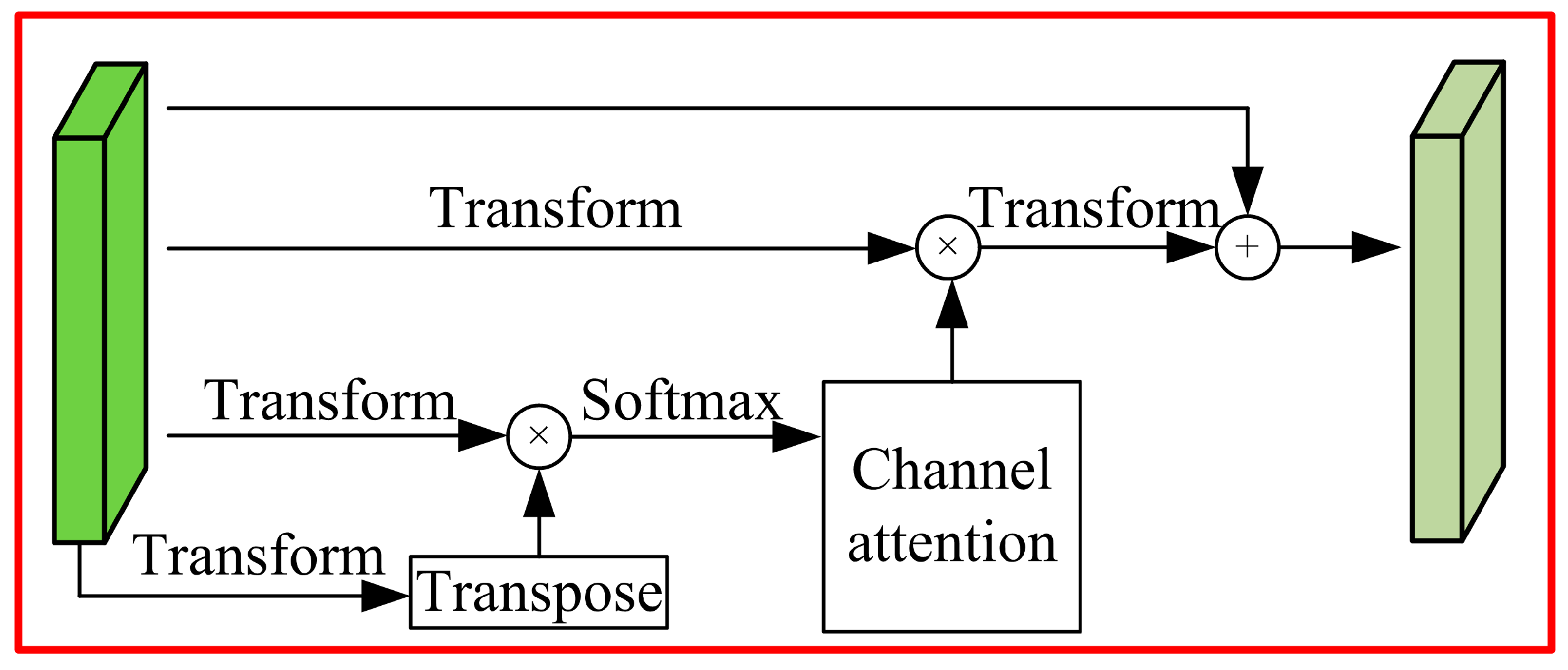
Channel attention mechanism module: high-level semantic features of different channels are extracted to achieve category forecast, and there is a certain relationship between the different categories of semantic. By using the contact between different channel feature images, the feature images that are interconnected can be highlighted, and specific semantic features can be promoted, so it is necessary to explore the features of the different channels. The channel attention module is shown in Figure 4.

The channel attention module can directly obtain the attention diagram through matrix A:

$$x_{ji}=\frac{\exp \left[{A^{\prime }}_i\cdot {\left(A^{\prime }\right)}_j^T\right]}{{\displaystyle \sum _{i=1}^C\exp \left[{A^{\prime }}_i\cdot {\left(A^{\prime }\right)}_j^T\right]}}$$

(9)

The corresponding channel attention is:

$$E_{channel}^j=\beta {\displaystyle \sum _{i=1}^C\left(x_{ji}|A_i\right)+A_j}$$

(10)

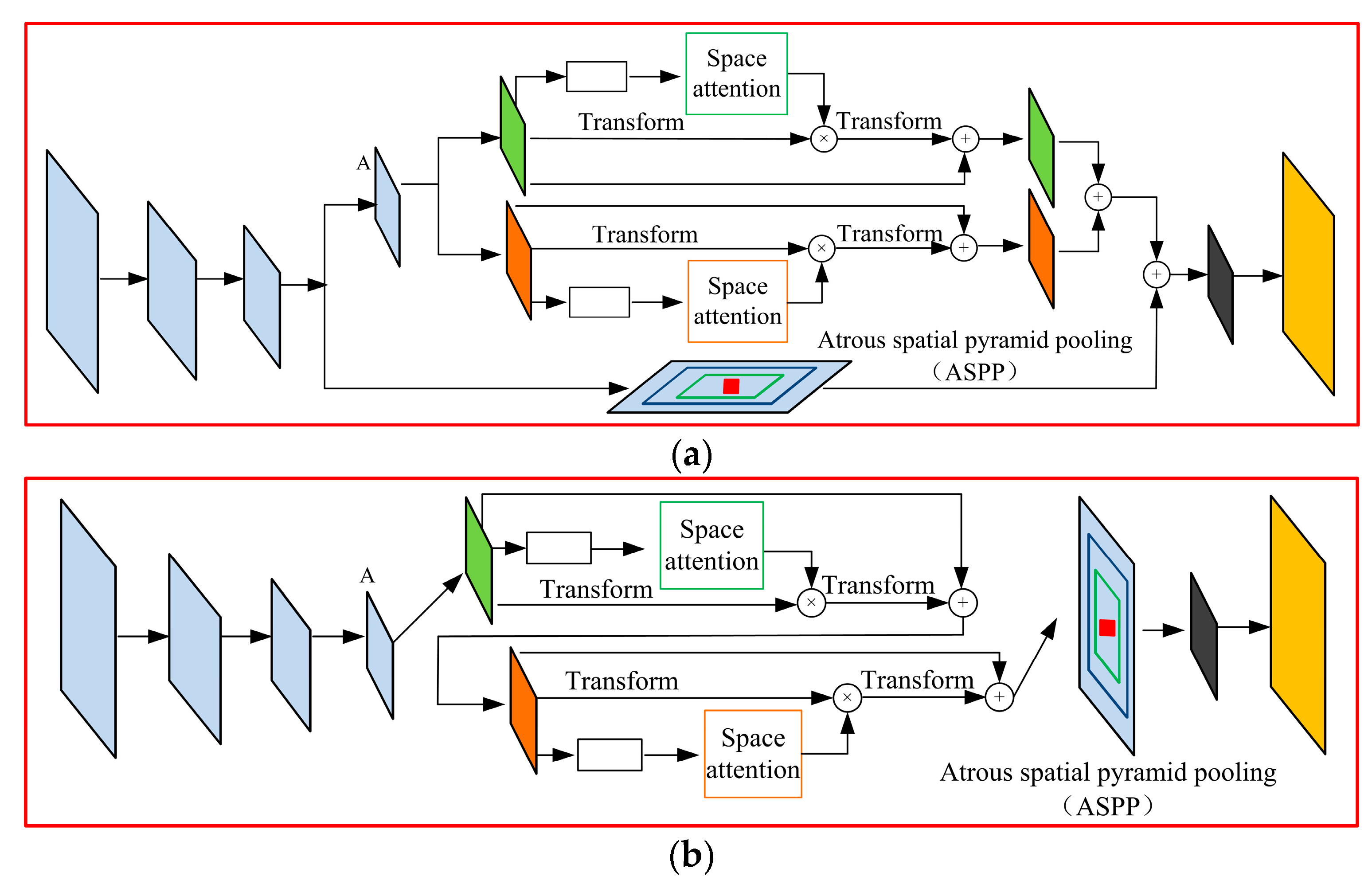
where β is the learning parameter, and each channel feature is the weighted sum of all channel features and the original channel features, so the channel attention module can simulate the long-term semantic dependence between different feature maps to enhance feature representation. Based on the above analysis, the Deeplabv3+ model of double attention mechanism is proposed, and the network structure is shown in Figure 5.

Figure 5a shows the parallel network of DAMM and ASPP. The trunk network is used to extract image features, two branch networks are adopted to process the feature images extracted from the backbone network, and then the two branch feature images are fused. The upper branch in the figure is a dual attention mechanism module (channel attention and spatial attention). The two modules operate in parallel in the dual attention module. The feature images extracted from the backbone network are convolved with a dilation rate of 2 and a convolution kernel of 3 × 3, and then sent to the channel attention module and the location attention module for processing, respectively, and the feature images are summed. The channel attention module uses the correlation between the relevant category features of different channels to strengthen different category features and improve the classification accuracy, while the spatial attention module promotes the classification accuracy of different local features by simulating the connection between different local features. The lower branch fuses the feature image processed by ASPP with the feature image processed by the dual attention module, and finally reduces the dimension of the fusion feature image. The network decoding module adopts the DeepLabv3+ decoding module to operate, and finally, the image segmentation map is obtained.

Figure 5b shows the series network of DAMM and ASPP. It uses the trunk network to extract feature images, and the feature images are convolved with an expansion rate of 2 and a convolution kernel of 3 × 3. The results are sent into DAMM for spatial and inter-channel pixel feature enhancement of feature images and then input into the ASPP module for multi-scale target segmentation. Finally, the decoding and restoration of the feature map are carried out according to the original network method.

2.4. Segmentation Model Based on HRNet

To improve the accuracy of coastline extraction, an enhanced network segmentation model based on depth discrimination is proposed. It mainly includes data preprocessing, depth feature extraction, similarity calculation, and loss minimization function calculation. The output of the lth layer of the convolutional neural network is z_l, and {H_l, W_l, C_l} is the feature resolution.

HRNet is adopted to achieve feature extraction, and the structure is shown in Figure 6. HRNet consists of four network branches that are used to extract features of different scales. In the last layer, multi-scale features are superimposed and fused, and the basic structure of HRNet consists of a convolution layer and an upsampling layer.

For the l-th convolutional network, its input data is z_l−1, and then the corresponding convolution expression is:

$$a=f\left(Z_{l-1}\ast W+b\right)$$

(11)

where f(.) is a nonlinear corresponding function, and if the moving step of the convolution kernel reduces the spatial dimension of the data in the process of feature extraction, upsampling is used to expand the spatial dimension of the feature map to make the feature map and the original input image have the same spatial scale. HRNet uses bilinear differences to restore the spatial dimensions of feature maps. The convolutional neural network obtains the depth feature vector corresponding to each pixel layer by layer and through superposing convolutional layer, up-sampling layer, and other networks. Softmax is used to classify the extracted features. It is assumed that the convolutional neural network adopted has a total of L layers, and then the l-th layer network is classifier Softmax:

$$p\left(n|z_{0,i}\right)=\frac{\exp \left(w_{L,n}•z_{L-1,i}\right)}{{\displaystyle \sum _{c=1}^n\exp \left(w_{L,c}•z_{L-1,i}\right)}}$$

(12)

where z_0,i is the i-th pixel of the input image, and p(k|z_0,i) represents the probability that sample pixel z_0,i belongs to the k class. The essence of Softmax process can be regarded as similarity calculation, which calculates the inner product of feature vector z_L−1,i of pixel z_0,i as the similarity to judge the membership degree of pixel z_0,i. Therefore, the parameter vector w_L,c of each class can be regarded as the corresponding category center of this class. When the modules of the parameter vectors of each category are equal, the inner product similarity between the depth features of the pixel to be classified and the category center is transformed into the included angle between the high-dimensional depth features of the comparison pixel and the category center of each category, that is, the category of the pixel to be classified is judged by calculating the included angle between the depth features of the pixel to be classified and the category center. 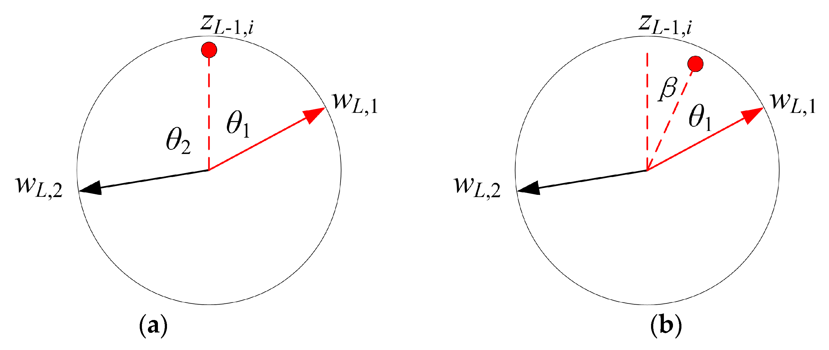Because the angle θ_i,1 between feature point z_L−1,i and category center w_L,1 is the smallest, pixel z_0,i is divided into class 1. At this point, Softmax is transformed into:

$$p\left(n|z_{0,i}\right)=\frac{\exp \left(S_q\cos \left({\theta }_{n,i}\right)\right)}{{\displaystyle \sum _{c=1}^n\exp \left(S_q\cos \left({\theta }_{c,i}\right)\right)}}$$

(13)

$$Sq=\left|w_{L,t}\right|•\left|z_{L-1,i}\right|$$

(14)

Therefore, to increase the distinctiveness of depth features and make the depth features of similar pixels get to its corresponding category center, the included angle between category center w_L,c in the Softmax and depth features of pixels is taken as a similarity for measurement, and then the punishment factor β is added to make the training sample and its corresponding category center have a smaller angle in the training stage. The corresponding included angle is:

θ_t,I = arcos(w_L,t·z_l−1,i)

(15)

For any pixel z_0,i, assuming its category is t, then its probability of belonging to class t is:

$$p\left(t|z_{0,i}\right)=\frac{\exp \left(S_q\cos \left({\theta }_{n,i}+\beta \right)\right)}{\exp \left(S_q\cos \left({\theta }_{n,i}+\beta \right)\right)+{\displaystyle \sum _{c=1}^n\exp \left(S_q\cos \left({\theta }_{c,i}\right)\right)}}$$

(16)

In the loss calculation stage, the classification probability is maximized according to the maximum likelihood rule, and the classification loss function is obtained:

$$J=-\frac{1}{m}{\displaystyle \sum _{i=1}^m\lg p\left(y_i|z_{0,i}\right)}$$

(17)

where m is the number of trained pixel samples; y_i is the category of pixel i. When J takes the minimum value, it forces the sample to move to the center of its category, making the included angle smaller to compensate for the angle increase caused by the penalty factor β. By comparing Figure 7a,b, it can be seen that traditional Softmax and improved Softmax are used to calculate the probability that z_0,i belongs to class l. When the two get the same probability, the included angle between pixel z_0,i and class center w_L,1 in Figure 7b is smaller than that in Figure 7a. Therefore, in the training stage, the feature of the pixel sample is made to get close to its corresponding category center.

In the training stage, network parameters are updated by alternatively carrying out forward and backward operations. In the backward stage, the gradient descent algorithm is adopted to update network parameters:

$$w=w-\lambda \frac{\partial L}{\partial w}$$

(18)

where w represents the parameters of each layer in the convolutional neural network; λ is the learning rate, which is used to control the step length of network parameter update.

2.5. Coastline Recognition Algorithm Based on Image Straightening

Based on the above introduction, we have obtained the segmentation algorithms of the two models, which need to be fused. Currently, the main fusion methods are: pixel-level image fusion, feature set fusion, and decision set fusion [70].

Pixel-level image fusion directly fuses the pixel points of the image. The scale of original image data results in time-consuming algorithm implementation. Without data processing, the advantages and disadvantages of the original sensor information will overlay and affect the fusion effect. The requirements of hardware facilities are quite high. When carrying out image fusion, the accuracy requires to be each pixel of the sensor data; As it is based on pixel calculation, pixel information is susceptible to pollution, noise, and other interference, so the effect is not stable.

Feature-level fusion is a process in which edge, shape, contour, local feature, and other information are synthetically processed after feature extraction. Feature-level fusion includes target state information fusion and target characteristic fusion. Feature level fusion includes several modules: source image acquisition, image preprocessing, image segmentation, feature extraction, feature data fusion, and target recognition. The feature fusion of an image is a kind of cost processing, which reduces the amount of data, retains most of the information, and still loses part of the details. The combination of original features form features, increases the dimension of features, and improves the accuracy of the target. Feature vectors can be directly fused or recombined according to the attributes of features themselves, and edge, shape, and clearance light are all important parameters to describe features. Target state feature fusion is a kind of target statistical feature based on multi-scale and multi-resolution, and it extracts and describes the original data state of the image and requires strict registration, and an image containing more image information can be obtained ultimately. It conducts statistics of state information of an image and then performs pattern matching. Its core idea is to achieve accurate state estimation of multi-sensor targets, and it is effectively associated with prior knowledge, so it is widely used in target tracking. The target feature fusion is the internal description of the feature extracted from the image features according to the specific semantics, or the recombination of feature attributes. These feature vectors represent abstract image information, and the features are directly recognized by machine learning theory fusion, which increases the dimension of features and improves the accuracy of target recognition. Target feature fusion is feature vector fusion recognition, which generally deals with high-dimensional problems. In essence, the fusion application is mostly pattern recognition. Compared with a single sensor, the information provided by a multi-sensor increases the dimension of feature space and enlarges the space of fine information feature scattering.

Decision-level fusion: on the basis of each sensor independently completing the decision or classification, the recognition results of multiple sensors are fused to make the global optimal decision. According to certain rules, the decision-level fusion can synthesize the source image after feature extraction and recognition and then obtain the fusion image. The input of the decision is the cognitive framework of the target. The recognition framework is formed after the basic processing of preprocessing, feature extraction and recognition by observing the target in the same scene through homogeneous and heterogeneous sensors. The fusion result is obtained by optimization decision. The decision-level fusion tends to be intelligent logic, and the recognition result of the integrated multi-sensor is more accurate and effective than single recognition. The advantages of the decision-level fusion are as follows: it has good real-time performance and self-adaptability, low data requirements and strong anti-interference ability; it is able to efficiently be compatible with multi-sensor environmental characteristic information; it has good error correction ability; it can eliminate the error caused by a single sensor through proper fusion; and the system can also obtain correct results.

As there are certain rules for the environment around the coastline, we firstly fuse the decision sets of the dual-attention network and HRnet network mentioned above, and then set thresholds to constrain pixel attributes. Let the probability that the pixel point (x,y) extracted by the dual attention network is a coastline be P₁(x,y) and the probability that the pixel point (x,y) extracted by the HRnet network is a coastline be P₂(x,y). P = (P₁(x,y) + P₂(x,y))/2 and set a threshold T to constrain the pixel properties, which is chosen to be 0.6 in this paper. Secondly, with the coastline as the center and D as the width, the image data around the center line are obtained, and these data are straightened out to visually display and analyze image data as show Figure 8. The areas belonging to the coastline are retained and others are removed.

3. Experiment Analysis

The multi-spectral data is taken by Ziyuan 3 satellite, including Sri Lanka data in four bands. Linux system, image server, seven 12G graphics cards driver version 430.64, CUDA 10.1, and Python loaded deep learning framework were used to carry out the research.

The island of Sri Lanka is roughly pear-shaped, as shown in Figure 9. Its central and southern parts are plateaus, of which the Pidulu Talagra Mountain is 2524 m above sea level, the highest point in the country. The northern and coastal areas are plains, of which the northern coastal plain is wide, and the southern and western coastal plains are relatively narrow, with an elevation of 150 m. There are a large number of rivers in Sri Lanka, with 16 main rivers, most of which originate in the central mountainous area, with short river basin, rapid flow, as well as very abundant water flow. The longest river is the Mahaweli, which is 335 km long and flows into the Indian Ocean near the Port of Trincomalee. There are scattered lakes in the eastern plain, among which Batticalo Lake is the largest, with an area of 120 square kilometers. Therefore, in this study, the representative remote sensing images are selected for experiments, as shown in Figure 10.

3.1. Introduction to Evaluation Indicators

To verify the performance of the image quality algorithm, image quality is evaluated from the objective dimension. AG is the mean gradient, SD is the standard deviation, SF is the spatial frequency, and EI is the edge intensity.

$$\{\begin{array}{l}AG=\frac{1}{\left(M-1\right)\left(N-1\right)}{\displaystyle \sum _{i=1}^{M-1}{\displaystyle \sum _{j=1}^{N-1}\sqrt{\frac{{\left(I_{i+1,j}-I_{i,j}\right)}^2+{\left(I_{i,j+1}-I_{i,j}\right)}^2}{2}}}}\\ SD=\frac{\sqrt{{\displaystyle \sum _{i=1}^M{\displaystyle \sum _{j=1}^N{\left(I_{i,j}-\mu \right)}^2}}}}{MN}\\ SF=\sqrt{\frac{{\displaystyle \sum _{i=1}^M{\displaystyle \sum _{j=2}^N{\left(I_{i,j}-I_{i,j-1}\right)}^2}}+{\displaystyle \sum _{i=2}^M{\displaystyle \sum _{j=1}^N{\left(I_{i,j}-I_{i-1,j}\right)}^2}}}{MN}}\\ EI=\frac{\sqrt{{\displaystyle \sum _{i=1}^M{\displaystyle \sum _{j=1}^N\left[s_x{\left(i,j\right)}^2+s_y{\left(i,j\right)}^2\right]}}}}{MN}\end{array}$$

(19)

To verify the image segmentation effect, we introduce evaluation indexes such as AOM, AVM, AUM, and CM to demonstrate the performance of the algorithm [71].

$$\{\begin{array}{l}AOM=\frac{R_s\cap R_g}{R_s\cup R_g}\\ AVM=\frac{R_s-R_g}{R_s}\\ AUM=\frac{R_g-R_s}{R_g}\\ CM=\frac{1}{3}\left\{AOM+\left(1-AVM\right)+\left(1-AUM\right)\right\}\end{array}$$

(20)

where R_g is the gold standard and R_s is the segmentation result of the algorithm. AOM and CM are directly proportional to the algorithm performance, while AVM and AUM are inversely proportional to the algorithm performance.

To verify the network performance, the MIOU (Mean Intersection over Union) is introduced to measure the convergence of the algorithm [72]:

$$MIoU=\frac{1}{k+1}{\displaystyle \sum _{i=0}^k\frac{p_{ii}}{{\displaystyle \sum _{j=0}^k{p}_{ij}+{\displaystyle \sum _{j=0}^k{p}_{ji}-p_{ii}}}}}$$

(21)

3.2. Image Enhancement

The original image contains large noise, and the overall image is dark. The histogram algorithm [23] redistributes the pixel values to enhance the pixel values of the dark part and reduce the pixel values of the contest part, thus improving the overall performance of the image. The Gaussian algorithm [61] filters the image and realizes the image enhancement, and the image is smooth. As shown in Figure 11a, the short coastline image includes clouds (3%), ground objects (88%), and oceans (9%). As shown in

Table 1. Short coastline image quality.

Algorithm	AG	SD	SF	IE
Original	8.7	46.3	34.2	5.1
Histogram	9.1	56.6	35.3	6.3
Gaussian filter	8.8	48.1	47.1	5.6
Ours	10.1	58.3	48.5	7.1

, the ground objects are abundant. The algorithm highlights the detailed features of the image, and the histogram algorithm constructs the mapping to achieve image enhancement. The model constructed by the Gaussian filtering algorithm has an obvious effect on image smoothing. As shown in Figure 11b, the long coastline image includes clouds (6%), ground objects (40%), and oceans (54%). As shown in

Table 2. Long coastline image quality.

Algorithm	AG	SD	SF	IE
Original	8.5	44.1	35.1	4.8
Histogram	9.3	58.3	34.2	6.0
Gaussian filter	9.1	49.2	48.5	5.3
Ours	9.9	59.4	49.3	6.9

, there are more features, oceans, and clouds in the highlighted area, and the algorithm performance is reduced to a certain extent. As shown in Figure 11c, multi-coastline images include clouds (8%), ground objects (72%), and oceans (20%). As shown in

Table 3. Multiple coastlines image quality.

Algorithm	AG	SD	SF	IE
Original	8.3	45.2	33.1	4.5
Histogram	8.5	51.2	34.3	6.1
Gaussian filter	8.3	46.2	46.3	5.4
Ours	9.5	54.3	47.2	6.5

, due to the influence of shooting direction and clouds, the coastline shows two sections, and the algorithm effect is reduced. As shown in Figure 11d, the cloud-shielded coastline image includes thin clouds (8%), ground objects (80%), and oceans (10%). As shown in

Table 4. Cloud shielded coastline image quality.

Algorithm	AG	SD	SF	IE
Original	7.9	41.3	36.3	4.2
Histogram	8.5	52.4	31.5	5.4
Gaussian filter	8.1	48.5	42.1	5.7
Ours	9.3	51.8	46.3	6.1

, as the whole image is blurred due to the influence of thin clouds, the improvement of all algorithms is limited. Through the image comparison effect, it can be seen that the PCA constructed in this paper can extract the principal components of the image and suppress the noise, showing good results in vision and indicators.

3.3. Attention Network Experiment

We proposed the dual attention network, which has series and parallel structures. Therefore, we compared the Deeplabv3+ with series and parallel networks. In general, the network based on Deeplabv3+ can realize coastline identification, and with the deepening of the network structure, the identification effect shows an upward trend. Both series and parallel dual attention mechanisms mentioned in this paper improve the performance of the algorithm. The parallel network extracts spatial information and channel information and integrates them through different branches to improve algorithm performance. As shown in

Table 5. Short coastline extraction effect.

Algorithm	Number of Basic Network Layers	AOM	AVM	AUM	CM
Deeplabv3+	16	0.85	0.24	0.22	0.80
Deeplabv3+	32	0.91	0.21	0.19	0.84
In series	32	0.93	0.18	0.16	0.86
In parallel	32	0.95	0.16	0.14	0.88

, the coastline is short, and the extraction accuracy is the highest. As shown in

Table 6. Long coastline extraction effect.

Algorithm	Number of Basic Network Layers	AOM	AVM	AUM	CM
Deeplabv3+	16	0.78	0.33	0.31	0.71
Deeplabv3+	32	0.81	0.31	0.26	0.75
In series	32	0.84	0.27	0.23	0.78
In parallel	32	0.90	0.25	0.18	0.82

, with the increase of the coastline length, the accuracy of the algorithm decreases. The parallel performance can still reach 0.90. As shown in

Table 7. Multiple coastlines extraction effect.

Algorithm	Number of Basic Network Layers	AOM	AVM	AUM	CM
Deeplabv3+	16	0.72	0.35	0.29	0.69
Deeplabv3+	32	0.78	0.32	0.24	0.74
In series	32	0.83	0.28	0.23	0.77
In parallel	32	0.88	0.24	0.19	0.82

, an image contains two coastal regions, and the influence of thick clouds increases the difficulty of algorithm recognition, resulting in a significant decrease in the algorithm effect. As shown in

Table 8. Cloud sheltered coastline extraction effect.

Algorithm	Number of Basic Network Layers	AOM	AVM	AUM	CM
Deeplabv3+	16	0.83	0.29	0.25	0.76
Deeplabv3+	32	0.86	0.26	0.21	0.80
In series	32	0.90	0.22	0.19	0.83
In parallel	32	0.93	0.19	0.16	0.86

, the whole image is blurred due to the influence of thin clouds, but the coastline is short, so it can be better identified by the parallel form of Deeplabv3+, which proves the effectiveness of the algorithm. As can be seen from Figure 12, the attention network responds strongly in the region where the ocean is located, realizing the distinction between marine and land surface features. However, some objects are still incorrectly identified, which will be further removed by the subsequent algorithm. Based on the above analysis, this paper will adopt the parallel method to carry out follow-up research.

As shown in Figure 13, as the DeepLabv3+ network is relatively deep, there is instability and slow training during training. The algorithm proposed in this paper constructs an attention model from the perspective of space and channel. The serial attention model reaches 84% when it is stable, and the parallel attention model reaches 86%. Based on the above analysis, it can be seen that the parallel attention model has stronger stability. Therefore, in the subsequent experiments, we will adopt the parallel attention model structure.

3.4. HRNet Network Experiment

In the HRNet network, parameter β determines the degree to which pixel features get close to their category center, which determines the discrimination of features. β = [0.1, 1] is selected for analysis, and kapa coefficient is calculated under different values of β. As shown in Figure 14, the segmentation accuracy is improved in the process that β increases from 0.1 to 0.5, and the optimal value is obtained when β = 0.5. Later, with the continuous increase of β, the segmentation accuracy decreases. Therefore, our follow-up study will be carried out when β = 0.5. The extraction effect of HRnet is shown in Figure 15. Then, the loss function is modified to obtain the classification effect of seawater and other substances.

3.5. Coastline Extraction Effect Display

To visually display the effect of the algorithm, we take the coastline as the center and the adjacent 600 pixels as the range to straighten the image, as shown in Figure 16a. Due to the short coastline, it is less affected, and the straightening effect is the best. The upper and lower parts of the image show the land and ocean areas, respectively. As shown in Figure 16b, due to the long coastline and the occlusion in the cloud area above the image, some coastlines in the cloud cannot be extracted. Coupled with the long coastline, the phenomenon of image blur occurs during mapping. According to Figure 16c, the coastline is divided into three sections due to image capture and cloud occlusion, which are shown in red, green, and yellow. As shown in Figure 16d, the image is blurred as a whole, and there are wave images on the coastline, making the segmentation effect fluctuate. However, in general, the algorithm we constructed realizes the extraction of coastline from the perspective of image enhancement, dual attention network recognition, Hrnet network recognition, and decision set fusion, so it has a good effect.

4. Conclusions

In the face of the actual demand for coastline extraction and the problem of difficult coastline recognition, we established models from the perspective of image enhancement, dual attention network recognition, and HRENT network construction, and realized coastline extraction through the fusion idea of decision sets. Experiments show that the proposed algorithm accurately focused on the difference between sea and land to build a coastline straightening model, aiming to realize the intuitive display of the coastline. The specific innovations can be summarized as follows: (1) a PCA image enhancement algorithm was proposed based on remote sensing image features; (2) the spatial attention and channel attention models were proposed, and suspected regions were extracted from parallel and series perspectives; and (3) the improved Softmax function improved HRENT network performance. The idea of decision set fusion was adopted to realize coastline extraction, and a coastline straightening algorithm was proposed to intuitively display the effect.

However, in the research process, there are still the following problems: (1) remote sensing images have high resolution, and still take a lot of time during training and testing, which cannot meet the requirements of real-time detection; (2) the decision set fusion method currently adopted relies on the same group of data to carry out the training of dual attention network and HRENT network, and further studies are needed to determine if the algorithm is extensible; and (3) in the process of image straightening, due to the vertical angle problem, there is the problem of insufficient spatial resolution in the sampling process, resulting in poor visual effects or blurred images, so we will carry out further studies based on the above issues.

References

1. Gervais, C.; Champion, C.; Pecl, G.T. Species on the move around the Australian coastline: A continental-scale review of climate-driven species redistribution in marine systems. Glob. Change Biol. 2021, 27, 3200–3217. [Google Scholar] [CrossRef]
2. Chen, S.; Tang, Y.; Zou, X.; Huo, H.; Hu, K.; Hu, B.; Pan, Y. Identification and detection of biological information on tiny biological targets based on subtle differences. Machines 2022, 10, 996. [Google Scholar] [CrossRef]
3. Wang, X.; Yan, F.; Su, F. Changes in coastline and coastal reclamation in the three most developed areas of China, 1980–2018. Ocean Coast. Manag. 2021, 204, 105542. [Google Scholar] [CrossRef]
4. Wang, P.; Bayram, B.; Sertel, E. A comprehensive review on deep learning based remote sensing image super-resolution methods. Earth Sci. Rev. 2022, 232, 104110. [Google Scholar] [CrossRef]
5. Zhang, D.; Zhao, J.; Chen, J.; Zhou, Y.; Shi, B.; Yao, R. Edge-aware and spectral-spatial information aggregation network for multispectral image semantic segmentation. Eng. Appl. Artif. Intell. 2022, 114, 105070. [Google Scholar] [CrossRef]
6. Yao, D.; Zhi-li, Z.; Xiao-feng, Z.; Wei, C.; Fang, H.; Yao-ming, C.; Cai, W.W. Deep hybrid: Multi-graph neural network collaboration for hyperspectral image classification. Def. Technol. 2022, in press. [CrossRef]
7. Bai, X.; Zhou, F.; Xue, B. Image enhancement using multi scale image features extracted by top-hat transform. Opt. Laser Technol. 2012, 44, 328–336. [Google Scholar] [CrossRef]
8. Rubel, A.; Lukin, V.; Uss, M.; Vozel, B.; Pogrebnyak, O.; Egiazarian, K. Efficiency of texture image enhancement by DCT-based filtering. Neurocomputing 2016, 175, 948–965. [Google Scholar] [CrossRef] [Green Version]
9. Lee, E.; Kim, S.; Kang, W.; Seo, D.; Paik, J. Contrast enhancement using dominant brightness level analysis and adaptive intensity transformation for remote sensing images. IEEE Geosci. Remote Sens. Lett. 2012, 10, 62–66. [Google Scholar] [CrossRef]
10. Fu, X.; Liao, Y.; Zeng, D.; Huang, Y.; Zhang, X.P.; Ding, X. A probabilistic method for image enhancement with simultaneous illumination and reflectance estimation. IEEE Trans. Image Process. 2015, 24, 4965–4977. [Google Scholar] [CrossRef] [PubMed]
11. Zhong, S.; Jiang, X.; Wei, J.; Wei, Z. Image enhancement based on wavelet transformation and pseudo-color coding with phase-modulated image density processing. Infrared Phys. Technol. 2013, 58, 56–63. [Google Scholar] [CrossRef]
12. Wang, M.; Zheng, X.; Feng, C. Color constancy enhancement for multi-spectral remote sensing images. In Proceedings of the 2013 IEEE International Geoscience and Remote Sensing Symposium-IGARSS, Melbourne, VIC, Australia, 21–26 July 2013; IEEE: Piscataway, NJ, USA, 2013; pp. 864–867. [Google Scholar]
13. Wong, C.Y.; Jiang, G.; Rahman, M.A.; Liu, S.; Lin, S.C.F.; Kwok, N.; Wu, T. Histogram equalization and optimal profile compression based approach for colour image enhancement. J. Vis. Commun. Image Represent. 2016, 201638, 802–813. [Google Scholar] [CrossRef]
14. Li, J. Application of image enhancement method for digital images based on Retinex theory. Optik 2013, 124, 5986–5988. [Google Scholar] [CrossRef]
15. Rubel, A.; Naumenko, A.; Lukin, V. A neural network based predictor of filtering efficiency for image enhancement. In Proceedings of the 2014 IEEE Microwaves, Radar and Remote Sensing Symposium (MRRS), Kiev, Ukraine, 23–25 September 2014; IEEE: Piscataway, NJ, USA, 2014; pp. 14–17. [Google Scholar]
16. Li, L.; Si, Y.; Jia, Z. Remote sensing image enhancement based on non-local means filter in NSCT domain. Algorithms 2017, 10, 116. [Google Scholar] [CrossRef] [Green Version]
17. Huang, Z.; Fang, H.; Li, Q.; Li, Z.; Zhang, T.; Sang, N.; Li, Y. Optical remote sensing image enhancement with weak structure preservation via spatially adaptive gamma correction. Infrared Phys. Technol. 2018, 94, 38–47. [Google Scholar] [CrossRef]
18. Park, S.; Yu, S.; Moon, B.; Ko, S.; Paik, J. Low-light image enhancement using variational optimization-based retinex model. IEEE Trans. Consum. Electron. 2017, 63, 178–184. [Google Scholar] [CrossRef]
19. Pathak, S.S.; Dahiwale, P.; Padole, G. A combined effect of local and global method for contrast image enhancement. In Proceedings of the 2015 IEEE International Conference on Engineering and Technology (ICETECH), Coimbatore, India, 20 March 2015; IEEE: Piscataway, NJ, USA, 2015; pp. 1–5. [Google Scholar]
20. Agrawal, S.; Panda, R. An efficient algorithm for gray level image enhancement using cuckoo search. In Proceedings of the International Conference on Swarm, Evolutionary, and Memetic Computing, Bhubaneswar, India, 20–22 December 2012; Springer: Berlin/Heidelberg, Germany, 2012; pp. 82–89. [Google Scholar]
21. Riaz, M.M.; Ghafoor, A. Principle component analysis and fuzzy logic based through wall image enhancement. Prog. Electromagn. Res. 2012, 127, 461–478. [Google Scholar] [CrossRef] [Green Version]
22. Liejun, W.; Ting, Y. A new approach of image enhancement based on improved fuzzy domain algorithm. In Proceedings of the 2014 International Conference on Multisensor Fusion and Information Integration for Intelligent Systems (MFI), Beijing, China, 28–29 September 2014; IEEE: Piscataway, NJ, USA, 2014; pp. 1–5. [Google Scholar]
23. Muniyappan, S.; Allirani, A.; Saraswathi, S. A novel approach for image enhancement by using contrast limited adaptive histogram equalization method. In Proceedings of the 2013 4th International Conference on Computing, Communications and Networking Technologies (ICCCNT), Tiruchengode, India, 4–6 July 2013; pp. 1–6. [Google Scholar]
24. Fu, X.; Wang, J.; Zeng, D.; Huang, Y.; Ding, X. Remote sensing image enhancement using regularized-histogram equalization and DCT. IEEE Geosci. Remote Sens. Lett. 2015, 12, 2301–2305. [Google Scholar] [CrossRef]
25. Abramova, V.V.; Abramov, S.K.; Lukin, V.V.; Egiazarian, K.O.; Astola, J.T. On required accuracy of mixed noise parameter estimation for image enhancement via denoising. EURASIP J. Image Video Process. 2014, 1, 3. [Google Scholar] [CrossRef] [Green Version]
26. Bhandari, A.K.; Maurya, S.; Meena, A.K. Social spider optimization based optimally weighted Otsu thresholding for image enhancement. IEEE J. Sel. Top. Appl. Earth Obs. Remote Sens. 2018, 1–13. [Google Scholar] [CrossRef]
27. Somvanshi, S.S.; Kunwar, P.; Tomar, S.; Singh, M. Comparative statistical analysis of the quality of image enhancement techniques. Int. J. Image Data Fusion 2018, 9, 131–151. [Google Scholar] [CrossRef]
28. Md Noor, S.S.; Michael, K.; Marshall, S.; Ren, J. Hyperspectral image enhancement and mixture deep-learning classification of corneal epithelium injuries. Sensors 2017, 17, 2644. [Google Scholar] [CrossRef] [PubMed] [Green Version]
29. Ramkumar, G.; Ayyadurai, M.; Senthilkumar, C. An effectual underwater image enhancement using deep learning algorithm. In Proceedings of the 2021 5th International Conference on Intelligent Computing and Control Systems (ICICCS), Madurai, India, 6–8 May 2021; IEEE: Piscataway, NJ, USA, 2021; pp. 1507–1511. [Google Scholar]
30. Park, S.; Yu, S.; Kim, M.; Park, K.; Paik, J. Dual autoencoder network for retinex-based low-light image enhancement. IEEE Access 2018, 6, 22084–22093. [Google Scholar] [CrossRef]
31. Jiang, K.; Wang, Z.; Yi, P.; Wang, G.; Lu, T.; Jiang, J. Edge-enhanced GAN for remote sensing image superresolution. IEEE Trans. Geosci. Remote Sens. 2019, 57, 5799–5812. [Google Scholar] [CrossRef]
32. Munadi, K.; Muchtar, K.; Maulina, N.; Pradhan, B. Image enhancement for tuberculosis detection using deep learning. IEEE Access 2020, 8, 217897–217907. [Google Scholar] [CrossRef]
33. Kuang, X.; Sui, X.; Liu, Y.; Chen, Q.; Gu, G. Single infrared image enhancement using a deep convolutional neural network. Neurocomputing 2019, 332, 119–128. [Google Scholar] [CrossRef]
34. Guo, Y.; Zhou, M.; Wang, Y.; Wu, G.; Shibasaki, R. Learn to Be Clear and Colorful: An End-to-End Network for Panchromatic Image Enhancement. IEEE Geosci. Remote Sens. Lett. 2022, 19, 1–5. [Google Scholar] [CrossRef]
35. Zheng, C.; Wang, L.; Chen, R.; Chen, X. Image segmentation using multiregion-resolution MRF model. IEEE Geosci. Remote Sens. Lett. 2012, 10, 816–820. [Google Scholar] [CrossRef]
36. Miaozhong, X.; Ming, C.; Lijuan, W.; Tianpeng, X.; Xiaoling, Z. A methodology of image segmentation for high resolution remote sensing image based on visual system and Markov random field. Acta Geod. Cartogr. Sin. 2015, 44, 198. [Google Scholar]
37. Ming, D.; Ci, T.; Cai, H.; Li, L.; Qiao, C.; Du, J. Semivariogram-based spatial bandwidth selection for remote sensing image segmentation with mean-shift algorithm. IEEE Geosci. Remote Sens. Lett. 2012, 9, 813–817. [Google Scholar] [CrossRef]
38. Deng, C.; Li, S.; Bian, F.; Yang, Y. Remote sensing image segmentation based on mean shift algorithm with adaptive bandwidth. In Proceedings of the International Conference on Geo-Informatics in Resource Management and Sustainable Ecosystem, Ypsilanti, MI, USA, 3–5 October 2014; Springer: Berlin/Heidelberg, Germany, 2014; pp. 179–185. [Google Scholar]
39. Yuan, J.; Wang, D.; Li, R. Remote sensing image segmentation by combining spectral and texture features. IEEE Trans. Geosci. Remote Sens. 2013, 52, 16–24. [Google Scholar] [CrossRef]
40. Liu, S.; Luk, W. Towards an efficient accelerator for DNN-based remote sensing image segmentation on FPGAs. In Proceedings of the 2019 29th International Conference on Field Programmable Logic and Applications (FPL), Barcelona, Spain, 8–12 September 2019; IEEE: Piscataway, NJ, USA, 2019; pp. 187–193. [Google Scholar]
41. Li, N.; Huo, H.; Zhao, Y.M.; Chen, X.; Fang, T. A spatial clustering method with edge weighting for image segmentation. IEEE Geosci. Remote Sens. Lett. 2013, 10, 1124–1128. [Google Scholar]
42. Fang, L.; Wang, X.; Sun, Y.; Xu, K. Remote sensing image segmentation using active contours based on intercorrelation of nonsubsampled contourlet coefficients. J. Electron. Imaging 2016, 25, 061405. [Google Scholar] [CrossRef]
43. Huang, Z.; Zhang, J.; Li, X.; Zhang, H. Remote sensing image segmentation based on dynamic statistical region merging. Optik 2014, 125, 870–875. [Google Scholar] [CrossRef]
44. Wang, Y.; Qi, Q.; Liu, Y.; Jiang, L.; Wang, J. Unsupervised segmentation parameter selection using the local spatial statistics for remote sensing image segmentation. Int. J. Appl. Earth Obs. Geoinf. 2019, 81, 98–109. [Google Scholar] [CrossRef]
45. Yang, Y.; Li, H.T.; Han, Y.S.; Gu, H.Y. High resolution remote sensing image segmentation based on graph theory and fractal net evolution approach. Int. Arch. Photogramm. Remote Sens. Spat. Inf. Sci. 2015, 40, 197. [Google Scholar] [CrossRef] [Green Version]
46. Zhang, C.; Li, G.; Du, S. Multi-scale dense networks for hyperspectral remote sensing image classification. IEEE Trans. Geosci. Remote Sens. 2019, 57, 9201–9222. [Google Scholar] [CrossRef]
47. Yang, J.; He, Y.; Caspersen, J. A self-adapted threshold-based region merging method for remote sensing image segmentation. In Proceedings of the 2016 IEEE International Geoscience and Remote Sensing Symposium (IGARSS), Beijing, China, 10–15 July 2016; IEEE: Piscataway, NJ, USA, 2016; pp. 6320–6323. [Google Scholar]
48. He, P.; Shi, W.; Zhang, H.; Hao, M. A novel dynamic threshold method for unsupervised change detection from remotely sensed images. Remote Sens. Lett. 2014, 5, 396–403. [Google Scholar] [CrossRef]
49. Basaeed, E.; Bhaskar, H.; Al-Mualla, M. Supervised remote sensing image segmentation using boosted convolutional neural networks. Knowl. Based Syst. 2016, 99, 19–27. [Google Scholar] [CrossRef]
50. Alam, F.I.; Zhou, J.; Liew, A.W.C.; Jia, X. CRF learning with CNN features for hyperspectral image segmentation. In Proceedings of the 2016 IEEE International Geoscience and Remote Sensing Symposium (IGARSS), Beijing, China, 10–15 July 2016; IEEE: Piscataway, NJ, USA, 2016; pp. 6890–6893. [Google Scholar]
51. Lv, X.; Ming, D.; Chen, Y.; Wang, M. Very high resolution remote sensing image classification with SEEDS-CNN and scale effect analysis for superpixel CNN classification. Int. J. Remote Sens. 2019, 40, 506–531. [Google Scholar] [CrossRef]
52. Hamida, A.B.; Benoit, A.; Lambert, P.; Amar, C.B. 3-D deep learning approach for remote sensing image classification. IEEE Trans. Geosci. Remote Sens. 2018, 56, 4420–4434. [Google Scholar] [CrossRef] [Green Version]
53. Zhang, C.; Li, G.; Du, S.; Tan, W.; Gao, F. Three-dimensional densely connected convolutional network for hyperspectral remote sensing image classification. J. Appl. Remote Sens. 2019, 13, 016519. [Google Scholar] [CrossRef]
54. Tang, Y.; Zhou, H.; Wang, H.; Zhang, Y. Fruit detection and positioning technology for a Camellia oleifera C. Abel orchard based on improved YOLOv4-tiny model and binocular stereo vision. Expert Syst. Appl. 2023, 211, 118573. [Google Scholar] [CrossRef]
55. Tang, Z.; Peng, X.; Li, K.; Metaxas, D.N. Towards efficient u-nets: A coupled and quantized approach. IEEE Trans. Pattern Anal. Mach. Intell. 2019, 42, 2038–2050. [Google Scholar] [CrossRef] [PubMed]
56. Chen, S.; Sun, T.; Yang, F.; Sun, H.; Guan, Y. An improved optimum-path forest clustering algorithm for remote sensing image segmentation. Comput. Geosci. 2018, 112, 38–46. [Google Scholar] [CrossRef]
57. Hamada, M.A.; Kanat, Y.; Abiche, A.E. Multi-spectral image segmentation based on the K-means clustering. Int. J. Innov. Technol. Explor. Eng 2019, 9, 1016–1019. [Google Scholar] [CrossRef]
58. Li, G.; Li, L.; Zhu, H.; Liu, X.; Jiao, L. Adaptive multiscale deep fusion residual network for remote sensing image classification. IEEE Trans. Geosci. Remote Sens. 2019, 57, 8506–8521. [Google Scholar] [CrossRef]
59. Yusuf, Y.; Sri Sumantyo, J.T.; Kuze, H. Spectral information analysis of image fusion data for remote sensing applications. Geocarto Int. 2013, 28, 291–310. [Google Scholar] [CrossRef]
60. Maurya, L.; Lohchab, V.; Mahapatra, P.K.; Abonyi, J. Contrast and brightness balance in image enhancement using Cuckoo Search-optimized image fusion. J. King Saud Univ. Comput. Inf. Sci. 2022, 34, 7247–7258. [Google Scholar] [CrossRef]
61. Saichandana, B.; Ramesh, S.; Srinivas, K.; Kirankumar, R. Image fusion technique for remote sensing image enhancement. In ICT and Critical Infrastructure, Proceedings of the 48th Annual Convention of Computer Society of India, Visakhapatnam, India, 13–15 December 2013; Springer: Cham, Switzerland, 2014; Volume 2, pp. 235–242. [Google Scholar]
62. Ma, J.; Fan, X.; Ni, J.; Zhu, X.; Xiong, C. Multi-scale retinex with color restoration image enhancement based on Gaussian filtering and guided filtering. Int. J. Mod. Phys. B 2017, 31, 1744077. [Google Scholar] [CrossRef]
63. Li, B.; Zhang, H.; Xu, F. Water extraction in high resolution remote sensing image based on hierarchical spectrum and shape features. IOP Conf. Ser. Earth Environ. Sci. 2014, 17, 012123. [Google Scholar] [CrossRef] [Green Version]
64. Pan, Y.; Pi, D.; Chen, J.; Meng, H. FDPPGAN: Remote sensing image fusion based on deep perceptual patchGAN. Neural Comput. Appl. 2021, 33, 9589–9605. [Google Scholar] [CrossRef]
65. Chen, L.C.; Papandreou, G.; Kokkinos, I.; Murphy, K.; Yuille, A.L. Deeplab: Semantic image segmentation with deep convolutional nets, atrous convolution, and fully connected crfs. IEEE Trans. Pattern Anal. Mach. Intell. 2017, 40, 834–848. [Google Scholar] [CrossRef] [PubMed] [Green Version]
66. Jonnarth, A.; Felsberg, M. Importance sampling cams for weakly-supervised segmentation. In Proceedings of the ICASSP 2022–2022 IEEE International Conference on Acoustics, Speech and Signal Processing (ICASSP), Singapore, 23–27 May 2022; IEEE: Piscataway, NJ, USA, 2022; pp. 2639–2643. [Google Scholar]
67. Song, D.; Tan, X.; Wang, B.; Zhang, L.; Shan, X.; Cui, J. Integration of super-pixel segmentation and deep-learning methods for evaluating earthquake-damaged buildings using single-phase remote sensing imagery. Int. J. Remote Sens. 2020, 41, 1040–1066. [Google Scholar] [CrossRef]
68. Yurtkulu, S.C.; Şahin, Y.H.; Unal, G. Semantic segmentation with extended DeepLabv3 architecture. In Proceedings of the 2019 27th Signal Processing and Communications Applications Conference (SIU), Sivas, Turkey, 24–26 April 2019; IEEE: Piscataway, NJ, USA, 2019; pp. 1–4. [Google Scholar]
69. Anowar, F.; Sadaoui, S.; Selim, B. Conceptual and empirical comparison of dimensionality reduction algorithms (pca, kpca, lda, mds, svd, lle, isomap, le, ica, t-sne). Comput. Sci. Rev. 2021, 40, 100378. [Google Scholar] [CrossRef]
70. Wang, H.; Lin, Y.; Xu, X.; Chen, Z.; Wu, Z.; Tang, Y. A study on long-close distance coordination control strategy for Litchi picking. Agronomy 2022, 12, 1520. [Google Scholar] [CrossRef]
71. Qiu, S.; Jin, Y.; Feng, S.; Zhou, T.; Li, Y. Dwarfism computer-aided diagnosis algorithm based on multimodal pyradiomics. Inf. Fusion 2022, 80, 137–145. [Google Scholar] [CrossRef]
72. Huang, Z.; Zhao, H.; Zhan, J.; Li, H. A multivariate intersection over union of SiamRPN network for visual tracking. Vis. Comput. 2022, 38, 2739–2750. [Google Scholar] [CrossRef]
Figure 1. Flow chart of the algorithm.
Remotesensing 14 05931 g001
Figure 2. DeeplabV3+ network.
Remotesensing 14 05931 g002
Figure 3. Spatial attention mechanism.
Remotesensing 14 05931 g003
Figure 4. Channel attention model.
Remotesensing 14 05931 g004
Figure 5. Double attentional network structure:(a) parallel network structure, and (b) series network structure.
Remotesensing 14 05931 g005
Figure 6. Hrnet.
Remotesensing 14 05931 g006
Figure 7. SOFTMAX classification: (a) traditional SOFTMAX classification; and (b) improved SOFTMAX classification.
Remotesensing 14 05931 g007
Figure 8. Schematic diagram of coastline straightening.
Remotesensing 14 05931 g008
Figure 9. Map of Sri Lanka.
Remotesensing 14 05931 g009
Figure 10. Database display: (a) short coastline; (b) long coastline; (c) multiple coastlines; and (d) cloud-sheltered coastline.
Remotesensing 14 05931 g010
Figure 11. Image enhancement effect: (a) short coastline image enhancement; (b) long coastline image enhancement; (c) multiple coastlines image enhancement; and (d) cloud-shielded coastline image enhancement.
Remotesensing 14 05931 g011aRemotesensing 14 05931 g011bRemotesensing 14 05931 g011c
Figure 12. Effect of attention network: (a) short coastline; (b) long coastline; (c) multiple coastlines; and (d) cloud-sheltered coastline.
Remotesensing 14 05931 g012
Figure 13. Network convergence curve.
Remotesensing 14 05931 g013
Figure 14. Kapa curve of β.
Remotesensing 14 05931 g014
Figure 15. Results of HRnet network: (a) short coastline; (b) long coastline; (c) multiple coastlines; and (d) cloud-sheltered coastline.
Remotesensing 14 05931 g015aRemotesensing 14 05931 g015b
Figure 16. Effect of coastline straightening: (a) short shoreline straightening effect; (b) long coastline straightening effect; (c) multi-shoreline straightening effect; and (d) coastline straightening effect of cloud occlusion.
Remotesensing 14 05931 g016