Article

A Tropospheric Zenith Delay Forecasting Model Based on a Long Short-Term Memory Neural Network and Its Impact on Precise Point Positioning

1
School of Geodesy and Geomatics, Wuhan University, Wuhan 430079, China
2
Faculty of Geomatics, Lanzhou Jiaotong University, Lanzhou 730070, China
3
Key Laboratory of Geospace Environment and Geodesy, Ministry of Education, Wuhan University, Wuhan 430079, China
4
School of Resources and Civil Engineering, Northeastern University, Shenyang 110819, China
*
Author to whom correspondence should be addressed.
Remote Sens. 2022, 14(23), 5921; https://doi.org/10.3390/rs14235921
Submission received: 3 October 2022 / Revised: 17 November 2022 / Accepted: 21 November 2022 / Published: 23 November 2022

Abstract

:
Global navigation satellite system (GNSS) signals are affected by refraction when traveling through the troposphere, which result in tropospheric delay. Generally, the tropospheric delay is estimated as an unknown parameter in GNSS data processing. With the increasing demand for GNSS real-time applications, high-precision tropospheric delay augmentation information is vital to speed up the convergence of PPP. In this research, we estimate the zenith tropospheric delay (ZTD) from 2018 to 2019 by static precise point positioning (PPP) using the fixed position mode; GNSS observations were obtained from the National Geomatics Center of China (NGCC). Firstly, ZTD outliers were detected, and data gaps were interpolated using the K-nearest neighbor algorithm (KNN). Secondly, The ZTD differences between the KNN and periodic model were employed as input datasets to train the long short-term memory (LSTM) neural network. Finally, LSTM forecasted ZTD differences and the ZTD periodic signals were combined to recover the final forecasted ZTD results. In addition, the forecasted ZTD results were applied in static PPP as a prior constraint to reduce PPP convergence time. Numerical results show that the average root-mean-square error (RMSE) of predicting ZTD is about 1 cm. The convergence time of the PPP which was corrected by the LSTM-ZTD predictions is reduced by 13.9, 22.6, and 30.7% in the summer, autumn, and winter, respectively, over GPT2-ZTD corrected PPP and unconstrained conventional PPP for different seasons.

Graphical Abstract

1. Introduction

Global navigation satellite system (GNSS) real-time kinematic positioning (RTK) and precise point positioning (PPP) are two popular precise positioning approaches. On the one hand, RTK eliminates common spatial-related atmospheric errors and clock errors to realize centimeter-level positioning in real-time [1]. However, RTK requires a neighboring reference station, and the positioning accuracy is reduced when the distance between the rover and the reference station increases. On the other hand, PPP utilizes a standalone dual-frequency GNSS receiver with pseudo-range and carrier phase observations. By using post-mission precise satellite orbit and clock products, PPP can achieve millimeter-level absolute positioning accuracy [2,3,4,5].
In April 2013, the IGS began releasing real-time services (RTS), which consequently promote the rapid development of real-time PPP. However, the PPP applications are limited by a long convergence time, and the estimation of the tropospheric delay in solutions is one of the reasons for the long convergence time. The first-order ionospheric delay can be effectively eliminated by forming an ionospheric-free observation combination. However, the troposphere is nondispersive and the dual-frequency GNSS observations are not sufficient to eliminate the tropospheric delay precisely [6].
The tropospheric delay can induce errors of 2–20 m for position solutions using pseudo-range and carrier phase observations [7]. Due to the spatial inhomogeneity and temporal variability of the atmospheric density, investigating the physical mechanism of the tropospheric zenith total delay (ZTD) is difficult. To weaken this atmospheric error, many empirical tropospheric delay models have been proposed, including Saastamoinen [8], Black [9], Hopfield [10], EGNOS [11], UNB3 [12,13], and GPT2 [14].
Tropospheric delay data estimated by static PPP with the fixed position mode include outliers, and many researchers have proposed outlier elimination and data gap filling methods for ZTD time series data. By comparing ZTD data with the European Centre for Medium-Range Weather Forecasts (ERA-Interim), Olivier Bock et al., detected one percent outliers in the DORIS ZTD sequence from 1993 to 2008 [15]. Alshawaf, F. et al., removed outliers using the following as criteria: five standard deviations from the mean value, rejected the stations with data gaps longer than 1.5 years, and employed a weighted model to fill the ZTD data gap [16]. Many researchers have proposed methods to eliminate outliers and fill data gaps [17,18,19]. However, those methods rely on the low accuracy of multi-year mean values, or other external data sources, for which convenience is limited. This paper uses the k-nearest neighbor algorithm to solve this challenge. The completed ZTD time series without outliers as a prior constraint will reduce the convergence time of the PPP.
PPP with tropospheric delay augmentation information can reduce parameter correlation. The feasibility of applying the regional tropospheric delay correction model to improve PPP accuracy was verified by Hadas et al., and further studied by Shi et al., (2014) and Yao et al., (2016) [20,21,22]. De Oliveira et al., applied an estimated tropospheric delay to augment PPP-RTK positioning. Their results showed 2, 5, and 13% improvements in east, north, and up directions, respectively [23]. Zhang et al., (2022) proposed a method for generating real-time wide-area precise tropospheric corrections (WAPTCs). Their results demonstrated that the real-time WAPTCs offer accuracies of 10.0 mm in the winter season and 16.0 mm in the summer season across China. These findings facilitated the provision of tropospheric corrections in BeiDou/GNSS satellite-based PPP services [24]. In addition, many researchers have established global or regional tropospheric delay models and verified their PPP augmentation abilities [25,26,27,28].
In recent years, machine learning techniques have been applied to tropospheric delay forecasting. Pikridas et al., (2010) employed a ZTD training dataset from 2007 to 2008 and a validating dataset in 2009 to develop an artificial neural network model. Results were verified by the EUREF Permanent Network (EPN) and the analysis center showed that machine learning methods can achieve centimeter-level ZTD predicting accuracy [29]. Wang et al., (2012) used GNSS and meteorological data with an improved Levenberg-Marquart back propagation neural network (BPNN) to predict ZTD; their results have shown that the accuracy amounted to millimeters [30]. Zhang et al., (2020) established an hourly ZTD model using GPS-derived ZTD products according to independent component analysis (ICA) and the principal component analysis (PCA) algorithms, as well asconducted short time-span regional ZTD forecasting using a long short-term memory (LSTM) neural network. Their results showed that ICA was superior to PCA and that the 24-h ZTD forecasting RMSE was about 13.3 cm [31].
Despite pieces of troposphere modeling research, troposphere forecasting is not well studied. Ding et al., (2015) selected 25 IGS stations in Russia and established a ZTD model based on a BP neural network. The accuracy of their model is about 2 cm, which is better than the Saastamoinen model, only at some sites [32]. Xiao et al., (2018) constructed a tropospheric delay prediction model with a time resolution of 2 h in Japan through an improved BP neural network. They investigated the influence of the number of stations on the accuracy of the model but did not consider the effect of the duration of prediction on its accuracy. For forward prediction, their model accuracy can reach 8.52 mm, given 140 epochs [33]. Yang et al. (2017) constructed a ZTD forecasting model using GNSS data from Hong Kong using the UNB3m, a genetic algorithm, and a BP neural network. Although the accuracy is about 1.1 cm, the model needs more meteorological parameters, and the prediction accuracy is restricted by meteorological parameters [34]. Zheng et al. (2015) constructed the ZTD forecast model in Jiangsu, China using meteorological parameters by associating the Hopfield model with the BP model. The RMSE was outstanding, at 2 mm, but the backward forecast was only 6 days [35]. However, all of the above models need meteorological parameters, which brings inconvenience to the application of ZTD. Expanding the forecasting time can effectively reduce the update interval of the ZTD product and improve the prediction accuracy, which is essential for rapid PPP convergence. This research aims to expand the ZTD forecasting time using an LSTM neural network; training data involves only ZTD, without the help of additional meteorological parameters.
In this paper, the outliers in GNSS-derived ZTD were eliminated, and the ZTD gap was filled to obtain the preprocessed GNSS-ZTD data. Then, ZTD differences between the KNN ZTD and the periodic model ZTD were extracted to train the LSTM neural network and the forecast time was inputted to the trained neural network to obtain the output results. Finally, the LSTM-ZTD forecast products were recovered by combining the forecast results of the LSTM neural network with the ZTD periodic signals. The LSTM-ZTD accuracy was validated using the BPNN ZTD model, the BP–Hopfield ZTD model [35], and PPP perspectives. The convergence time of PPP between LSTM-ZTD predictions helped to correct PPP, and the GPT2 ZTD-corrected PPP was analyzed to validate the reliability of LSTM-ZTD data. Figure 1 shows the main procedures flow chart of the LSTM-ZTD forecast model.

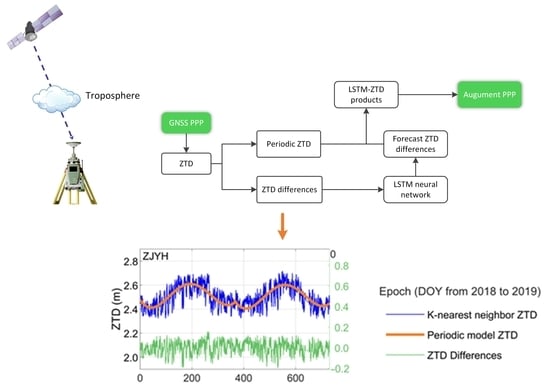
2. Materials and Methods

This study used GNSS observation data from stations of the National Geomatics Center of China (NGCC), their distribution is shown in Figure 2. The parameters and attributes of PPP are listed in Table 1 [24,36]. The zenith hydrostatic delay (ZHD) is derived from the Saastamoinen model, and the zenith wet delay (ZWD) is estimated by static PPP using IGS’s precise orbit and clock products, where the ZTD is obtained by adding the ZWD to the ZHD [37,38].

2.1. Data Preprocessing

Although the PPP-estimated ZTD is sampled with a 30-s interval, the ZTD interval was resampled to a one-hour resolution by retaining only the first ZTD values of each hour. To facilitate data processing, the day of the year (DOY) increases numerically from 1 January 2018, to 31 December 2019. As a result, the accumulated DOY ranges from 1.00 to 730.00, and the corresponding ZTD sample amount is 17,520 (730 × 24).

2.1.1. Outlier Elimination

The ZTD outliers are classified in the stochastic model, and all ZTDs are regarded as equal-weight observation samples [39,40,41]. A fixed-length rolling window was employed to scan the long ZTD series, and if one of the ZTD samples within the window was greater than 3 σ error, it was regarded as a suspicious outlier. Then, the length of the window was expanded to continue iterating until all the ZTD samples met the requirements. Figure 3 shows the ZTD scatter plot before and after the outliers were eliminated. Eliminated outliers and originally observed data gaps result in ZTD time series with discontinuities that form ZTD data gaps.
Figure 3 illustrates that ZTDs are mostly continuous, and only parts of the ZTD data are missing. The statistical results show that the maximum data gap length is no more than 7 days, where most of the ZTD data gap lengths are several hours.

2.1.2. Data Gap Interpolation

In this study, the ZTD data gaps were interpolated with the k-nearest neighbor algorithm (KNN). The KNN interpolates the missing data according to the mean value of the k-nearest samples that neighbor the gap. The principle of the KNN is to obtain ZTD samples based on the nearest Euclidean distance and interpolate the missing data by the inverse distance weighting.
Input parameters for the KNN algorithm are the sampling time and the corresponding ZTD. However, the ZTD series are discontinuous and unevenly spaced. A complete time series with hour-resolution were fed into the KNN algorithm, with the output parameter being interpolated ZTDs. The KNN was implemented with the ‘knn-regression’ module in the scikit-learn package [42]. The k value was set to 720 for model training. The KNN only fills ZTD gaps, hence it retains the original ZTD series.
To validate the proposed data gap interpolation method, we use the periodic model as a reference, which is constructed by Equation (1).
Z T D ( T ) = A 0 + A 1 cos ( 2 π · T ) + B 1 sin ( 2 π · T ) + A 2 cos ( 4 π · T ) + B 2 sin ( 4 π · T )
where T denotes the accumulated DOY from 2018 to 2019, A 0 is the mean value of the ZTD, and ( A 1 , B 1 ) and ( A 2 , B 2 ) are the coefficients of the periodic model, which were calculated with the least squares method.
Figure 4 shows the error comparison of 16-h ZTD interpolated data between the KNN and the periodic model at the CQPS station.
Since the data gap length at each station is not uniform, we take the station CQPS as an example to demonstrate how the KNN fills ZTD gaps. The interpolated ZTDs via the periodic model and the k-nearest neighbor algorithm are smaller than 2 cm from 10:00 to 16:00. However, from 17:00 to 01:00, the errors increase to 6 cm, which implies the accuracies of both models decrease as the gap length increases. Furthermore, after 22:00, the k-nearest neighbor algorithm error begins to decrease from 5.3 to 3.8 cm, whereas the periodic model error remains at about 5.6 cm. We investigated the model accuracy indicators (bias, STD, RMSE, MAE, and R), where the equations for the indicators are as follows: (2)–(5), where N refers to the number of samples, Z T D i p r e is the ZTD value that is output from the models, Z T D i o b s is the original ZTD value as a reference, and Z T D i o b s ¯ and Z T D i p r e ¯ are the mean values of Z T D i o b s and Z T D i p r e , respectively. The periodic model and the KNN-filled ZTD gap within 16 h are shown in Table 2. It demonstrates that the KNN is superior to the periodic model. Therefore, we utilize the KNN to interpolate the ZTD data gaps in this study.
B i a s = 1 N i = 1 N ( Z T D i p r e Z T D i o b s )
S T D = 1 N i = 1 N ( Z T D i p r e Z T D i o b s B i a s ) 2
R M S E = 1 N i = 1 N ( Z T D i p r e Z T D i o b s ) 2
R = i = 1 N ( Z T D i p r e Z T D i p r e ¯ ) ( Z T D i o b s Z T D i o b s ¯ ) i = 1 N ( Z T D i p r e Z T D i p r e ¯ ) 2 i = 1 N ( Z T D i o b s Z T D i o b s ¯ ) 2

2.1.3. GNSS ZTD Testing Accuracy Validation

The global geodetic observing system (GGOS) provided VMF ZTDs with a time resolution of 6 h and a spatial resolution of 1° × 1°. We downloaded VMF3 ZTD products from 1 January 2018 to 31 December 2019 at https://vmf.geo.tuwien.ac.at/trop_products/GRID/1x1/ (accessed on 5 April 2020). The distribution of GNSS stations is sparse. We determine the VMF grid nearest to the GNSS station as a reference, where the criteria are that the longitude and the latitude between approximate GNSS positions and the VMF grid are both less than 0.5° and the altitude difference is less than 100 m. The details are shown in Table 3. We resampled the above preprocessed ZTDs (after eliminating the outliers and filling the ZTD gaps) sampling interval to 6 h by retaining the first ZTD values of every 6 h to validate GNSS ZTD testing accuracy, which were evaluated using Bias, STD, MAE, RMSE, and R. The statistical accuracy indicators are shown in Figure 5. The mean values for Bias, STD, MAE, RMSE and R, which are the testing accuracy indicators, for GNSS ZTDs at GNSS stations are −0.04, 2.44, 1.78, 2.51 and 0.87, respectively.

2.2. LSTM-ZTD Model Construction

2.2.1. ZTD Differences Extraction

After data preprocessing, we obtained the ZTD sequences without outliers and data gaps. ZTD sequences were divided into two parts: training sets (T: 1–510) and testing sets (T: 510–730). The training set was modeled by Equation (1). Figure 6 shows the KNN, the periodic model derived ZTDs, and their differences for the entire dataset. It demonstrates that the periodic model can reflect the annual and semi-annual variation trends. However, their differences vary within 20 cm, without obvious patterns. All seven GNSS stations show negligible bias. The maximum, minimum, and mean RMS values were 6.0, 4.1, and 4.8 cm, respectively.

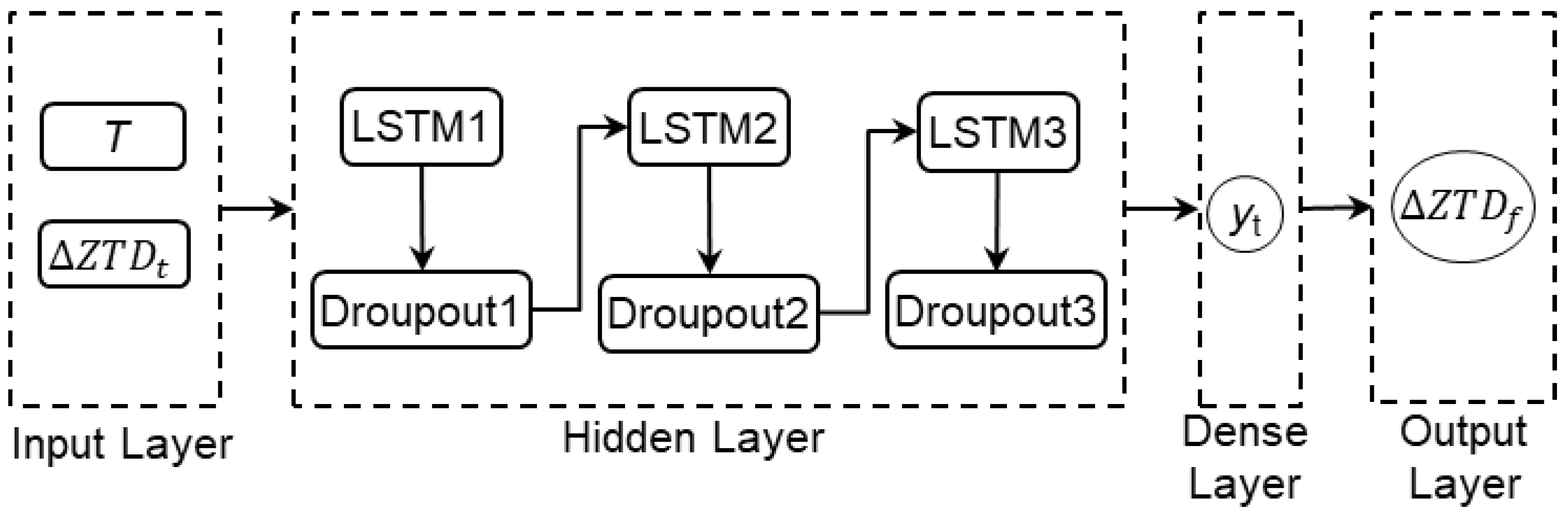
2.2.2. LSTM-ZTD Model Construction

LSTM is one implementation of a recurrent neural network, which can effectively represent time series with long-term patterns [43], and it has been utilized in many fields, including meteorology, network traffic, and air pollution forecasting [44,45,46,47,48]. In the previous section, we extracted differences between the k-nearest neighbor and the periodic model. In this section, we use these differences to train an LSTM neural network. Then, the trained network was used to forecast the ZTD difference during the coming epoch, and finally, the ZTD, by adding the periodic model ZTD. The proposed forecasting model is referred to as LSTM-ZTD in this study.
Figure 7 shows that the LSTM neural network is constructed with multiple layers. The data for the input layer contain ZTD differences ( Δ Z T D t ) between the KNN and the periodic model, with corresponding T. The hidden layer is composed of three LSTM layers (LSTM1, LSTM2, and LSTM3) and their corresponding dropout operation (Dropout1, Dropout2, and Dropout3). These representative features can be extracted as hidden layers from historical input data and connected to a dense layer, which is the fully connected layer that synthesizes features to obtain composite information, y t . The output layer processes y t to output the forecasting results, Δ Z T D f .
A total of 70% (510 days) of the ZTD dataset was used for model training and 30% (220 days) was used for model validation. We chose to use adaptive moment estimation (ADAM) as the optimizer and RMS as the loss function indicator.
Figure 8 demonstrates the network training and validation flow chart. We use the ZTD differences between the KNN and the periodic model over 29 days in a sliding window to predict the next day. One day was treated as a group and the input parameters were divided into 510 groups. The activation function for fully connected layers is tanh, the dropout rate for each LSTM layer is 0.01, the batch size is 40, and the total epochs for training is 10. To obtain the optimum network hyperparameters, the cross-validation strategy was utilized in the training set. More specifically, the training set was divided into 10 equal parts, where 9 parts were used for training, and the remaining part was used for validation [47,49,50]. It takes 6.64 h to train the model on a supercomputing system in the Supercomputing Center of Wuhan University. The supercomputing system is equipped with 2580.175 MHz, 20 cores CPU, and 128 G RAM.

3. Results and Analysis

Firstly, ZTDs from T 510 to 730 are used to validate the LSTM-ZTD forecasting model. Secondly, the forecasted ZTDs are used for tropospheric delay correction for PPP.

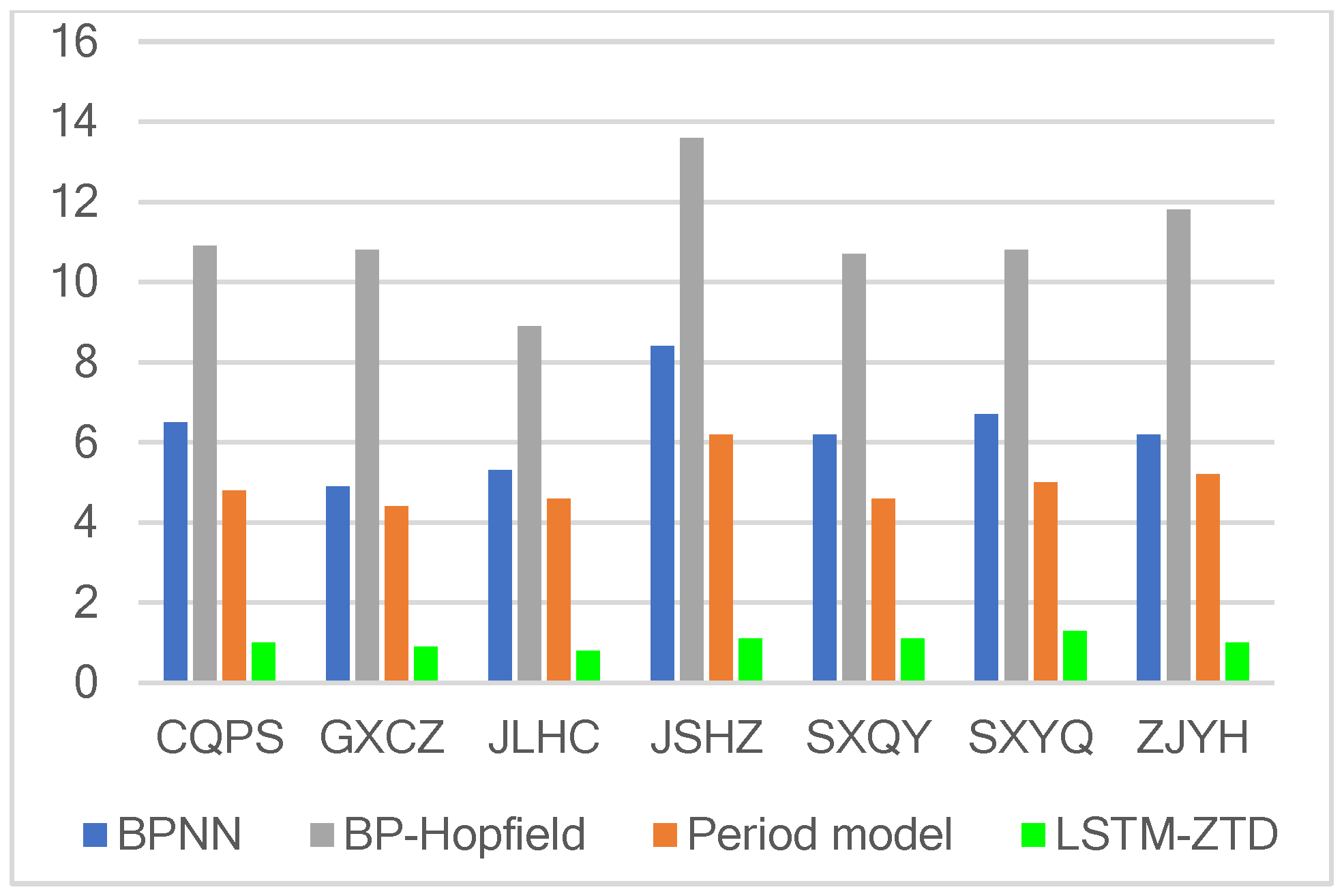
3.1. Validation from ZTD Models Perspective

Figure 9 shows the ZTD series comparison for 220-day forecasts using different models (i.e., the BPNN, the BP–Hopfield, the KNN, and the LSTM-ZTD model). Among these models, the KNN derived ZTD series was selected as the reference. The LSTM-ZTD results are close to those of the KNN derived ZTD series, indicating that the proposed model can forecast complex ZTD changes. The BPNN model and the BP–Hopfield model products can only just reflect the approximate trend.
Figure 10 shows the RMSE comparison among the BPNN, BP–Hopfield, period model, and LSTM-ZTD errors. It demonstrates that the LSTM-ZTD model is superior to the other models, by more than about 1 cm. The mean RMSE error of the LSTM-ZTD model for seven stations is 1.0 cm.

3.2. Validation from PPP Perspective

The tropospheric wet delay is generally estimated as an unknown parameter in PPP. The tropospheric delay can be expressed by the following model:
T r = T r 0 + M w ( E ) · Δ T r z , w
T r 0 = M h ( E ) · T r z , h + M w ( E ) · T r z , w 0
where T r 0 is the modeled tropospheric delay, M h ( E ) and M w ( E ) are the projection functions of ZHD and ZWD, respectively, Δ T r z , w is the unmodelled ZWD, T r z , h is the modeled ZHD, and T r z , w 0 is the modelled ZWD [22,49,51]. M h ( E ) and M w ( E ) are the NMF (Niell 1996), which do not require any meteorological data, and E is the elevation angle [24,50]. More details of the corresponding processing solutions are shown in Table 1 and Table 4.
Tropospheric augmentation information can reduce PPP convergence time [22,52,53]. Mendez Astudillo et al., (2018) found that the convergence time of PPP is affected by seasonal variations [49], and the forecasted ZTD series from T 510 to 730 involve three seasons, namely summer, autumn, and winter. The positioning experiment was carried out using observational data and ZTD series were forecasted for three GNSS stations (JSHZ, SXQY, SXYQ) in the summer (T 514, May 29), autumn (T 608, August 31), and winter (T 693, November 24).
We investigated the convergence time to verify the feasibility of LSTM-ZTD corrected PPP (L-PPP), as well as GPT2 ZTD corrected PPP (G-PPP). Unlike conventional ionospheric-free combined PPP, LSTM-ZTD corrected PPP and GPT2 ZTD corrected PPP add a virtual observation for ZTD and its corresponding constraint on the observation equation [21]. In this study, we define the convergence time as a reverse search from the last epoch to the first epoch, until the error during one epoch in one of the E, N, or U directions exceeds 10 cm.
Table 5 shows the convergence times of LSTM-ZTD corrected PPP compared with GPT2 ZTD corrected PPP and conventional PPP. It shows that the LSTM-ZTD corrected PPP convergence time is shorter than GPT2 ZTD corrected PPP and conventional PPP. The convergence time of GPT2 ZTD corrected PPP was reduced by 4.8%, and the convergence time of LSTM-ZTD corrected PPP was reduced by 13.9% in the summer. Those two solutions were reduced by 13.7% and 22.6% in the autumn season and reduced by 13.8% and 30.7% in the winter season, respectively, compared to conventional PPP.

4. Conclusions

In this study, we proposed an LSTM-ZTD forecasting model. GNSS observations provided by the NGCC during 2018–2019 were used to establish and validate the proposed model. Firstly, the ZTDs were estimated using static PPP and the outliers were eliminated. Secondly, the k-nearest neighbor algorithm was applied to interpolate ZTD data gaps. Numerical results show that the KNN is superior to the periodical model in interpolating ZTD data gaps. Thirdly, ZTD differences between the k-nearest neighbor and periodic model were used to train an LSTM neural network. LSTM forecasted ZTD differences and periodic model derived ZTDs were combined to recover the forecasted ZTDs. Finally, a static PPP experiment was performed to validate and develop the LSTM-ZTD model.
Conclusions are summarized as follows: (1) The ZTD forecast error of the proposed LSTM model is about 1.0 cm, superior to that of the Hopfield (8.4 cm), BPNN (6.3 cm), and BP–Hopfield (11.1 cm), and periodic model (5.0 cm); (2) The GPT2 ZTD corrected PPP convergence time was reduced by 4.8, 13.7, and 13.8% in the summer, autumn, and winter seasons, respectively. The LSTM-ZTD corrected PPP convergence time was reduced by 13.9, 22.6, and 30.7% in the summer, autumn, and winter seasons, respectively, which are superior to conventional PPP.

Author Contributions

Conceptualization H.Z. and C.X.; investigation H.Z. and Y.Y.; data curation H.Z.; methodology Y.Y. and H.Z.; program H.Z. and M.H.; validation Y.Y. and C.X.; design of the study H.Z. and X.S.; writing—original draft preparation H.Z. and D.C.; writing—review and editing M.H. and W.P.; formal analysis M.H. and H.Z. All authors have read and agreed to the published version of the manuscript.

Funding

This research was funded by the National Natural Science Foundation of China (Nos. 41874033, 41721003, and 42004019). The key research and development plan of Guilin, China (2020010315), and the Guangxi Science and Technology Plan Project Technology Innovation Guidance Special (AC20238007). The Center of National Railway Intelligent Transportation System Engineering and Technology (Contract No. 2021YJ194), China Academy of Railway Sciences.

Data Availability Statement

The GNSS station observation dataset can be obtained from the National Geomatics Center of China (NGCC). Due to a classification level of ‘secret’, the data are not publicly available on the network and cannot be accessed via hyperlinks. However, the results are available from this email (johnhuan@whu.edu.cn). The temperature and pressure data can be obtained from the ECMWF Climate Change Service at https://cds.climate.copernicus.eu (accessed on 20 May 2020).

Acknowledgments

The authors would like to thank the National Geomatics Center of China (NGCC) for providing observational data for GNSS stations for calculating tropospheric delay and performing positioning experiments. Thanks to the ECMWF Climate Change Service for providing the temperature and pressure data. The numerical calculations in this paper have been performed on the supercomputing system in the Supercomputing Center of Wuhan University.

Conflicts of Interest

The authors declare no conflict of interest.

Abbreviations

ZTDZenith tropospheric delay
ZHDZenith hydrostatic delay
ZWDZenith wet delay
GNSSGlobal navigation satellite system
PPPPrecise point position
RTKReal-Time Kinematic positioning
NGCCThe National Geomatics Center of China
LSTMLong short-term memory
ECMWFThe European Centre for Medium-Range Weather Forecasts
BPNNBack Propagation Neural Network
RMSERoot-mean-square error
STDStandard deviation
IGSInternational GNSS service
RTSReal-time service
EGNOSEuropean Geostationary Navigation Overlay Service
UNBUniversity of New Brunswick model
GPTThe global temperature and pressure
ICAIndependent component analysis
PCAPrincipal component analysis
DOYDay of year
HODHour of day
RAMRandom access memory
L-PPPLSTM-ZTD constrained PPP
C-PPPConventional ionospheric-free combined PPP
TAccumulated DOY from 2018 to 2019

References

  1. Blewitt, G. Carrier phase ambiguity resolution for the Global Positioning System applied to geodetic baselines up to 2000 km. J. Geophys. Res. Solid Earth 1989, 94, 10187–10203. [Google Scholar] [CrossRef] [Green Version]
  2. Malys, S.; Jensen, P.A. Geodetic Point Positioning with GPS Carrier Beat Phase Data from the CASA UNO Experiment. Geophys. Res. Lett. 1990, 17, 651–654. [Google Scholar] [CrossRef]
  3. Zumberge, J.; Heflin, M.; Jefferson, D.; Watkins, M.; Webb, F. Precise point positioning for the efficient and robust analysis of GPS data from large networks. J. Geophys. Res. Solid Earth 1997, 102, 5005–5017. [Google Scholar] [CrossRef] [Green Version]
  4. Kouba, J. Implementation and testing of the gridded Vienna Mapping Function 1 (VMF1). J. Geod. 2008, 82, 193–205. [Google Scholar] [CrossRef]
  5. Tao, Y.; Liu, C.; Liu, C.; Zhao, X.; Hu, H. Empirical Wavelet Transform Method for GNSS Coordinate Series Denoising. J. Geovis. Spatial Anal. 2021, 5, 9. [Google Scholar] [CrossRef]
  6. Bevis, M.; Businger, S.; Herring, T.A.; Rocken, C.; Anthes, R.A.; Ware, R.H. GPS meteorology: Remote sensing of atmospheric water vapor using the Global Positioning System. J. Geophys. Res. Atmos. 1992, 97, 15787–15801. [Google Scholar] [CrossRef]
  7. Kos, T.; Botincan, M.; Markezic, I. Estimation of tropospheric delay models compliance. In Proceedings of the 2008 50th International Symposium ELMAR, Borik Zadar, Croatia, 10–12 September 2022; IEEE: Piscataway, NJ, USA, 2008; Volume 2, pp. 381–384. [Google Scholar]
  8. Saastamoinen, J. Contributions to the theory of atmospheric refraction. Bull. Géodésique 1973, 107, 13–34. [Google Scholar] [CrossRef]
  9. Black, H.D. An easily implemented algorithm for the tropospheric range correction. J. Geophys. Res. Solid Earth 1978, 83, 1825–1828. [Google Scholar] [CrossRef]
  10. Hopfield, H. Two-quartic tropospheric refractivity profile for correcting satellite data. J. Geophys. Res. 1969, 74, 4487–4499. [Google Scholar] [CrossRef]
  11. Penna, N.; Dodson, A.; Chen, W. Assessment of EGNOS tropospheric correction model. J. Navig. 2001, 54, 37–55. [Google Scholar] [CrossRef]
  12. Collins, J.P.; Langley, R.B. A Tropospheric Delay Model for the User of the Wide Area Augmentation System; Department of Geodesy and Geomatics Engineering, University of New Brunswick: Fredericton, NB, Canada, 1997. [Google Scholar]
  13. Leandro, R.; Santos, M.; Langley, R. “UNB Neutral Atmosphere Models: Development and Performance”. In Proceedings of the 2006 National Technical Meeting of The Institute of Navigation, Monterey, CA, USA, 18–20 January 2006; pp. 564–573. [Google Scholar]
  14. Böhm, J.; Möller, G.; Schindelegger, M.; Pain, G.; Weber, R. Development of an improved empirical model for slant delays in the troposphere (GPT2w). GPS Solut. 2015, 19, 433–441. [Google Scholar] [CrossRef] [Green Version]
  15. Bock, O.; Willis, P.; Wang, J.; Mears, C. A high-quality, homogenized, global, long-term (1993–2008) DORIS precipitable water data set for climate monitoring and model verification. J. Geophys. Res. Atmos. 2014, 119, 7209–7230. [Google Scholar] [CrossRef]
  16. Alshawaf, F.; Zus, F.; Balidakis, K.; Deng, Z.; Hoseini, M.; Dick, G.; Wickert, J. On the statistical significance of climatic trends estimated from GPS tropospheric time series. J. Geophys. Res. Atmos. 2018, 123, 10–967. [Google Scholar] [CrossRef] [Green Version]
  17. De Haan, S. Assimilation of GNSS ZTD and radar radial velocity for the benefit of very short-range regional weather forecasts. Q. J. R. Meteorol. Soc. 2013, 139, 2097–2107. [Google Scholar] [CrossRef]
  18. Nowel, K. Specification of deformation congruence models using combinatorial iterative DIA testing procedure. J. Geod. 2020, 94, 1–23. [Google Scholar] [CrossRef]
  19. Yang, L.; Shen, Y.; Li, B.; Rizos, C. Simplified algebraic estimation for the quality control of DIA estimator. J. Geod. 2021, 95, 1–15. [Google Scholar] [CrossRef]
  20. Hadas, T.; Kaplon, J.; Bosy, J.; Sierny, J.; Wilgan, K. Near-real-time regional troposphere models for the GNSS precise point positioning technique. Meas. Sci. Technol. 2013, 24, 055003. [Google Scholar] [CrossRef]
  21. Shi, J.; Xu, C.; Guo, J.; Gao, Y. Local troposphere augmentation for real-time precise point positioning. Earth Planets Space 2014, 66, 1–13. [Google Scholar] [CrossRef] [Green Version]
  22. Yao, Y.; Peng, W.; Xu, C.; Cheng, S. Enhancing real-time precise point positioning with zenith troposphere delay products and the determination of corresponding tropospheric stochastic models. Geophys. Suppl. Mon. Not. R. Astron. Soc. 2016, 208, 1217–1230. [Google Scholar] [CrossRef]
  23. De Oliveira, P.; Morel, L.; Fund, F.; Legros, R.; Monico, J.; Durand, S.; Durand, F. Modeling tropospheric wet delays with dense and sparse network configurations for PPP-RTK. GPS Solut. 2017, 21, 237–250. [Google Scholar] [CrossRef]
  24. Zhang, H.; Yuan, Y.; Li, W. Real-time wide-area precise tropospheric corrections (WAPTCs) jointly using GNSS and NWP forecasts for China. J. Geod. 2022, 96, 1–18. [Google Scholar] [CrossRef]
  25. Chen, W.; Gao, C.; Pan, S. Assessment of GPT2 empirical troposphere model and application analysis in precise point positioning. In Proceedings of the China Satellite Navigation Conference (CSNC) 2014 Proceedings, Berlin, Germany, 26 April 2014; Volume II. [Google Scholar]
  26. Song, C.; Hao, J.; Zhang, H. A Method to Accelerate PPP Re-Convergence with Prior Troposphere Delay Constraint. J. Geom. Sci. Technol. 2015, 32, 441–444. [Google Scholar]
  27. Jia, S.; Min, L.; Qile, Z.; Zhiqiang, D. A Real Time Regional Zenith Troposphere Delay Model and Its Application in PPP. Bull. Surv. Mapp. 2018, 4, 1. [Google Scholar]
  28. Nikolaidou, T.; Nievinski, F.; Balidakis, K.; Schuh, H.; Santos, M. PPP without troposphere estimation: Impact assessment of regional versus global numerical weather models and delay parametrization. In Proceedings of the International Symposium on Advancing Geodesy in a Changing World, Kobe, Japan, 30 July–4 August 2018; Springer: Cham, Germany, 2018; pp. 107–118. [Google Scholar]
  29. Pikridas, C.; Katsougiannopoulos, S.; Ifadis, I. Predicting Zenith Tropospheric Delay using the Artificial Neural Network technique. Application to selected EPN stations. J. Nat. Cancer Inst. 2010, 88, 1803–1805. [Google Scholar]
  30. Wang, Y.; Zhang, L.; Yang, J. Prediction of zenith tropospheric delay based on BP neural network. In Advances in Computer Science and Education; Springer: Berlin/Heidelberg, Germany, 2012; pp. 459–465. [Google Scholar]
  31. Zhang, Q.; Li, F.; Zhang, S.; Li, W. Modeling and forecasting the GPS zenith troposphere delay in West Antarctica based on different blind source separation methods and deep learning. Sensors 2020, 20, 2343. [Google Scholar] [CrossRef] [Green Version]
  32. Ding, M.; Hu, W.; Jin, X.; Yu, L. A new ZTD model based on permanent ground-based GNSS-ZTD data. Surv. Rev. 2015, 48, 385–391. [Google Scholar] [CrossRef]
  33. Xiao, G.; Ou, J.; Liu, G.; Zhang, H. Construction of a regional precise tropospheric delay model based on improved BP neural network. Chin. J. Geophys. 2018, 61, 3139–3148. [Google Scholar]
  34. Yang, Y.; Xu, T.; Ren, L. A new regional tropospheric delay correction model based on BP neural network. In Proceedings of the 2017 Forum on Cooperative Positioning and Service (CPGPS), Harbin, China, 19–21 May 2017; IEEE: Piscataway, NJ, USA, 2017; pp. 96–100. [Google Scholar]
  35. Zheng, D.; Hu, W.; Wang, J.; Zhu, M. Research on regional zenith tropospheric delay based on neural network technology. Surv. Rev. 2015, 47, 286–295. [Google Scholar] [CrossRef]
  36. Yao, Y.; Xu, X.; Xu, C.; Peng, W.; Wan, Y. GGOS tropospheric delay forecast product performance evaluation and its application in real-time PPP. J. Atmosph. Solar-Terr. Phys. 2018, 175, 1–17. [Google Scholar] [CrossRef]
  37. Boehm, J.; Niell, A.; Tregoning, P.; Schuh, H. Global Mapping Function (GMF): A new empirical mapping function based on numerical weather model data. Geophys. Res. Lett. 2006, 33, L07304. [Google Scholar] [CrossRef] [Green Version]
  38. Gao, Y.; Chen, K. Performance analysis of precise point positioning using real-time orbit and clock products. J. Glob. Position. Syst. 2004, 3, 95–100. [Google Scholar] [CrossRef]
  39. Baarda, W. Statistical Concepts in Geodesy; Netherlands Geodetic Commission: Amersfoort, The Netherlands, 1967; Volume 2, pp. 1–74. [Google Scholar]
  40. Li, B.; Zhao, K.; Sandoval, E.B. A UWB-Based Indoor Positioning System Employing Neural Networks. J. Geovis. Spat. Anal. 2020, 4, 18. [Google Scholar] [CrossRef]
  41. Baarda, W. A Testing Procedure for Use in Geodetic Networks; Netherlands Geodetic Commission: Amersfoort, The Netherlands, 1968; Volume 2, pp. 1–97. [Google Scholar]
  42. Pedregosa, F.; Varoquaux, G.; Gramfort, A.; Michel, V.; Thirion, B.; Grisel, O.; Duchesnay, E. Scikit-learn: Machine Learning in Python. JMLR 2011, 12, 2825–2830. [Google Scholar]
  43. Hochreiter, S.; Schmidhuber, J. Long short-term memory. Neural Comput. 1997, 9, 1735–1780. [Google Scholar] [CrossRef] [PubMed]
  44. Hu, Y.L.; Chen, L. A nonlinear hybrid wind speed forecasting model using LSTM network, hysteretic ELM and Differential Evolution algorithm. Energy Convers. Manag. 2018, 173, 123–142. [Google Scholar] [CrossRef]
  45. Qing, X.; Niu, Y. Hourly day-ahead solar irradiance prediction using weather forecasts by LSTM. Energy 2018, 148, 461–468. [Google Scholar] [CrossRef]
  46. Zhao, Z.; Chen, W.; Wu, X.; Chen, P.C.; Liu, J. LSTM network: A deep learning approach for short-term traffic forecast. IET Intell. Transp. Syst. 2017, 11, 68–75. [Google Scholar] [CrossRef] [Green Version]
  47. Huang, B.; Ji, Z.; Zhai, R.; Xiao, C.; Yang, F.; Yang, B.; Wang, Y. Clock bias prediction algorithm for navigation satellites based on a supervised learning long short-term memory neural network. GPS Solut. 2021, 25, 1–16. [Google Scholar] [CrossRef]
  48. Liu, L.; Zou, S.; Yao, Y.; Wang, Z. Forecasting global ionospheric TEC using deep learning approach. Space Weather 2020, 18, e2020SW002501. [Google Scholar] [CrossRef]
  49. Mendez Astudillo, J.; Lau, L.; Tang, Y.T.; Moore, T. Analysing the zenith tropospheric delay estimates in on-line precise point positioning (PPP) services and PPP software packages. Sensors 2018, 18, 580. [Google Scholar] [CrossRef] [Green Version]
  50. Zhang, H.; Yao, Y.; Xu, C.; Xu, W.; Shi, J. Transformer-Based Global Zenith Tropospheric Delay Forecasting Model. Remote Sens. 2022, 14, 3335. [Google Scholar] [CrossRef]
  51. Wilgan, K.; Hurter, F.; Geiger, A.; Rohm, W.; Bosy, J. Tropospheric refractivity and zenith path delays from least-squares collocation of meteorological and GNSS data. J. Geod. 2017, 91, 117–134. [Google Scholar] [CrossRef] [Green Version]
  52. Niell, A.E. Global mapping functions for the atmosphere delay at radio wavelengths. J. Geophys. Res. Solid Earth 1996, 101, 3227–3246. [Google Scholar] [CrossRef]
  53. Vaclavovic, P.; Dousa, J.; Elias, M.; Kostelecky, J. Using external tropospheric corrections to improve GNSS positioning of hot-air balloon. GPS Solut. 2017, 21, 1479–1489. [Google Scholar] [CrossRef]
Figure 1. Main procedures flow chart to establish the LSTM-ZTD forecast model.
Remotesensing 14 05921 g001
Figure 2. Distribution of GNSS stations in this study.
Remotesensing 14 05921 g002
Figure 3. ZTD time series of seven GNSS stations before (left) and after (right) the outliers were eliminated. A red box marks obvious outliers in the left panel. N = 730, representing two years, collected from 1 January 2018 to 31 December 2019.
Remotesensing 14 05921 g003
Figure 4. The KNN and periodic model interpolated ZTD error comparison from 10:00 on 3 December 2018 to 1:00 on December 4 at the CQPS station.
Remotesensing 14 05921 g004
Figure 5. Testing the accuracy between GNSS ZTD and VMF ZTD (cm).
Remotesensing 14 05921 g005
Figure 6. Comparison between the KNN and the periodic model. N = 730, the blue and orange curves show the KNN and periodic model derived ZTDs, respectively. The green curve shows ZTD series differences between the two models.
Remotesensing 14 05921 g006
Figure 7. LSTM neural network structure designed in this study.
Remotesensing 14 05921 g007
Figure 8. Network training and validation flow chart. The red box shows the input parameter, which consists of T and the ZTD differences ( Δ Z T D t ) between the KNN and the periodic model. The blue box expresses the training sets, the orange box shows the validation sets, and the red circle represents the original differences between KNN and the periodic model. The green box shows the output forecasting results, Δ Z T D f .
Remotesensing 14 05921 g008
Figure 9. The ZTD series and their errors. Comparisons among different models. Each panel represents a station, where the blue, purple, cyan, and red curves show the BPNN, BP–Hopfield, KNN, and LSTM-ZTD models, respectively. The dark green, orange, and light green curves show the errors in the BP–Hopfield, BPNN, and LSTM-ZTD models, respectively.
Remotesensing 14 05921 g009
Figure 10. RMS error (cm) comparison of different forecasting models.
Remotesensing 14 05921 g010
Table 1. Strategies used in the PPP program.
ItemsStrategies
ObservationsGPS/GLONASS raw pseudo range and phase observables
Frequency selectionL1 & L2
Orbit and clockIGS final products
Sampling rate30 s
Combination modeIF combinations
Ambiguity FixedFloat solutions (random walk process 10−4 mm/ h )
Weight for observationsElevation-dependent weight
Phase windup effectCorrected
Station coordinatesFixed
Station displacementSolid Earth tides, ocean tides, and pole tide displacements
Satellite/receiver PCO/PCVIGS14_2156.atx
DCBCODE P1-C1
Elevation angle
Sampling rate30 s
ZHDSaastamoinen
Mapping functionNMF
Orbit and clock errorsGBM final orbit and clock
Parameter estimatorKalman filter (smooth)
Table 2. Accuracy comparison between the KNN and the periodical model for data gap interpolation.
ModelBias (cm)STD (cm)RMS (cm)RMAE (cm)
Periodic model ZTD2.991.963.570.782.99
KNN ZTD2.771.523.160.862.77
Table 3. Spatial information of approximate GNSS station positions and the VMF grid.
GNSS Stations APPROX POSITIONVMF Grid
StationsLon (°)Lat (°)Lon (°)Lat (°)
CQPS108.22229.359108.529.5
GXCZ107.32222.391107.522.5
JLHC131.10443.223131.543.5
JSHZ118.91333.307118.533.5
SXQY112.33536.509112.536.5
SXYQ111.66035.277111.535.5
ZJYH119.68928.266119.528.5
Table 4. Processing solutions of PPP.
Conventional PPPGPT2-ZTD Corrected PPPLSTM-ZTD Corrected PPP
Troposphere ZWDEstimation
(Random walk process
10 mm/ h )
GPT2-ZTD and estimation
(Random walk process
10 mm/ h )
LSTM-ZTD and estimation
(Random walk process
10 mm/ h )
Initial ZTDSaastamoinenThe first of GPT2-ZTDThe first of LSTM-ZTD
Table 5. PPP convergence time statistics of conventional ZTD corrected PPP (T-PPP) and LSTM-ZTD constrained PPP (L-PPP) (min).
StationsSummer (T 514)Autumn (T 608)Winter (T 693)
C-PPPG-PPPL-PPPC-PPPG-PPPL-PPPC-PPPG-PPPL-PPP
JSHZ2625.523.522.5212117128
SXQY23.52321.515.512.512.510.5109.5
SXYQ24.5252215.51514.5201610.5
GXCZ262418.51612917.515.513.5
CQPS23.52222.519.51613.521.518.514
JLHC26.521.521.520.51814222116.5
ZJYH161713.514.512.511.518.516.516
Average23.722.620.417.715.313.718.115.612.6
The C-PPP denotes conventional PPP, G-PPP denotes GPT2 ZTD corrected PPP and L-PPP denotes LSTM-ZTD corrected PPP.
Publisher’s Note: MDPI stays neutral with regard to jurisdictional claims in published maps and institutional affiliations.

