
Lidar- and V2X-Based Cooperative Localization Technique for Autonomous Driving in a GNSS-Denied Environment


Abstract
: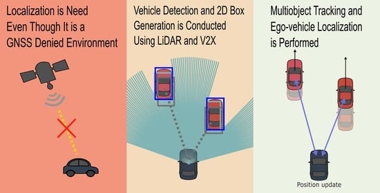
1. Introduction
2. Sensor Fusion and Localization
2.1. Overview
2.2. Data Processing
2.3. Sensor Fusion for Surrounding Vehicles
2.4. Localization for the Ego-vehicle
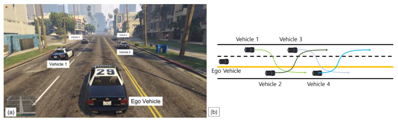
3. Experiments
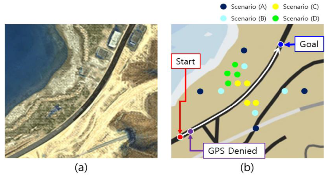
3.1. Experimental Environment Configuration
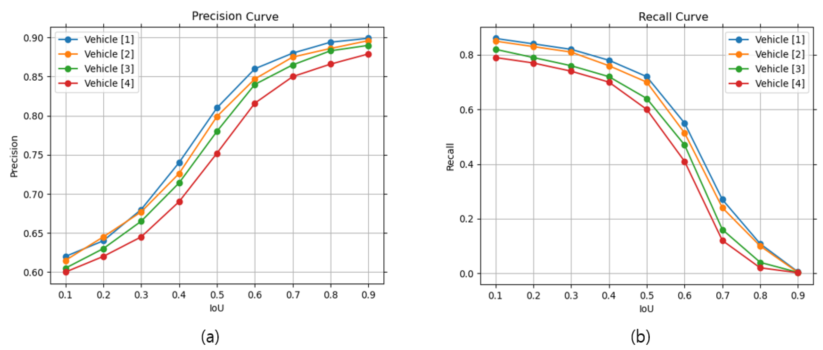
3.2. Sensor Fusion and Multiobject Tracking Result of Surrounding Vehicles
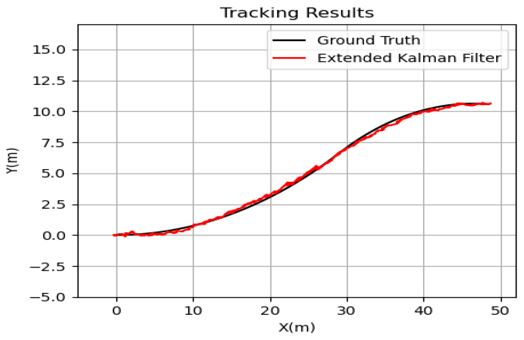
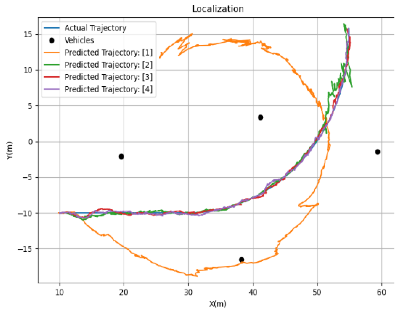
3.3. Localization Results for the Ego-vehicle
4. Conclusions
Author Contributions
Funding
Conflicts of Interest
References
- Koopman, P.; Wagner, M. Autonomous vehicle safety: An interdisciplinary challenge. IEEE Intell. Transp. Syst. Mag. 2017, 9, 90–96. [Google Scholar] [CrossRef]
- Van Brummelen, J.; O’Brien, M.; Gruyer, D.; Najjaran, H. Autonomous vehicle perception: The technology of today and tomorrow. Transp. Res. Part C Emerg. Technol. 2018, 89, 384–406. [Google Scholar] [CrossRef]
- Varghese, J.Z.; Boone, R.G. Overview of autonomous vehicle sensors and systems. In Proceedings of the 2015 International Conference on Operations Excellence and Service Engineering, Orlando, FL, USA, 10–11 September 2015; pp. 178–191. [Google Scholar]
- Kaplan, E.D.; Hegarty, C. Understanding GPS/GNSS: Principles and Applications; Artech House: Norwood, MA, USA, 2017. [Google Scholar]
- Nazaruddin, Y.Y.; Maani, F.A.; Muten, E.R.; Sanjaya, P.W.; Tjahjono, G.; Oktavianus, J.A. An Approach for the Localization Method of Autonomous Vehicles in the Event of Missing GNSS Information. In Proceedings of the 2021 60th Annual Conference of the Society of Instrument and Control Engineers of Japan (SICE), Tokyo, Japan, 8–10 September 2021; pp. 881–886. [Google Scholar]
- Aftatah, M.; Lahrech, A.; Abounada, A.; Soulhi, A. GPS/INS/Odometer data fusion for land vehicle localization in GPS denied environment. Mod. Appl. Sci. 2016, 11, 62. [Google Scholar] [CrossRef]
- Magree, D.; Johnson, E.N. Combined Laser and Vision aided Inertial Navigation for an Indoor Unmanned Aerial Vehicle. In Proceedings of the 2014 American Control Conference, Portland, OR, USA, 4–6 June 2014; pp. 1900–1905. [Google Scholar]
- Conte, G.; Doherty, P. An Integrated UAV Navigation System Based on Aerial Image Matching. In Proceedings of the 2008 IEEE Aerospace Conference, Big Sky, MT, USA, 1–8 March 2008; pp. 1–10. [Google Scholar]
- Gu, D.Y.; Zhu, C.F.; Guo, J.; Li, S.X.; Chang, H.X. Vision-aided UAV navigation using GIS data. In Proceedings of 2010 IEEE International Conference on Vehicular Electronics and Safety, Qingdao, China, 15–17 July 2010; pp. 78–82. [Google Scholar]
- Abboud, K.; Omar, H.A.; Zhuang, W. Interworking of DSRC and Cellular Network Technologies for V2X Communications: A Survey. IEEE Trans. Veh. Technol. 2016, 65, 9457–9470. [Google Scholar] [CrossRef]
- Kim, J.S.; Choi, W.Y.; Jeong, Y.W.; Chung, C.C. Vehicle Localization Using Radar Calibration with Disconnected GPS. In Proceedings of the 2021 21st International Conference on Control, Automation and Systems (ICCAS), Jeju, Republic of Korea, 12–15 October 2021; pp. 1371–1376. [Google Scholar]
- Ma, S.; Wen, F.; Zhao, X.; Wang, Z.M.; Yang, D. An efficient V2X based vehicle localization using single RSU and single receiver. IEEE Access 2019, 7, 46114–46121. [Google Scholar] [CrossRef]
- Perea-Strom, D.; Morell, A.; Toledo, J.; Acosta, L. GNSS integration in the localization system of an autonomous vehicle based on Particle Weighting. IEEE Sens. J. 2020, 20, 3314–3323. [Google Scholar] [CrossRef]
- Asvadi, A.; Girao, P.; Peixoto, P.; Nunes, U. 3D object tracking using RGB and LIDAR data. In Proceedings of the 2016 IEEE 19th International Conference on Intelligent Transportation Systems (ITSC), Rio de Janeiro, Brazil, 1–4 November 2016; pp. 1255–1260. [Google Scholar]
- Qi, Y.; Yao, H.; Sun, X.; Sun, X.; Zhang, Y.; Huang, Q. Structure-aware multi-object discovery for weakly supervised tracking. In Proceedings of the 2014 IEEE International Conference on Image Processing (ICIP), Paris, France, 27–30 October 2014; pp. 466–470. [Google Scholar]
- Qi, Y.; Zhang, S.; Qin, L.; Yao, H.; Huang, Q.; Lim, J.; Yang, M.H. Hedged deep tracking. In Proceedings of the IEEE Conference on Computer Vision and Pattern Recognition, Las Vegas, NV, USA, 27–30 June 2016; pp. 4303–4311. [Google Scholar]
- Voigtlaender, P.; Luiten, J.; Torr, P.H.; Leibe, B. Siam r-cnn: Visual tracking by re-detection. In Proceedings of the IEEE/CVF Conference on Computer Vision and Pattern Recognition, Seattle, WA, USA, 13–19 June 2020; pp. 6578–6588. [Google Scholar]
- Fujii, S.; Fujita, A.; Umedu, T.; Kaneda, S.; Yamaguchi, H.; Higashino, T.; Takai, M. Cooperative vehicle positioning via V2V communications and onboard sensors. In Proceedings of the 2011 IEEE Vehicular Technology Conference (VTC Fall), San Francisco, CA, USA, 5–8 September 2011; pp. 1–5. [Google Scholar]
- Li, Y.; Ibanez-Guzman, J. Lidar for autonomous driving: The principles, challenges, and trends for automotive lidar and perception systems. IEEE Signal Process. Mag. 2020, 37, 50–61. [Google Scholar] [CrossRef]
- Zhang, X.; Xu, W.; Dong, C.; Dolan, J.M. Efficient L-shape fitting for vehicle detection using laser scanners. In Proceedings of the 2017 IEEE Intelligent Vehicles Symposium (IV), Los Angeles, CA, USA, 11–14 June 2017; pp. 54–59. [Google Scholar]
- Kim, J.K.; Kim, J.W.; Kim, J.H.; Jung, T.H.; Park, Y.J.; Ko, Y.H.; Jung, S. Experimental studies of autonomous driving of a vehicle on the road using LiDAR and DGPS. In Proceedings of the 2015 15th International Conference on Control, Automation and Systems (ICCAS), Busan, Republic of Korea, 13–16 October 2015; pp. 1366–1369. [Google Scholar]
- Wu, H.; Siegel, M.; Stiefelhagen, R.; Yang, J. Sensor fusion using Dempster-Shafer theory [for context-aware HCI]. IMTC/2002. In Proceedings of the 19th IEEE Instrumentation and Measurement Technology Conference (IEEE Cat. No.00CH37276), Anchorage, AK, USA, 21–23 May 2002; Volume 1, pp. 7–12. [Google Scholar]
- Snoek, C.G.M.; Worring, M.; Smeulders, A.W.M. Early versus late fusion in semantic video analysis. In Proceedings of the 13th Annual ACM International Conference on Multimedia, Singapore, 6–11 November 2005; pp. 399–402. [Google Scholar]
- Wojke, N.; Bewley, A.; Paulus, D. Simple online and realtime tracking with a deep association metric. In Proceedings of the 2017 IEEE International Conference on Image Processing (ICIP), Beijing, China, 17–20 September 2017; pp. 3645–3649. [Google Scholar]
- Mauri, A.; Khemmar, R.; Decoux, B.; Ragot, N.; Rossi, R.; Trabelsi, R.; Boutteau, R.; Ertaud, J.Y.; Savatier, X. Deep Learning for Real-Time 3D Multi-Object Detection, Localisation, and Tracking: Application to Smart Mobility. Sensors 2020, 20, 532. [Google Scholar] [CrossRef] [PubMed] [Green Version]
- Zhou, D.; Fang, J.; Song, X.; Guan, C.; Yin, J.; Dai, Y.; Yang, R. Iou loss for 2d/3d object detection. In Proceedings of the 2019 International Conference on 3D Vision (3DV), Québec, QC, Canada, 16–19 September 2019; pp. 85–94. [Google Scholar]
- Kramer, B.; MacKinnon, A. Localization: Theory and experiment. Rep. Prog. Phys. 1993, 56, 1469. [Google Scholar] [CrossRef]
- Kaune, R. Accuracy studies for TDOA and TOA localization. In Proceedings of the 2012 15th International Conference on Information Fusion, Singapore, 9–12 July 2012; pp. 408–415. [Google Scholar]
- Xue, W.; Qiu, W.; Hua, X.; Yu, K. Improved Wi-Fi RSSI measurement for indoor localization. IEEE Sens. J. 2017, 17, 2224–2230. [Google Scholar] [CrossRef]
- Wann, C.D.; Yeh, Y.J.; Hsueh, C.S. Hybrid TDOA/AOA indoor positioning and tracking using extended Kalman filters. In Proceedings of the 2006 IEEE 63rd Vehicular Technology Conference, Melbourne, Australia, 7–10 May 2006; pp. 1058–1062. [Google Scholar]
- Bailey, T.; Nieto, J.; Guivant, J.; Stevens, M.; Nebot, E. Consistency of the EKF-SLAM algorithm. In Proceedings of the 2006 IEEE/RSJ International Conference on Intelligent Robots and Systems, Beijing, China, 9–15 October 2006; pp. 3562–3568. [Google Scholar]
- Wen, W.; Hsu, L.T.; Zhang, G. Performance analysis of NDT-based graph SLAM for autonomous vehicle in diverse typical driving scenarios of Hong Kong. Sensors 2018, 18, 3928. [Google Scholar] [CrossRef] [PubMed] [Green Version]
- Mur-Artal, R.; Montiel, J.M.M.; Tardos, J.D. ORB-SLAM: A versatile and accurate monocular SLAM system. IEEE Trans. Robot. 2015, 31, 1147–1163. [Google Scholar] [CrossRef] [Green Version]
- Zhang, J.; Singh, S. LOAM: Lidar Odometry and Mapping in Real-time. Robot. Sci. Syst. 2014, 2, 1–9. [Google Scholar]
- Hol, J.D.; Schon, T.B.; Gustafsson, F. On resampling algorithms for particle filters. In Proceedings of the 2006 IEEE Nonlinear Statistical Signal Processing Workshop, Cambridge, UK, 13–15 September 2006; pp. 79–82. [Google Scholar]
- Lim, J.U.; Kang, M.S.; Park, D.H.; Won, J.H. Development of Commercial Game Engine-based Low Cost Driving Simulator for Researches on Autonomous Driving Artificial Intelligent Algorithms. Korean ITS J. 2021, 20, 242–263. [Google Scholar]
- FiveM. Available online: https://fivem.net/ (accessed on 6 September 2022).
- Kenney, J.B. Dedicated short-range communications (DSRC) standards in the United States. Proc. IEEE 2011, 99, 1162–1182. [Google Scholar] [CrossRef]
- Jammer4uk. Available online: https://www.jammer4uk.com/product/2017-usb-gps-jammer-usb-gps-l1-l2-blocker (accessed on 6 September 2022).
- Davis, J.; Goadrich, M. The relationship between Precision-Recall and ROC curves. In Proceedings of the 23rd International Conference on Machine Learning, Pittsburgh, PA, USA, 25–29 June 2006; pp. 233–240. [Google Scholar]
- Langley, R.B. Dilution of precision. GPS World 1999, 10, 52–59. [Google Scholar]


| ID | X (m) | Y (m) |
|---|---|---|
| 1 | 0.31 | 0.22 |
| 2 | 0.34 | 0.33 |
| 3 | 0.42 | 0.38 |
| 4 | 0.47 | 0.42 |
| No. of Vehicles | X (m) | Y (m) |
|---|---|---|
| 1 | 7.19 | 12.86 |
| 2 | 1.97 | 1.11 |
| 3 | 0.39 | 0.31 |
| 4 | 0.21 | 0.17 |
| No. of Particles | Time (ms) | Scenario A | Scenario B | Scenario C | Scenario D | ||||
|---|---|---|---|---|---|---|---|---|---|
| X (m) | Y (m) | X (m) | Y (m) | X (m) | Y (m) | X (m) | Y (m) | ||
| Particles: 100 | 4.2 | 0.18 | 0.17 | 0.18 | 0.25 | 0.64 | 0.93 | 1.86 | 2.31 |
| Particles: 500 | 16.7 | 0.17 | 0.15 | 0.17 | 0.23 | 0.34 | 0.59 | 0.99 | 1.5 |
| Particles: 1000 | 42.3 | 0.16 | 0.14 | 0.17 | 0.22 | 0.31 | 0.55 | 0.95 | 1.26 |
| Particles: 2000 | 81.4 | 0.15 | 0.13 | 0.15 | 0.16 | 0.28 | 0.47 | 0.76 | 1.08 |
Publisher’s Note: MDPI stays neutral with regard to jurisdictional claims in published maps and institutional affiliations. |
© 2022 by the authors. Licensee MDPI, Basel, Switzerland. This article is an open access article distributed under the terms and conditions of the Creative Commons Attribution (CC BY) license (https://creativecommons.org/licenses/by/4.0/).
Share and Cite
Kang, M.-S.; Ahn, J.-H.; Im, J.-U.; Won, J.-H. Lidar- and V2X-Based Cooperative Localization Technique for Autonomous Driving in a GNSS-Denied Environment. Remote Sens. 2022, 14, 5881. https://doi.org/10.3390/rs14225881
Kang M-S, Ahn J-H, Im J-U, Won J-H. Lidar- and V2X-Based Cooperative Localization Technique for Autonomous Driving in a GNSS-Denied Environment. Remote Sensing. 2022; 14(22):5881. https://doi.org/10.3390/rs14225881
Chicago/Turabian StyleKang, Min-Su, Jae-Hoon Ahn, Ji-Ung Im, and Jong-Hoon Won. 2022. "Lidar- and V2X-Based Cooperative Localization Technique for Autonomous Driving in a GNSS-Denied Environment" Remote Sensing 14, no. 22: 5881. https://doi.org/10.3390/rs14225881