A Sequential Student’s t-Based Robust Kalman Filter for Multi-GNSS PPP/INS Tightly Coupled Model in the Urban Environment

Abstract

The proper stochastic model of a global navigation satellite system (GNSS) makes a significant difference on the precise point positioning (PPP)/inertial navigation system (INS) tightly coupled solutions. The empirical Gaussian stochastic model is easily biased by massive gross errors, deteriorating the positioning precisions, especially in the severe GNSS blockage urban environment. In this paper, the distributional characteristics of the gross-error-contaminated observation noise are analyzed by the epoch-differenced (ED) geometry-free (GF) model. The Student’s t distribution is used to express the heavy tails of the gross-error-contaminated observation noise. Consequently, a novel sequential Student’s t-based robust Kalman filter (SSTRKF) is put forward to adjust the GNSS stochastic model in the urban environment. The proposed method pre-weights all the observations with the a priori residual-derived robust factors. The chi-square test is adopted to distinguish the unreasonable variances. The proposed sequential Student’s t-based Kalman filter is conducted for the PPP/INS solutions instead of the standard Kalman filter (KF) when the null hypothesis of the chi-square test is rejected. The results of the road experiments with urban environment simulations reveal that the SSTRKF improves the horizontal and vertical positioning precisions by 57.5% and 62.0% on average compared with the robust Kalman filter (RKF).

1. Introduction

Nowadays, GNSS is widely applied for vehicle navigation due to its high accuracy, high availability, and global coverage. Multi-GNSS PPP can achieve a high-accuracy kinematic positioning performance with a sole receiver, attributing to the good satellite geometry. However, high buildings, tunnels, and other typical urban environments can severely impact the observation quality, leading to the biased positioning solutions. The short-term well-performed INS is widely applied to assist environment-dependent PPP in the sophisticated urban environment; furthermore, the PPP/INS tightly coupled system can effectively improve the long-term precise navigation. In the urban environment, the line-of-sight (LOS) multipath effect and the non-line-of-sight (NLOS) reception are two common error sources impacting on the GNSS observation quality. The LOS multipath errors happen when the receiver antenna intercepts both the LOS and multipath satellite signal. This case is mainly attributed to a mixture of reflection and scattering echoes [1]. The LOS multipath errors can reach up to tens of meters in code and a quarter cycle in phase [2,3], which can be modelled by the observation noise variance changes [4]. In the NLOS case, an obstacle completely blocks the LOS satellite signal, but the signal still reaches the antenna mainly through reflection. The NLOS reception is a more serious problem in the urban environment, also leading to significant biases in both code and phase observations [1]. Reference [4] modelled the NLOS reception errors as the observation noise mean value jumps. Hence, due to the impacts of the LOS multipath and NLOS reception errors on the GNSS observations analyzed above, they should be properly handled for the PPP/INS solutions. With the booming GNSS applications in the urban environment, many studies have contributed to mitigating the LOS multipath and NLOS reception errors.

The antenna and receiver modifications can reduce the LOS multipath errors, while these methods are invalid for tackling the NLOS reception [5,6,7]. Surrounding information can assist in determining the NLOS observations, whereas the auxiliary devices (e.g., 3D LiDAR) and the a priori information (e.g., 3D city model) limit these methods [8,9,10]. For a static receiver, the sidereal filtering was proposed based on the orbital period of satellites, improving the positioning precisions by 56% [11]. Generating the multipath stacking maps can also deal with the site-specific multipath errors, which can reduce the residual standard deviation by about 20% [12]. However, the static methods fail to aid the kinematic applications. Meanwhile, the variance jumps model of the LOS multipath errors and the mean value jumps model of the NLOS reception errors induce heavy tails in the Gaussian observation noise, leading to the KF losing the optimality [13]. Hence, many robust filtering methods were proposed for kinematic applications in the presence of the LOS multipath and NLOS reception errors. Reference [14] applied marginalized likelihood ratio test to correct the NLOS reception errors biased a priori residuals, improving the horizontal and vertical precisions by 41.2% and 60.0%, respectively. The Institute Of Geodesy And Geophysics (IGG-III) function depending on the observation residuals is applied to adjust the biased Gaussian stochastic model, improving the positioning precisions by 49.8% [15]. Reference [16] improved the GPS/BDS PPP/INS positioning solutions by 17.8%, 50.2%, and 22.4% in the north, east, and down components by the RKF. However, the severe GNSS blockages enlarge the covariance matrices of the prior residuals due to the bad satellite geometry, deteriorating the conventional RKF’s validity to the gross errors. Reference [17] derived the robust Student’s t-based Kalman filter by the variational Bayes (VB) method to adapt the heavy tail observation noise, whereas it highly depends on the pre-setting degree of freedom (DOF) parameter of Student’s t distribution. Then, the Student’s t-based Kalman filter with an adaptive DOF parameter was put forward to GNSS/INS and INS/ ultra-short baseline acoustic navigation system integrations [18,19]. However, almost all research of the existing Student’s t-based methods simultaneously adjusts the stochastic model of all the observations, ignoring the satellite-specific observation noise stochastic characteristics in the urban environment. Therefore, a novel robust Kalman filter is indispensable for the multi-GNSS undifferenced and uncombined (UDUC) PPP/INS solutions in the urban environment.

In this paper, we first analyze the code and phase observation distributional characteristics by the epoch-differenced geometry-free model. The observation noise can be described by the Gaussian distribution in the absence of the gross errors, while the heavy tails of the gross-error-contaminated observation noise prefer Student’s t distribution. Although the Student’s t distribution will degenerate to the Gaussian distribution as the DOF inclines to be infinite, it will be dramatical calculation burdens to adapt the DOF for every observation in PPP/INS tightly coupled estimation. Hence, we propose a SSTRKF to meet the needs of the kinematic application. We first determine the observation weights using the IGG-III scheme. Then, the chi-square test is introduced to validate the rationality of the observation weights derived by the IGG-III scheme. The unreasonable group is processed by the sequential Student’s t Kalman filter, while others are still processed by the RKF. The numerical comparisons with real kinematic data validate the proposed method.

The paper is organized as follows. In Section 2, we formulate the mathematical model of the multi-GNSS PPP/INS tightly coupled system. Then, the distributional characteristic analysis is conducted in Section 3. Moreover, the proposed sequential Student’s t-based robust Kalman filter is detailed in Section 4. Subsequently, the road experiments with the urban environment simulations are conducted to validate the proposed method in Section 5. The concluding remarks are summarized in Section 6.

2. Multi-GNSS PPP/INS Tightly Coupled Model

In the following, the PPP/INS tightly coupled functional and stochastic model are described. We first derive the multi-GNSS UDUC PPP observation model, involving GPS, GLONASS, Galileo, and BDS. Then, the north-oriented INS state model is formulated.

2.1. Multi-GNSS PPP/INS Tightly Coupled Observation Model

After applying the known corrections of the precise satellite products, i.e., orbits, clock offsets, and satellite differential code biases, the linearized UDUC PPP observation equations of code ${\mathit{P}}_{k,r}$ and phase ${\mathit{L}}_{k,r}$ for $m$ available satellites read [20,21]

$${\mathit{P}}_{k,r}=\left({\mathit{e}}_2\otimes {\mathit{A}}_{k,r}\right){\mathit{p}}_{k,r}^e+\left({\mathit{e}}_2\otimes {\mathit{g}}_{k,r}\right)T_{k,r}^s+{\mathit{e}}_{2m}\delta t_{k,r,\mathrm{IF}}^{\mathrm{G}}+\left({\mathit{e}}_2\otimes {\Lambda }_m\right){\mathit{\Sigma }}_k+\mathit{U}{\tilde{\mathit{\iota }}}_k+{\mathit{\epsilon }}_{{\mathit{P}}_{k,r}}$$

(1)

$${\mathit{L}}_{k,r}=\left({\mathit{e}}_2\otimes {\mathit{A}}_{k,r}\right){\mathit{p}}_{k,r}^e+\left({\mathit{e}}_2\otimes {\mathit{g}}_{k,r}\right)T_{k,r}^s+{\mathit{e}}_{2m}\delta t_{k,r,\mathrm{IF}}^{\mathrm{G}}+\left({\mathit{e}}_2\otimes {\Lambda }_m\right){\mathit{\Sigma }}_k-\mathit{U}{\tilde{\mathit{\iota }}}_k-{\overline{\mathit{a}}}_r+{\mathit{\epsilon }}_{{\mathit{L}}_{k,r}}$$

(2)

where the subscripts $k$ and $r$ and the superscript $s$ refer to epoch, receiver, and satellite, respectively. In the following, the superscripts $\mathrm{G}$, $\mathrm{R}$, $\mathrm{E}$, and $\mathrm{C}$ represent GPS, GLONASS, Galileo, and BDS, respectively. ${\mathit{P}}_{k,r}={\left[\begin{array}{cc}{\left({\mathit{P}}_1\right)}^{\mathrm{T}}& {\left({\mathit{P}}_2\right)}^{\mathrm{T}}\end{array}\right]}^{\mathrm{T}}$ is the vector of the dual-frequency multi-GNSS code observations with ${\mathit{P}}_j={\left[\begin{array}{cccc}{\left({\mathit{P}}_{k,r,j}^{\mathrm{G}}\right)}^{\mathrm{T}}& {\left({\mathit{P}}_{k,r,j}^{\mathrm{R}}\right)}^{\mathrm{T}}& {\left({\mathit{P}}_{k,r,j}^{\mathrm{E}}\right)}^{\mathrm{T}}& {\left({\mathit{P}}_{k,r,j}^{\mathrm{C}}\right)}^{\mathrm{T}}\end{array}\right]}^{\mathrm{T}}\left(j=1,2\right)$, where the subscript $j$ denotes the frequency.${\mathit{P}}_{k,r,j}^{sys}={\left[\begin{array}{ccc}{P}_{k,r,j}^1& \cdots & P_{k,r,j}^{m_{sys}}\end{array}\right]}^{\mathrm{T}}$ is the $j$th frequency code observation vector of the $m_{sys}$ satellites for system $sys$. Note that the dual-frequency multi-GNSS UDUC phase observation vector ${\mathit{L}}_{k,r}$ can be organized in a same structure as ${\mathit{P}}_{k,r}$. ${\mathit{A}}_{k,r}$ is the design matrix to the earth-centered earth-fixed (ECEF) coordinate parameters ${\mathit{p}}_{k,r}^e$ with $\mathrm{e}$ representing the ECEF frame ($\mathrm{e}$-frame). ${\mathit{g}}_{k,r}={\left[\begin{array}{cccc}{\left({\mathit{g}}_{k,r}^{\mathrm{G}}\right)}^{\mathrm{T}}& {\left({\mathit{g}}_{k,r}^{\mathrm{R}}\right)}^{\mathrm{T}}& {\left({\mathit{g}}_{k,r}^{\mathrm{E}}\right)}^{\mathrm{T}}& {\left({\mathit{g}}_{k,r}^{\mathrm{C}}\right)}^{\mathrm{T}}\end{array}\right]}^{\mathrm{T}}$ is the mapping function vector of the zenith tropospheric delay (ZTD) $T_{k,r}^s$ where ${\mathit{g}}_{k,r}^{sys}={\left[\begin{array}{ccc}{g}_{k,r}^1& \cdots & g_{k,r}^{m_{sys}}\end{array}\right]}^{\mathrm{T}}$. To eliminate the rank deficiency between the clock offset errors and the code hardware delays for four systems, two processing steps are introduced in new reparameterization: (i) The receiver clock error is first parameterized as $\delta t_{k,r,\mathrm{IF}}^{\mathrm{G}}$, absorbing the ionospheric-free (IF) combination of the GPS code hardware delay. (ii) The inter-system code biases (ISCB) vector ${\mathit{\Sigma }}_k={\left[\begin{array}{ccc}{\mathit{\eta }}_{k,\mathrm{GR}}^{\mathrm{T}}& {\eta }_{k,\mathrm{GE}}& {\eta }_{k,\mathrm{GC}}\end{array}\right]}^{\mathrm{T}}$ is defined referring to the $\delta t_{k,r,\mathrm{IF}}^{\mathrm{G}}$, where ${\mathit{\eta }}_{k,\mathrm{GR}}=\mathit{\delta }{\mathit{t}}_{k,r,\mathrm{IF}}^{\mathrm{R}}-\delta t_{k,r,\mathrm{IF}}^{\mathrm{G}}{\mathit{e}}_{m_{\mathrm{R}}}$, ${\eta }_{k,\mathrm{GE}}=\delta t_{k,r,\mathrm{IF}}^{\mathrm{E}}-\delta t_{k,r,\mathrm{IF}}^{\mathrm{G}}$, and ${\eta }_{k,\mathrm{GC}}=\delta t_{k,r,\mathrm{IF}}^{\mathrm{C}}-\delta t_{k,r,\mathrm{IF}}^{\mathrm{G}}$. Note that GLONASS is a frequency division multiple access (FDMA) system, leading to the satellite-specific receiver code hardware delays absorbed into the clock errors $\mathit{\delta }{\mathit{t}}_{k,r,\mathrm{IF}}^{\mathrm{R}}$. ${\mathit{e}}_m$ is an $m$-column vector with all elements being 1, while ${\mathit{I}}_m$ is an m-dimension identity matrix. ${\Lambda }_m=\left[\begin{array}{c}\mathbf{0}\\ \mathrm{blkdiag}\left(\begin{array}{ccc}{\mathit{I}}_{m_{\mathrm{R}}}& {\mathit{e}}_{m_{\mathrm{E}}}& {\mathit{e}}_{m_{\mathrm{C}}}\end{array}\right)\end{array}\right]$ is the ISCB coefficient matrix. The ionospheric delay coefficient matrix reads $\mathit{U}={\left[\begin{array}{cc}{\mathit{U}}_1& {\mathit{U}}_2\end{array}\right]}^{\mathrm{T}}$ with the $j$th corresponding cofactor matrix ${\mathit{U}}_j=\mathrm{blkdiag}\left(\begin{array}{cccc}{\mu }_j^{\mathrm{G}}{\mathit{I}}_{m_{\mathrm{G}}}& {\mathit{U}}_j^{\mathrm{R}}& {\mu }_j^{\mathrm{E}}{\mathit{I}}_{m_{\mathrm{E}}}& {\mu }_j^{\mathrm{C}}{\mathit{I}}_{m_{\mathrm{C}}}\end{array}\right)$. Here, ${\mu }_j^{sys}=f_1^2/f_j^2$ denotes the ionospheric coefficient where $f_j$ denotes the $j$th frequency. ${\mathit{U}}_j^{\mathrm{R}}=\mathrm{diag}\left(\begin{array}{ccc}{\mu }_j^{\mathrm{R},1}& \cdots & {\mu }_j^{\mathrm{R},m_{\mathrm{R}}}\end{array}\right)$ is the GLONASS ionospheric coefficient matrix. ${\tilde{\mathit{\iota }}}_k={\left[\begin{array}{cccc}{\left({\tilde{\mathit{\iota }}}_k^{\mathrm{G}}\right)}^{\mathrm{T}}& {\left({\tilde{\mathit{\iota }}}_k^{\mathrm{R}}\right)}^{\mathrm{T}}& {\left({\tilde{\mathit{\iota }}}_k^{\mathrm{E}}\right)}^{\mathrm{T}}& {\left({\tilde{\mathit{\iota }}}_k^{\mathrm{C}}\right)}^{\mathrm{T}}\end{array}\right]}^{\mathrm{T}}$ is the parameterized ionospheric delay vector, where ${\tilde{\mathit{\iota }}}_k^{sys}={\left[\begin{array}{ccc}{\tilde{\iota }}_{k,r}^1& \cdots & {\tilde{\iota }}_{k,r}^{m_{sys}}\end{array}\right]}^{\mathrm{T}}$ absorbs the code hardware delay residuals. ${\overline{\mathit{a}}}_r={\left[\begin{array}{cccc}{\left({\overline{\mathit{a}}}_{k,r}^{\mathrm{G}}\right)}^{\mathrm{T}}& {\left({\overline{\mathit{a}}}_{k,r}^{\mathrm{R}}\right)}^{\mathrm{T}}& {\left({\overline{\mathit{a}}}_{k,r}^{\mathrm{E}}\right)}^{\mathrm{T}}& {\left({\overline{\mathit{a}}}_{k,r}^{\mathrm{C}}\right)}^{\mathrm{T}}\end{array}\right]}^{\mathrm{T}}$ is the float ambiguity vector, where ${\overline{\mathit{a}}}_k^{sys}={\left[\begin{array}{ccc}{\overline{a}}_{k,r}^1& \cdots & {\overline{a}}_{k,r}^{m_{sys}}\end{array}\right]}^{\mathrm{T}}$ absorbs the code and phase hardware delays. The code and phase noise vectors are ${\mathit{\epsilon }}_{{\mathit{P}}_{k,r}}$ and ${\mathit{\epsilon }}_{{\mathit{L}}_{k,r}}$. Moreover, $\otimes$ denotes the Kronecker product.

The PPP/INS tightly coupled state parameters is organized as ${\mathit{x}}_k={\left[\begin{array}{cc}\begin{array}{cc}\mathsf{\delta }{\mathit{\varphi }}_k^{\mathrm{T}}& {\left(\mathsf{\delta }{\mathit{v}}_k^{\mathrm{n}}\right)}^{\mathrm{T}}\end{array}& \begin{array}{cccccccc}{\left(\mathsf{\delta }{\mathit{p}}_k^{\mathrm{n}}\right)}^{\mathrm{T}}& {\nabla }_k^{\mathrm{T}}& {\mathit{\epsilon }}_k^{\mathrm{T}}& \delta t_{k,r,\mathrm{IF}}^{\mathrm{G}}& {\mathit{\Sigma }}_k^{\mathrm{T}}& T_{k,r}^s& {\tilde{\mathit{\iota }}}_k^{\mathrm{T}}& {\overline{\mathit{a}}}_r^{\mathrm{T}}\end{array}\end{array}\right]}^{\mathrm{T}}$, where $\mathsf{\delta }{\mathit{\varphi }}_k$, $\mathsf{\delta }{\mathit{v}}_k^{\mathrm{n}}$, $\mathsf{\delta }{\mathit{p}}_k^{\mathrm{n}}$, ${\nabla }_k$, and ${\mathit{\epsilon }}_k$ are the attitude error vector, velocity and position error vectors under the navigation frame ($\mathrm{n}$-frame) and the accelerometer and gyroscope bias vectors, respectively. The observation functional model can be constructed as follows

$${\mathit{y}}_{\mathrm{GNSS},k}=\left[\begin{array}{c}{\mathit{\rho }}_{\mathrm{INS},k}-{\mathit{P}}_{k,r}\\ {\mathit{\rho }}_{\mathrm{INS},k}-{\mathit{L}}_{k,r}\end{array}\right]={\mathit{H}}_{y,k}{\mathit{x}}_k+{\mathit{\epsilon }}_{\mathrm{GNSS},k}$$

(3)

$${\mathit{H}}_{y,k}=\left[\begin{array}{cccccccccc}\mathbf{0}& \mathbf{0}& {\mathit{e}}_2\otimes {\mathit{G}}_k& \mathbf{0}& \mathbf{0}& -{\mathit{e}}_{2m}& -{\mathit{e}}_2\otimes {\Lambda }_m& -{\mathit{e}}_2\otimes {\mathit{g}}_k& -\mathit{U}& \mathbf{0}\\ \mathbf{0}& \mathbf{0}& {\mathit{e}}_2\otimes {\mathit{G}}_k& \mathbf{0}& \mathbf{0}& -{\mathit{e}}_{2m}& -{\mathit{e}}_2\otimes {\Lambda }_m& -{\mathit{e}}_2\otimes {\mathit{g}}_k& \mathit{U}& {\mathit{I}}_{2m}\end{array}\right]$$

(4)

where ${\mathit{H}}_{y,k}$ is the design matrix to $x_k$. Here, ${\mathit{\rho }}_{\mathrm{INS},k}$ is the INS-derived geometry distance vector. ${\mathit{G}}_k={\mathit{A}}_k{\mathit{C}}_{\mathrm{n}}^{\mathrm{e}}$ denotes the INS position error design matrix in the navigation frame ($\mathrm{n}$-frame), where ${\mathit{C}}_{\mathrm{n}}^{\mathrm{e}}$ is the rotation matrix from the $\mathrm{n}$-frame to the $\mathrm{e}$-frame.

The empirical multi-GNSS Gaussian stochastic model is constructed as ${\mathit{Q}}_k={\mathit{Q}}_{\mathrm{m}}\otimes {\mathit{Q}}_0$ with ${\mathit{Q}}_{\mathrm{m}}=\mathrm{blkdiag}\left({\mathit{Q}}_P,{\mathit{Q}}_L\right)$ and ${\mathit{Q}}_0=\mathrm{blkdiag}\left({\mathit{Q}}_{\mathrm{G}},{\mathit{Q}}_{\mathrm{R}},{\mathit{Q}}_{\mathrm{E}},{\mathit{Q}}_{\mathrm{C}}\right)$ defining the elevation-dependent dispersion for the four systems [22]. Moreover, ${\mathit{Q}}_P=\mathrm{diag}\left({\sigma }_{P_1}^2,{\sigma }_{P_2}^2\right)$ and ${\mathit{Q}}_L=\mathrm{diag}\left({\sigma }_{L_1}^2,{\sigma }_{L_2}^2\right)$ describe the code and phase precisions.

2.2. North-Oriented INS State Model

The PPP/INS tightly coupled state functional model is based on the north-oriented INS error function as follows [23]

$$\left[\begin{array}{c}\mathsf{\delta }\dot{\mathit{\varphi }}\\ \mathsf{\delta }{\dot{\mathit{v}}}_k^n\\ \mathsf{\delta }{\dot{\mathit{p}}}_k^n\end{array}\right]=\left[\begin{array}{c}\mathsf{\delta }\mathit{\varphi }\times {\mathit{\omega }}_{\mathrm{in}}^{\mathrm{n}}+\mathsf{\delta }{\mathit{\omega }}_{\mathrm{in}}^{\mathrm{n}}-\mathsf{\delta }{\mathit{\omega }}_{\mathrm{ib}}^{\mathrm{n}}\\ {\mathit{f}}^{\mathrm{n}}\times \mathit{\varphi }+{\mathit{v}}^{\mathrm{n}}\times \left(2\mathsf{\delta }{\mathit{\omega }}_{\mathrm{ie}}^{\mathrm{n}}+\mathsf{\delta }{\mathit{\omega }}_{\mathrm{en}}^{\mathrm{n}}\right)-\left(2{\mathit{\omega }}_{\mathrm{ie}}^{\mathrm{n}}+{\mathit{\omega }}_{\mathrm{en}}^{\mathrm{n}}\right)\times \mathsf{\delta }{\mathit{v}}^{\mathrm{n}}+\mathsf{\delta }{\mathit{f}}^{\mathrm{n}}\\ {\mathit{M}}_{\mathrm{pv}}\mathsf{\delta }{\mathit{v}}^{\mathrm{n}}+{\mathit{M}}_{\mathrm{pp}}\mathsf{\delta }{\mathit{p}}_k^{\mathrm{n}}\end{array}\right]$$

(5)

where the points upon $\mathsf{\delta }\mathit{\varphi }$, $\mathsf{\delta }{\mathit{v}}_k^{\mathrm{n}}$, and $\mathsf{\delta }{\mathit{p}}_k^{\mathrm{n}}$ denote the derivative; the superscript $\mathrm{n}$ represents the $\mathrm{n}$-frame; and $\mathsf{\delta }$ denotes the error. ${\mathit{\omega }}_{\mathrm{in}}^{\mathrm{n}}$, ${\mathit{\omega }}_{\mathrm{ie}}^{\mathrm{n}}$, and ${\mathit{\omega }}_{\mathrm{ib}}^{\mathrm{n}}$ are the $\mathrm{n}$-frame, $\mathrm{e}$-frame, and body frame ($\mathrm{b}$-frame) angular rate relative to the inertial frame ($\mathrm{i}$-frame), projected to the $\mathrm{n}$-frame. ${\mathit{\omega }}_{\mathrm{en}}^{\mathrm{n}}$ can be expressed in the same way above. ${\mathit{f}}^{\mathrm{n}}$ is the specific force in the $\mathrm{n}$-frame. Moreover, ${\nabla }_k$, and ${\mathit{\epsilon }}_k$ are contained in $\mathsf{\delta }{\mathit{f}}^{\mathrm{n}}$ and $\mathsf{\delta }{\mathit{\omega }}_{\mathrm{ib}}^{\mathrm{n}}$, respectively. ${\mathit{M}}_{\mathrm{pv}}$ and ${\mathit{M}}_{\mathrm{pp}}$ are the coefficient matrices of $\mathsf{\delta }{\mathit{v}}^{\mathrm{n}}$ and $\mathsf{\delta }\mathit{p}$ in the position error function, which read

$${\mathit{M}}_{\mathrm{pv}}=\left[\begin{array}{ccc}0& \frac{1}{R_{\mathrm{M}}+h}& 0\\ \frac{\sec \phi }{R_{\mathrm{N}}+h}& 0& 0\\ 0& 0& 1\end{array}\right]{\mathit{M}}_{\mathrm{pp}}=\left[\begin{array}{ccc}0& 0& -\frac{v_{\mathrm{N}}}{{\left(R_{\mathrm{M}}+h\right)}^2}\\ \frac{v_{\mathrm{E}}\sec \phi \tan \phi }{R_{\mathrm{N}}+h}& 0& -\frac{v_{\mathrm{E}}\sec \phi }{{\left(R_{\mathrm{N}}+h\right)}^2}\\ 0& 0& 0\end{array}\right]$$

(6)

where $\phi$ and $h$ are the latitude and altitude, respectively. $v_{\mathrm{E}}$ and $v_{\mathrm{N}}$ are the east and north velocity. $R_{\mathrm{M}}$ and $R_{\mathrm{N}}$ represent the principal radii of curvature along the meridional and prime-vertical normal sections, respectively.

3. PPP/INS Observation Noise Distributional Characteristic Analysis

The PPP/INS observation noise distributional characteristic is analyzed as follows. First, the raw GNSS observation noise is extracted and analyzed by the ED GF model. Then, we analyze the distributional characteristics of the gross-error-contaminated observation noise.

3.1. Multi-GNSS Observation Noise Extraction

Two types of GF models are formulated to extract the phase and code observation noise [24]

$$G{F}_{1,k,r}^s=L_{k,r,1}^s-L_{k,r,2}^s=a_{r,2}^s-a_{r,1}^s+\left({\mu }_2-1\right){\iota }_{k,r}^s+\delta B_{k,r,12}+\delta b_{k,12}^s+{\epsilon }_{G{F}_{1,k,r}^s}$$

(7)

$$G{F}_{2,k,r,j}^s=P_{k,r,j}^s-L_{k,r,j}^s=\left(1-{\mu }_j\right){\iota }_{k,r}^s+D_{k,r,j}-B_{k,r,j}-d_{k,j}^s+b_{k,j}^s+{\epsilon }_{G{F}_{2,k,r,j}^s}$$

(8)

where $\delta B_{k,r,12}=B_{k,r,1}-B_{k,r,2}$ and $\delta b_{k,r,12}=b_{k,r,1}-b_{k,r,2}$ denote the inter-frequency receiver and satellite phase hardware delay differences, respectively.$D_{k,r,j}$ is the frequency-specific receiver code hardware delay. ${\epsilon }_{G{F}_{1,k,r}^s}$ and ${\epsilon }_{G{F}_{2,k,r,j}^s}$ are the unmodelled error residuals of $G{F}_{1,k,r}^s$ and $G{F}_{2,k,r,j}^s$, involving the LOS multipath errors, the NLOS reception errors, and the GF observation noise. Moreover, the phase hardware delays and unmodelled error residuals are evidently smaller than those of code [25]. Thus, Equation (8) can be simplified as

$$G{F}_{2,k,r,j}^s=\left(1-{\mu }_j\right){\iota }_{k,r}^s+D_{k,r,j}-d_{k,j}^s+{\epsilon }_{P_{k,r,j}^s}$$

(9)

All cycle slips are detected and repaired by applying the TurboEdit method in the post processing [26,27]. Hence, the hardware delays and the phase ambiguities can be eliminated in the epoch difference GF combinations $\Delta G{F}_{1,k,r}^s$ and $\Delta G{F}_{2,k,r,j}^s$, which read

$$\Delta G{F}_{1,k,r}^s=G{F}_{1,k+1,r}^s-G{F}_{1,k,r}^s$$

(10)

$$\Delta G{F}_{2,k,r,j}^s=G{F}_{2,k+1,r,j}^s-G{F}_{2,k,r,j}^s$$

(11)

where only the ionospheric delay residuals and the unmodelled error residuals are contained in $\Delta G{F}_{1,k,r}^s$ and $\Delta G{F}_{2,k,r,j}^s$. Moreover, satellites with large a priori residuals (an empirical threshold 30 m) are rejected to guarantee the observations to be gross-error-free. Afterwards, 1Hz sampling static multi-GNSS data from the IGS MGEX GAMG station (7:00:00–7:59:59, 21 February 2022) is applied to analyze the observation noise. To eliminate the influence of the multipath errors as much as possible, the cut-off elevation is set to 35$°$. Moreover, the ionospheric delay residuals in $\Delta G{F}_{1,k,r}^s$ and $\Delta G{F}_{2,k,r,j}^s$ are ignored in this case, as the stability of ED ionospheric delays within high-rate (1Hz) data [28,29]. Eventually, the phase and code observation noise are extracted by $\Delta G{F}_{1,k,r}^s$ and $\Delta G{F}_{2,k,r,j}^s$. Considering that the observation precisions are satellite-type-specific, the distributional characteristics of GPS, GLONASS, Galileo, BDS geostationary earth orbit (GEO), BDS inclined geosynchronous orbit (IGSO), and BDS medium earth orbit (MEO) observation noise are analyzed afterwards in Figure 1 and Figure 2. In the following, $\mathrm{N}\left(\mathit{m}\mathit{e}\mathit{a}\mathit{n},\mathit{c}\mathit{o}\mathit{v}\right)$ denotes the Gaussian probability density functions (PDF) with the mean vector $\mathit{m}\mathit{e}\mathit{a}\mathit{n}$ and the covariance matrix $\mathit{c}\mathit{o}\mathit{v}$. Moreover, $\mathrm{var}\left(\cdots \right)$ is the variance derivation operation.

Figure 1 indicates that the phase observation noise can be well fitted by the zero-mean-Gaussian distribution in absence of the gross errors. Moreover, the same conclusion is obtained for the code observation noise by analyzing Figure 2. Note that the Gaussian characteristic can also be extracted from $\Delta G{F}_{2,k,r,2}^s$, which is not further elaborated here. In this case, the Gaussian-based KF can properly handle the PPP/INS solutions. The distributional characteristics of the gross-error-contaminated observations are discussed in the next section.

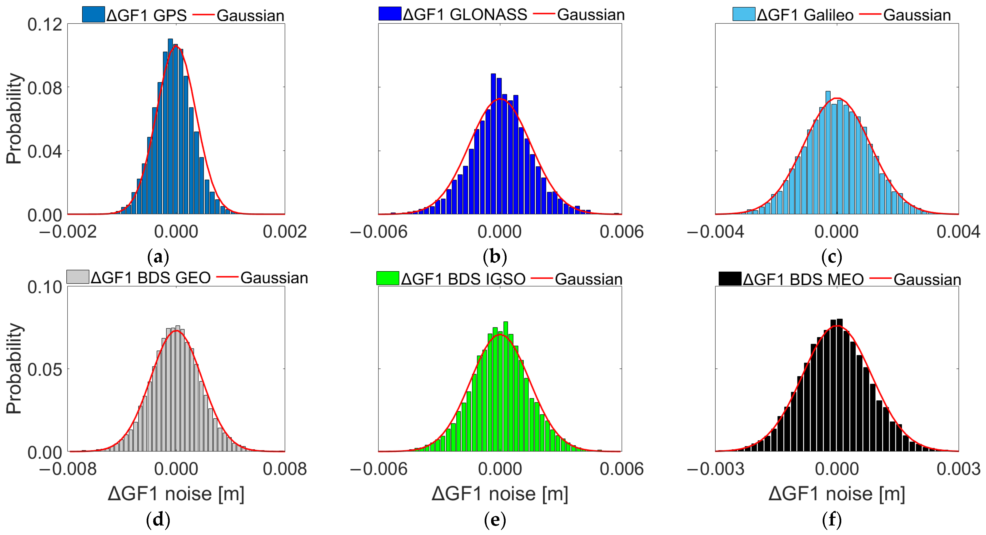
3.2. Distributional Characteristic Analysis on Gross-Error-Contaminated Observation Noise

The gross error simulations were introduced into the raw observations. According to the research by reference [1], in a typical city urban environment (Shanghai–Lujiazui area), 95% of the LOS multipath error lifetime is shorter than 13.6 s when the rover velocity is 0~3 km/h. Hence, the 10 s LOS multipath errors were introduced into the G08 raw observations from epoch 1801 to 1810. The LOS multipath errors are modelled as the observation noise variance jumps [4] as

$$\left\{\begin{array}{c}{P}_{k,r,j}^s=P_{k,r,j}^s+\mathrm{N}\left(0,{\left(15\mathrm{m}\right)}^2\right),1800<k\le 1810\\ L_{k,r,j}^s=L_{k,r,j}^s+\mathrm{N}\left(0,{\left(0.01\mathrm{m}\right)}^2\right),1800<k\le 1810\end{array}\right.$$

(12)

Moreover, reference [1] reveals that most LOS multipath errors are less than 350m, while the observations with much too large multipath errors are always eliminated by the a priori residual test (e.g., an empirical threshold 30 m) in PPP data pre-processing. Hence, a typical multipath standard deviation 15 m is selected to simulate the LOS multipath errors, which can pass the priori residual test. The phase tracking errors can be up to a quarter cycle (maximum 0.064 m for GPS L5, Galileo E5a, and BDS B2a and minimum 0.047 m for the last satellite in GLONASS L1 among all the systems). Consequently, introducing the 0.01 m phase variance jumps into the phase observations is a reasonable choice.

As for the NLOS reception errors, 95% of their lifetime is shorter than 68.2 s with 0~3 km/h rover velocity [1]. Hence, the NLOS reception errors can be modelled as the 60 s constant mean value jumps in the code and phase. However, $\Delta G{F}_{1,k,r}^s$ and $\Delta G{F}_{2,k,r,j}^s$ cannot extract the NLOS reception errors modelled as constant mean value jumps which are eliminated by the epoch-differenced strategy. Hence, only the LOS multipath errors are simulated to accomplish the analysis. The $\Delta G{F}_{1,k,r}^s$ PDF of G08, Student’s t distribution PDF ($\mathrm{DOF}=3$), and $\mathrm{N}\left(0,\mathrm{var}\left(\Delta G{F}_{1,k,r}^s\right)\right)$ are shown in Figure 3.

Figure 3 demonstrates that the distributional characteristics of the gross-error-contaminated observation noise can be divided into the Gaussian part and the heavy tail. When fitting the heavy tail, the Student’s t distribution with a proper DOF parameter is preferred to the Gaussian distribution. However, the Gaussian part is obviously better fitted by the Gaussian distribution than the Student’s t distribution. Hence, the Gaussian and Student’s t combined processing strategy will outperform to any single distribution-based strategy. Eventually, if the NLOS reception errors were introduced, the true distribution would obtain a heavier tail due to the mean value jump model.

4. Sequential Student’s t-Based Robust Kalman Filter

First, the robust Kalman filter and the Student’s t based Kalman filter (STKF) are introduced briefly. Then, the SSTRKF is derived by incorporating the RKF and the sequential Student’s t Kalman filter. Eventually, we provide the SSTRKF processing strategy.

4.1. Robust Kalman Filter Based on IGG-III Function

The RKF tunes the gross-error-contaminated observation noise in the standard Kalman filter by setting the robust factors as follows

$${\tilde{\mathit{Q}}}_k=\mathrm{diag}\left(r_{k,1},\dots ,r_{k,i}\right){\mathit{Q}}_k$$

(13)

where ${\tilde{\mathit{Q}}}_k$ is the new stochastic model with ${\tilde{Q}}_{k,i}=r_{k,i}{Q}_{k,i}$. $Q_{k,i}$ represents the $i$th element in the main diagonal of the raw observation stochastic model ${\mathit{Q}}_k$. $r_{k,i}$ is the $i$th observation robust factor, derived by the IGG-III function [30]

$$r_{k,i}=\left\{\begin{array}{cc}1& \left|{\overline{v}}_{k,i}\right|\le k_0\\ \frac{\left|{\overline{v}}_{k,i}\right|}{k_0}{\left(\frac{k_1-k_0}{k_0-\left|{\overline{v}}_{k,i}\right|}\right)}^2& k_0<\left|{\overline{v}}_{k,i}\right|\le k_1\\ \infty & \left|{\overline{v}}_{k,i}\right|\ge k_1\end{array}\right.$$

(14)

where $k_0$ and $k_1$ are presetting constants, chosen from 1.0 to 2.5 and from 3.5 to 8.0, respectively. The $i$th standardized residual vector ${\overline{v}}_{k,i}$ reads

$${\overline{v}}_{k,i}=v_{k,i}/\sqrt{Q_{v_{k,i}}}$$

(15)

where $v_{k,i}$ and $Q_{v_{k,i}}$ are the $i$th observation a priori residual and the corresponding variance, respectively. Note that $Q_{v_{k,i}}$ is the $i$th element in the main diagonal of the a priori residual covariance matrix ${\mathit{Q}}_{v_k}={\mathit{H}}_{y,k}{\overline{\mathit{Q}}}_k{\mathit{H}}_{y,k}^{\mathrm{T}}+{\mathit{Q}}_k.$ Here, ${\overline{\mathit{Q}}}_k$ is the covariance matrix of the one-step prediction ${\overline{\mathit{x}}}_k$. After redetermining the stochastic model of the observation system, the modified Kalman gain matrix can be written as

$${\overline{\mathit{K}}}_k={\overline{\mathit{Q}}}_k{\mathit{H}}_{y,k}^{\mathrm{T}}{\left({\mathit{H}}_{y,k}{\overline{\mathit{Q}}}_k{\mathit{H}}_{y,k}^{\mathrm{T}}+{\tilde{\mathit{Q}}}_k\right)}^{-1}$$

(16)

The RKF state estimators and the corresponding covariance matrices will be obtained after updating the Kalman gain matrix. As shown in Equation (14), the robust factors vary with ${\overline{v}}_{k,i}$ which is determined by $Q_{v_{k,i}}$ in Equation (15). Meanwhile $Q_{v_{k,i}}$ is significantly susceptible to the worse PPP/INS positioning solutions with poor satellite geometry.

4.2. Student’s t-Based Kalman Filter

The Student’s t distribution is applied to fit the gross-error-contaminated observation noise. The STKF can be described as follows [18,19]

$$\mathrm{p}\left({\mathit{x}}_k|{\mathit{y}}_{1:k-1}\right)=\mathrm{N}\left({\mathit{x}}_k;{\overline{\mathit{x}}}_k,{\overline{\mathit{Q}}}_k\right)$$

(17)

$$\mathrm{p}\left({\mathit{y}}_k|{\mathit{x}}_k\right)=\mathrm{St}\left({\mathit{y}}_k;{\mathit{H}}_{y,k}{\mathit{x}}_k,{\mathit{Q}}_k,{\vartheta }_k\right)=\int \mathrm{N}\left({\mathit{y}}_k;{\mathit{H}}_{y,k}{\mathit{x}}_k,\frac{{\mathit{Q}}_k}{{\xi }_k}\right)\mathrm{G}\left({\xi }_k;\frac{{\vartheta }_k}{2},\frac{{\vartheta }_k}{2}\right)\mathrm{G}\left({\vartheta }_k;p_k,q_k\right)\mathrm{d}{\xi }_k$$

(18)

where $\mathrm{St}\left({\mathit{y}}_k;{\mathit{H}}_{y,k}{\mathit{x}}_k,{\mathit{Q}}_k,{\vartheta }_k\right)$ denotes the Student’s t PDF with mean vector ${\mathit{H}}_{y,k}{\mathit{x}}_k$, scale matrix ${\mathit{Q}}_k$, and DOF ${\vartheta }_k$. ${\xi }_k$ is an auxiliary random variable obeying Gamma distribution $\mathrm{G}\left({\xi }_k;\frac{{\vartheta }_k}{2},\frac{{\vartheta }_k}{2}\right)$. The STKF adjusts the observation stochastic model mainly by ${\xi }_k$. Moreover, ${\vartheta }_k$ is also modelled as Gamma distribution with shape parameters $p_k$ and rate parameter $q_k$. The estimation problem can be solved by the VB method as follows [19]

$$\left\{q\left({\mathit{x}}_k\right),q\left({\xi }_k\right),q\left({\vartheta }_k\right)\right\}=\arg \min \mathrm{KLD}\left(q\left({\mathit{x}}_k\right),q\left({\xi }_k\right),q\left({\vartheta }_k\right)\left|\right|p\left({\mathit{x}}_k,{\xi }_k,{\vartheta }_k|{\mathit{y}}_{1:k}\right)\right)$$

(19)

where $q\left(\cdots \right)$ and $p\left(\cdots \right)$ denote the approximate posterior and posterior PDF, respectively. $\mathrm{KLD}\left(\cdots \right)$ is the Kullback–Leibler divergence. Equations (17) and (18) shows that the STKF simultaneously adjusts the stochastic model of every observation with solely one parameter ${\xi }_k$, which can mis-weight the gross-error-free observations. Moreover, the gross-error-contaminated observation noise has diverse stochastic characteristics, requiring separately processing. It is noticed that the computation burden of the STKF is relatively heavy as Equation (19) is solved iteratively. Although the Student’s t distribution degenerates to be Gaussian as the DOF tends to be infinite, conducting STKF with high-dimension matrices in every epoch can lead to disastrous computation burdens. Hence, the SSTRKF is proposed in the next section.

4.3. Sequential Student’s t-Based Robust Kalman Filter

The proposed SSTRKF first pre-weights the observations by Equation (14), which can give the proper observation noise covariance matrix with ideal satellite geometry and gross-error-free observation noise. Hence, after being pre-weighted by the IGG-III function, we conduct the chi-square test satellite-by-satellite as follows

$$\left\{\begin{array}{cc}{\left({\mathit{v}}_k^s\right)}^{\mathrm{T}}{\left({\tilde{\mathit{Q}}}_{v,k}^s\right)}^{-1}{\mathit{v}}_k^s\le th& H_0\\ {\left({\mathit{v}}_k^s\right)}^{\mathrm{T}}{\left({\tilde{\mathit{Q}}}_{v,k}^s\right)}^{-1}{\mathit{v}}_k^s>th& H_1\end{array}\right.$$

(20)

where ${\mathit{v}}_k^s$ and ${\tilde{\mathit{Q}}}_{v,k}^s={\mathit{H}}_{y,k}^s{\overline{\mathit{Q}}}_k{\left({\mathit{H}}_{y,k}^s\right)}^T+{\tilde{\mathit{Q}}}_k^s$ are the a priori residual vector and the corresponding IGG-III-modified covariance matrix of the satellite $s$, respectively. $th$ is the presetting chi-square threshold. Furthermore, $H_0$ and $H_1$ represent the null and alternative hypothesis, respectively. If the $H_0$ case is accepted, the IGG-III-derived variances of the satellite $s$ are reasonable. In contrast, the observations are sorted into the unreasonable variance group when accepting $H_1$. The reasonable variance group obeys the Gaussian assumption, whereas the unreasonable variance group is modelled by the Student’s t distribution. Hence, we first process the reasonable group by Equation (16).

The unreasonable group is sequentially processed due to the diverse stochastic characteristics of the gross-error-contaminated code and phase observations. Hence, the estimation problem of the unreasonable group can be presented as

$$\mathrm{p}\left({\mathit{x}}_{k,i}|{\mathit{y}}_{1:k-1},{\mathit{y}}_{k,\mathrm{N}},{\mathit{y}}_{k,\mathrm{ST},1:i-1}\right)=\mathrm{N}\left({\mathit{x}}_{k,i};{\overline{\mathit{x}}}_{k,i},{\overline{\mathit{Q}}}_{k,i}\right)$$

(21)

$$\begin{gathered} \mathrm{p}\left({\mathit{y}}_{1:k-1},{\mathit{y}}_{k,\mathrm{N}},{\mathit{y}}_{k,\mathrm{ST},i}|{\mathit{x}}_{k,i}\right)=\mathrm{St}\left({\mathit{y}}_{1:k-1},{\mathit{y}}_{k,\mathrm{N}},{\mathit{y}}_{k,\mathrm{ST},i};{\mathit{H}}_{y,k,i}{\mathit{x}}_{k,i},Q_{k,\mathrm{ST},i},{\vartheta }_{k,i}\right) \\ =\int \mathrm{N}\left({\mathit{y}}_{1:k-1},{\mathit{y}}_{k,\mathrm{N}},{\mathit{y}}_{k,\mathrm{ST},i};{\mathit{H}}_{y,k,i}{\mathit{x}}_{k,i},\frac{Q_{k,ST,i}}{{\xi }_{k,i}}\right)\mathrm{G}\left({\xi }_{k,i};\frac{{\vartheta }_{k,i}}{2},\frac{{\vartheta }_{k,i}}{2}\right)\mathrm{G}\left({\vartheta }_{k,i};p_{k,i},q_{k,i}\right)\mathrm{d}{\xi }_{k,i} \end{gathered}$$

(22)

where ${\mathit{y}}_{k,\mathrm{ST},1:i}=\left[\begin{array}{ccc}{y}_{k,\mathrm{ST},1}& \cdots & y_{k,\mathrm{ST},i}\end{array}\right]$ is the observation vector with the first $i$ observations in the unreasonable group. ${\mathit{y}}_{k,\mathrm{N}}$ denotes the reasonable variance group observation vector. Note that the subscript $i$ represents the $i$th observation in the unreasonable group. $Q_{k,\mathrm{ST},i}$ is the $i$th unreasonable observation variance, determined by Equation (13). Then, the estimation problem can be solved using the VB method as Equation (19).

The Gamma PDF $q^{\left(t+1\right)}\left({\xi }_{k,i}\right)=\mathrm{G}\left({\xi }_{k,i};{\alpha }_{k,i}^{\left(t+1\right)},{\beta }_{k,i}^{\left(t+1\right)}\right)$ is chosen as the posterior PDF for the auxiliary random variable ${\xi }_{k,i}$ in the $\left(t+1\right)$th iteration. Thus, the shape and rate parameter ${\alpha }_{k,i}^{\left(t+1\right)}$ and ${\beta }_{k,i}^{\left(t+1\right)}$ are derived as follows

$${\alpha }_{k,i}^{\left(t+1\right)}=\left\{dim+{\mathrm{E}}^{\left(t\right)}\left[{\vartheta }_{k,i}\right]\right\}$$

(23)

$${\beta }_{k,i}^{\left(t+1\right)}=0.5\left\{{\mathrm{E}}^{\left(t\right)}\left[{\vartheta }_{k,i}\right]+\mathrm{tr}\left[{\mathit{E}}_{k,i}^{\left(t\right)}{Q}_{k,\mathrm{ST},i}^{-1}\right]\right\}$$

(24)

$${\mathit{E}}_{k,i}^{\left(t\right)}={\left(y_{k,\mathrm{ST},i}-{\mathit{H}}_{y,k,i}{\widehat{\mathit{x}}}_{k,i}^{\left(t\right)}\right)}^2+{\mathit{H}}_{y,k,i}{\widehat{\mathit{Q}}}_{k,i}^{\left(t\right)}{\mathit{H}}_{y,k,i}^{\mathrm{T}}$$

(25)

where ${\widehat{\mathit{x}}}_{k,i}^{\left(t\right)}$ and ${\widehat{\mathit{Q}}}_{k,i}^{\left(t\right)}$ are the $t$th iteration estimator and the corresponding covariance matrix, respectively. $dim$ is the observation dimension. $\mathrm{tr}\left[\cdots \right]$ is the trace of a matrix. Furthermore, ${\xi }_k$ can be calculated through the expectation of the Gamma distribution as

$${\mathrm{E}}^{\left(t+1\right)}\left[{\xi }_{k,i}\right]={\alpha }_{k,i}^{\left(t+1\right)}/{\beta }_{k,i}^{\left(t+1\right)}$$

(26)

Another Gamma PDF $q^{\left(t+1\right)}\left({\vartheta }_{k,i}\right)=\mathrm{G}\left({\vartheta }_{k,i};p_{k,i}^{\left(t+1\right)},q_{k,i}^{\left(t+1\right)}\right)$ is exploited to be the posterior PDF of the DOF ${\vartheta }_{k,i}$, resulting in

$$p_{k,i}^{\left(t+1\right)}=p_{k,i}^{\left(0\right)}+0.5$$

(27)

$$q_{k,i}^{\left(t+1\right)}=q_{k,i}^{\left(0\right)}-0.5-0.5{\mathrm{E}}^{\left(t+1\right)}\left[\log \left({\xi }_{k,i}\right)\right]+0.5{\mathrm{E}}^{\left(t+1\right)}\left[{\xi }_{k,i}\right]$$

(28)

$${\mathrm{E}}^{\left(t+1\right)}\left[\log \left({\xi }_{k,i}\right)\right]=\mathsf{\psi }\left({\alpha }_{k,i}^{\left(t+1\right)}\right)-\log \left({\beta }_{k,i}^{\left(t+1\right)}\right)$$

(29)

where $\mathsf{\psi }\left(\cdots \right)$ denotes the digamma function. The expectation ${\mathrm{E}}^{\left(t+1\right)}\left[{\vartheta }_{k,i}\right]$ is obtained as

$${\mathrm{E}}^{\left(t+1\right)}\left[{\vartheta }_{k,i}\right]=p_{k,i}^{\left(t+1\right)}/q_{k,i}^{\left(t+1\right)}$$

(30)

Then, the posterior PDF of ${\mathit{x}}_{k,i}$ is modelled by the Gaussian PDF $\mathrm{N}\left({\mathit{x}}_{k,i};{\widehat{\mathit{x}}}_{k,i}^{\left(t+1\right)},{\widehat{\mathit{Q}}}_{k,i}^{\left(t+1\right)}\right)$. Thus, we obtain the measurement update process, given as

$${\tilde{Q}}_{k,i}^{\left(t+1\right)}=Q_{k,ST,i}/{\mathrm{E}}^{\left(t+1\right)}\left[{\xi }_{k,i}\right]$$

(31)

$${\mathit{K}}_{k,i}^{\left(t+1\right)}={\overline{\mathit{Q}}}_k{\mathit{H}}_{y,k,i}^{\mathrm{T}}{\left({\mathit{H}}_{y,k,i}{\overline{\mathit{Q}}}_{k,i}{\mathit{H}}_{y,k,i}^{\mathrm{T}}+{\tilde{Q}}_{k,i}^{\left(t+1\right)}\right)}^{-1}$$

(32)

$${\widehat{\mathit{x}}}_{k,i}^{\left(t+1\right)}={\overline{\mathit{x}}}_{k,i}+{\mathit{K}}_{k,i}^{\left(t+1\right)}\left(y_{k,\mathrm{ST},i}-{\mathit{H}}_{y,k,i}{\overline{\mathit{x}}}_{k,i}\right)$$

(33)

$${\widehat{\mathit{Q}}}_{k,i}^{\left(t+1\right)}={\overline{\mathit{Q}}}_{k,i}-{\mathit{K}}_{k,i}^{\left(t+1\right)}{\mathit{H}}_{y,k,i}{\overline{\mathit{Q}}}_{k,i}$$

(34)

More derivation details refer to references [18] and [19]. To intuitively demonstrate the process of SSTRKF, the flow chart is shown in Figure 4. Moreover, we elaborate the processing steps in the kinematic applications: (i) After the time update, the IGG-III pre-weighted observation stochastic model is calculated by Equations (12)–(14). (ii) The chi-square test is applied to sort the available satellites into the reasonable and unreasonable group. (iii) The measurement update with the Kalman gain obtained by Equation (16) is conducted for the reasonable group. (iv) The estimator and the corresponding covariance matrix of the reasonable group are assigned to ${\overline{\mathit{x}}}_{k,1}$ and ${\overline{\mathit{Q}}}_{k,1}$, respectively. (v) $p_{k,i}^{\left(0\right)}$ and $q_{k,i}^{\left(0\right)}$ are initialized by two presetting constants. (vi) Conduct the $i$th estimation by Equations (23)–(34). (vii) Assign ${\widehat{\mathit{x}}}_{k,i}^{\left(it{e}_{max}\right)}$ and ${\widehat{\mathit{Q}}}_{k,i}^{\left(it{e}_{max}\right)}$ to ${\overline{\mathit{x}}}_{k,i+1}$ and ${\overline{\mathit{Q}}}_{k,i+1}$, where $it{e}_{max}$ is the maximum iteration number. (viii) If $i$ is less than the unreasonable group observation number $N$, return to (v) with $i=i+1$. (ix) If $i=N$, output ${\widehat{\mathit{x}}}_{k,N}^{\left(it{e}_{max}\right)}$ and ${\widehat{\mathit{Q}}}_{k,N}^{\left(it{e}_{max}\right)}$ as the estimator and the corresponding covariance matrix of the current epoch.

5. Experiments and Discussions

The road experiments were conducted with SPAN-CPT IMU and a Trimble receiver in March 2019, Xuzhou, China. The dataset is available in the open-access software Ginav [31]. The experiment duration is 1721 s with 100 Hz IMU data and 1 Hz GNSS data. Note that we applied the RTK/INS tightly coupled solutions as the reference to evaluate the navigation performance. The precise clock and orbit products were obtained from the MGEX data-processing center (http://www.igs.org/mgex/products, accessed on 31 October 2021), and the satellite and receiver antenna parameters were gained from igs14.atx. In real-time navigation, the real-time clock and orbit products can be used to support PPP/INS.

Figure 5 is the 2D experiment trajectory, containing two laps on a same road. We select three segments of the road to conduct the six severe urban environment simulations, presented in red in Figure 5. To simulate the blockage urban environment as severe as possible, the cut-off elevation was set to 90° and 60° for the satellites with azimuth 285°~360° and 0°~285°, respectively. This environment can be always found in the urban environment, such as the narrow streets surrounded by high buildings. Moreover, the LOS multipath and the NLOS reception errors were introduced into an available satellite and the blocked satellite with the highest elevation, respectively. According to the analysis in Section 3.2, the lifetime and simulation model of the LOS multipath and the NLOS reception errors are summarized in

Table 1. The LOS multipath and the NLOS reception error simulation settings.

Simulation Number		1	2	3	4	5	6
LOS multipath error	Lifetime	10 s	10 s	0 s	0 s	20 s	10 s
	Model	$\left\{\begin{array}{c}{P}_{k,r,j}^s=P_{k,r,j}^s+\mathrm{N}\left(0,{\left(15\mathrm{m}\right)}^2\right)\\ L_{k,r,j}^s=L_{k,r,j}^s+\mathrm{N}\left(0,{\left(0.01\mathrm{m}\right)}^2\right)\end{array}\right.$
NLOS reception error	Lifetime	45 s	30 s	20 s	55 s	23 s	20 s
	Model	$\left\{\begin{array}{c}{P}_{k,r,j}^s=P_{k,r,j}^s+15\mathrm{m}\\ L_{k,r,j}^s=L_{k,r,j}^s+0.01m\end{array}\right.$

. It is noticed that the elevation of the satellite contaminated by the NLOS reception errors is higher than 50°, which tends to lead the NLOS reception errors lower than 50 m [1]. Therefore, the value of the NLOS reception errors was set to 15 m with the same consideration as the LOS multipath errors in Section 3.2.

The available satellite (AS) number of the multi-GNSS (GPS/GLONASS/Galileo/BDS), GPS (G), GLONASS (R), Galileo (E), BDS (C) is shown in Figure 6. During the experiment, the average AS number of multi-GNSS, G, R, E, and C are 18.9, 5.8, 2.5, 3.0, and 7.5, respectively. The first urban environment simulation was from 80 s to 125 s with 6, 1, 0, 1, and 4 average AS number for multi-GNSS, G, R, E, and C. During the 320 s~350 s, we conducted the second urban environment simulation, where the AS number drops to 4.3, 1, 0, 0, and 3.3 for multi-GNSS, G, R, E, and C on average, respectively. As for the third urban environment simulation during 540 s~560 s, the multi-GNSS, G, R, E, and C AS number maintain 4, 1, 0, 0, and 3, respectively. The fourth, fifth and sixth urban environment simulations were from 945 s to 1000 s, from 1227 s to 1260 s, and from 1445 s to 1465 s, respectively, where 4, 1, 0, 0, and 3 satellites for multi-GNSS, G, R, E, and C are available on average. Figure 6 indicates that the AS number reduces significantly during the urban environment simulations. Moreover, the shadow areas in Figure 6, Figure 7, Figure 8 and Figure 9 represent the urban environment simulations.

To reveal the impacts of the LOS and NLOS multipath errors on the positioning solutions in the urban blockage environment, we first conducted three schemes with the KF, summarized in

Table 2. Three simulation schemes to analyze the impacts of the urban environment.

	The LOS Multipath and NLOS Reception Errors	Blockage Environment
Scheme 1	No	No
Scheme 2	No	Yes
Scheme 3	Yes	Yes

. Figure 7 depicts the positioning errors of the three schemes, where the Scheme 1 achieves the best precisions among the three schemes. When suffering the blockage environment, the positioning errors (blue line in Figure 7) increases due to the barren observation conditions. Moreover, the positioning errors diverge dramatically when the LOS multipath and NLOS reception errors are introduced into the observations, such as the red line in Figure 7. Therefore, the gross errors induced by the LOS multipath effect and NLOS reception are rather serious problems for the PPP/INS tightly coupled system, especially in the urban severe blockage environment.

The chi-square test threshold was set to 13.277 with the significance level and the DOF being 1% and 4, respectively. Figure 8 gives the chi-square statistics during the road experiment. The chi-square statistics average 0.23 when neither the LOS multipath errors nor the NLOS reception errors are introduced. Moreover, only 15 in total 31,360 chi-square statistics exceed the chi-square threshold in this case, indicating that the IGG-III scheme can properly adjust the observation noise stochastic model in this case. On the contrary, the average chi-square statistics of the satellites impacted by the LOS multipath and NLOS reception errors are 41.6, 68.1, 89.3, 74.0, 52.8, and 72.0 for the six urban environment simulations, respectively. The chi-square statistics of the gross-error-contaminated satellites evidently exceed the chi-square threshold during the six urban environment simulations. Consequently, the IGG-III-based RKF fails to give proper variances for the gross-error-contaminated observations. Moreover, the SSTRKF avoids an unnecessary computation burden from processing every observation with the sequential Student’s t-based Kalman filter by dividing the observations into the reasonable and unreasonable variance group.

In the proposed SSTRKF, the sequential Student’s t-based Kalman filter is activated to process the observations that cannot be appropriately weighted by the IGG-III model. According to Section 4.3, $p_{k,i}^{\left(0\right)}$ and $q_{k,i}^{\left(0\right)}$ were initialized to 0.3 and 1 before processing every observation, respectively. The maximum iteration number of the SSTRKF was set to 10 [17,18,19]. To explore the superiority of the proposed SSTRKF, the KF, the RKF, the SSTRKF, and the STKF were applied to the multi-GNSS PPP/INS tightly coupled system in the Scheme 3 setting.

Figure 9 shows the KF, the RKF, the STKF, and the SSTRKF positioning errors during the road experiments. The STKF simultaneously tunes the observation noise covariance matrix with solely one factor, leading to the severely biased PPP stochastic model. Hence, the STKF errors diverge rapidly. It is evident that the positioning precisions are impacted by the urban environment simulation. The root mean square (RMS) positioning errors during the six urban environment simulations are collected in Figure 10. Compared with the KF, the proposed SSTRKF improves the horizontal and vertical precisions by 65.7% and 72.1% on average, respectively. Moreover, the SSTRKF achieves 57.5% and 62.0% average precision improvement relative to the RKF in the horizontal and vertical components, respectively. During simulation 2, although the RKF ameliorates the positioning precisions compared with the KF, the RKF positioning errors still diverge to 1.78m in maximum. As for the SSTRKF, the positioning precisions are improved by 29.4% and 32.6% relative to the RKF in the horizontal and vertical components during simulation 2. Moreover, the RKF impairs the positioning precisions compared with the KF during simulation 3, indicating that the RKF fails to derive proper observation variances with the IGG-III function. In contrast, during simulation 3, the SSTRKF suppresses the error divergence during simulation 3, reducing the horizontal and vertical positioning errors by 84.9% and 71.0% compared with the RKF and by 83.9% and 68.6% compared with the KF, respectively. In simulation 4, compared with RKF and KF, the horizontal and vertical PPP/INS precisions are improved by 80.3% and 95.3% and by 87.5% and 96.3% after applying the SSTRKF. As for simulation 5, the horizontal and vertical positioning errors of RKF and KF are reduced by 72.6% and 81.8% and by 54.2% and 76.7% with the SSTRKF. During simulation 6, the SSTRKF improves by 78.5% and 61.5% the horizontal and vertical positioning precisions compared with the RKF. As for KF, 89.3% and 76.7% horizontal and vertical precision improvement are achieved by conducting the SSRTKF. Moreover, the SSTRKF improves the positioning solutions slightly in the simulation 1. As shown in Figure 6, the observation condition of simulation 1 is better than the other five simulations, contributing to well-independent positioning. Hence, all three schemes can properly identify and handle the gross-error-contaminated satellites. According to the analysis above, the proposed SSTRKF evidently outperforms to the KF and RKF during the urban environment simulations, especially in the severe blockage environment.

6. Conclusions

The standard Kalman filter is optimal for PPP/INS tightly coupled only when the observation noise obeys the Gaussian assumption. However, the LOS multipath and NLOS reception gross errors in the urban environment lead to heavy tails in the observation noise. In the urban severe blockage environment, the heavy tails cannot be properly fitted by the IGG-III function. Hence, in this paper, we apply the Student’s t distribution to fit the heavy tails of the gross-error-contaminated observation noise. Moreover, the SSTRKF is proposed by sequentially conducting the RKF and the sequential Student’s t-based Kalman filter. The research findings and conclusions are summarized as follows.

• The GNSS phase and code observation noise obey the Gaussian assumption in the absence of the LOS multipath and NLOS reception errors. Moreover, the Student’s t distribution can fit the heavy tails of the gross-error-contaminated observation noise.
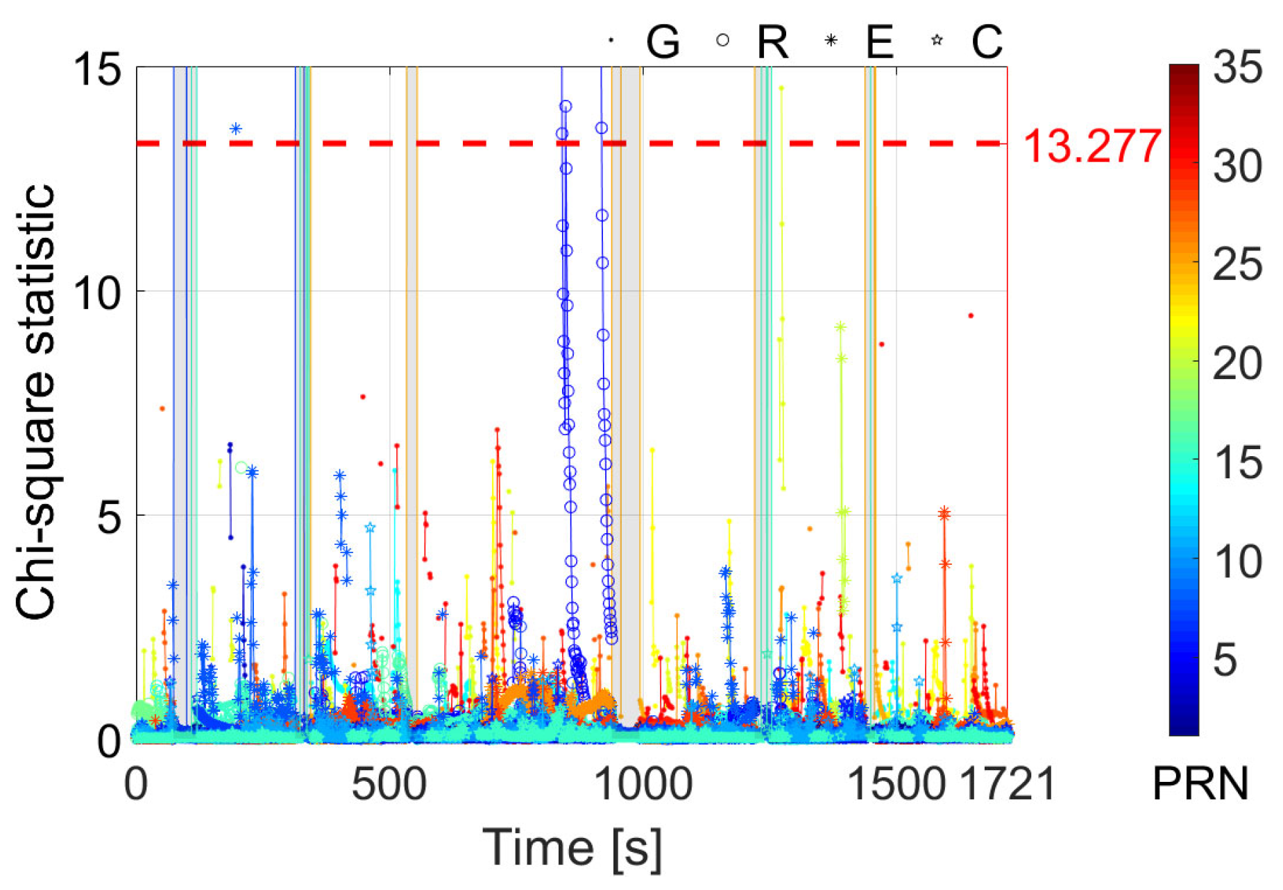
• The proposed SSTRKF can adjust the IGG-III function-derived unreasonable variances through the chi-square test and the sequential Student’s t-based Kalman filter, respectively.
• The numerical comparisons have validated our proposed SSTRKF for the gross-error-contaminated observations. Compared with the RKF, the proposed SSTRKF improves the horizontal and vertical positioning precisions by 57.5% and 62.0% on average during the urban environment simulations. Consequently, the proposed SSTRKF is superior to the KF and the RKF in the urban environment.

References

1. Chen, X.; Yu, J.M.; Yu, W.; Truong, T.K. GPS L1CA/BDS B1I Multipath Channel Measurements and Modeling for Dynamic Land Vehicle in Shanghai Dense Urban Area. IEEE Trans. Veh. Technol. 2020, 69, 14247–14263. [Google Scholar] [CrossRef]
2. Leick, A.; Rapoport, L.; Tatarnikov, D. GPS Satellite Surveying, 4th ed.; Wiley: New York, NY, USA, 2015. [Google Scholar]
3. Tang, W.; Wang, Y.; Zou, X.; Li, Y.; Deng, C.; Cui, J. Visualization of GNSS multipath effects and its potential application in IGS data processing. J. Geod. 2021, 95, 103. [Google Scholar] [CrossRef]
4. Spangenberg, M.; Calmettes, V.; Julien, O.; Tourneret, J.Y.; Duchâteau, G. Detection of variance changes and mean value jumps in measurement noise for multipath mitigation in urban navigation. Navigation 2010, 57, 35–52. [Google Scholar] [CrossRef] [Green Version]
5. Brodin, G.; Daly, P. GNSS code and carrier tracking in the presence of multipath. Int. J. Satell. Commun. 1997, 15, 25–34. [Google Scholar] [CrossRef]
6. Hsu, L.T.; Jan, S.S.; Groves, P.D.; Kubo, N. Multipath mitigation and NLOS detection using vector tracking in urban environments. GPS Solut. 2015, 19, 249–262. [Google Scholar] [CrossRef]
7. Groves, P.D.; Jiang, Z.; Rudi, M.; Strode, P. A portfolio approach to NLOS and multipath mitigation in dense Urban areas. In Proceedings of the ION-GNSS+−2013, Nashville, TN, USA, 16–20 September 2013; pp. 3231–3247. [Google Scholar]
8. Ng, H.F.; Zhang, G.; Hsu, L.T. A computation effective range-based 3D mapping aided GNSS with NLOS correction method. J. Navig. 2020, 73, 1202–1222. [Google Scholar] [CrossRef]
9. Wen, W.; Zhang, G.; Hsu, L.T. GNSS NLOS exclusion based on dynamic object detection using LiDAR point cloud. IEEE Trans. Intell. Transp. 2019, 22, 853–862. [Google Scholar] [CrossRef]
10. Hsu, L.T. Analysis and modeling GPS NLOS effect in highly urbanized area. GPS Solut. 2018, 22, 7. [Google Scholar] [CrossRef] [Green Version]
11. Atkins, C.; Ziebart, M. Effectiveness of observation-domain sidereal filtering for GPS precise point positioning. GPS Solut. 2016, 20, 111–122. [Google Scholar] [CrossRef] [Green Version]
12. Fuhrmann, T.; Luo, X.; Knöpfler, A.; Mayer, M. Generating statistically robust multipath stacking maps using congruent cells. GPS Solut. 2015, 19, 83–92. [Google Scholar] [CrossRef]
13. Chang, G. Robust Kalman filtering based on Mahalanobis distance as outlier judging criterion. J. Geod. 2014, 88, 391–401. [Google Scholar] [CrossRef]
14. Cheng, C.; Tourneret, J.Y.; Pan, Q.; Calmettes, V. Detecting, estimating and correcting multipath biases affecting GNSS signals using a marginalized likelihood ratio-based method. Signal Process. 2016, 118, 221–234. [Google Scholar] [CrossRef] [Green Version]
15. Guo, F.; Zhang, X. Adaptive robust Kalman filtering for precise point positioning. Meas. Sci. Technol. 2014, 25, 105011. [Google Scholar] [CrossRef]
16. Gao, Z.; Li, Y.; Zhuang, Y.; Yang, H.; Pan, Y.; Zhang, H. Robust Kalman filter aided GEO/IGSO/GPS raw-PPP/INS tight integration. Sensors 2019, 19, 417. [Google Scholar] [CrossRef] [PubMed] [Green Version]
17. Huang, Y.; Zhang, Y.; Li, N.; Wu, Z.; Chambers, J.A. A novel robust Student’s t-based Kalman filter. IEEE Trans. Aero. Elec. Sys. 2017, 53, 1545–1554. [Google Scholar] [CrossRef] [Green Version]
18. Huang, Y.; Zhang, Y. A New Process Uncertainty Robust Student’s t based Kalman Filter for SINS/GPS Integration. IEEE Access 2017, 5, 14391–14404. [Google Scholar] [CrossRef]
19. Wang, J.; Zhang, T.; Jin, B.; Zhu, Y.; Tong, J. Student’s t-based robust Kalman filter for a SINS/USBL integration navigation strategy. IEEE Sens. J. 2020, 20, 5540–5553. [Google Scholar] [CrossRef]
20. Zhang, B.; Hou, P.; Zha, J.; Liu, T. Integer-estimable FDMA model as an enabler of GLONASS PPP-RTK. J. Geod. 2021, 95, 91. [Google Scholar] [CrossRef]
21. Zhang, B.; Hou, P.; Zha, J.; Liu, T. PPP–RTK functional models formulated with undiferenced and uncombined GNSS observations. Satell. Navig. 2022, 3, 3. [Google Scholar] [CrossRef]
22. Zang, N.; Li, B.; Nie, L.; Shen, Y. Inter-system and inter-frequency code biases: Simultaneous estimation, daily stability and applications in multi-GNSS single-frequency precise point positioning. GPS Solut. 2019, 24, 18. [Google Scholar] [CrossRef]
23. Yan, G.; Weng, J. Strapdown Inertial Navigation Algorithm and Integrated Navigation Theory, 1st ed.; NPU Press: Xi’an, China, 2019. [Google Scholar]
24. Zhang, Z.; Li, B.; Shen, Y.; Yang, L. A noise analysis method for GNSS signals of a standalone receiver. Acta. Geod. Geophys. 2017, 52, 301–316. [Google Scholar] [CrossRef] [Green Version]
25. De Bakker, P.F.; Van Der Marel, H.; Tiberius, C.C.J.M. Geometry-free undifferenced, single and double differenced analysis of single frequency GPS, EGNOS and GIOVE-A/B measurements. GPS Solut. 2009, 13, 305–314. [Google Scholar] [CrossRef] [Green Version]
26. Zhang, X.; Li, X. Instantaneous re-initialization in real-time kinematic PPP with cycle slip fixing. GPS Solut. 2012, 16, 315–327. [Google Scholar]
27. Blewitt, G. An automatic editing algorithm for GPS data. Geophys. Res. Lett. 1990, 17, 199–202. [Google Scholar] [CrossRef] [Green Version]
28. Liu, Z. A new automated cycle slip detection and repair method for a single dual-frequency GPS receiver. J. Geod. 2011, 85, 171–183. [Google Scholar] [CrossRef]
29. Li, B.; Qin, Y.; Liu, T. Geometry-based cycle slip and data gap repair for multi-GNSS and multi-frequency observations. J. Geod. 2019, 93, 399–417. [Google Scholar] [CrossRef]
30. Yang, Y.; Song, L.; Xu, T. Robust estimator for correlated observations based on bifactor equivalent weights. J. Geod. 2002, 76, 353–358. [Google Scholar] [CrossRef]
31. Chen, K.; Chang, G.; Chen, C. GINav: A MATLAB-based software for the data processing and analysis of a GNSS/INS integrated navigation system. GPS Solut. 2021, 25, 108. [Google Scholar] [CrossRef]
Figure 1. Δ G F 1 , k , r PDF and N 0 , var Δ G F 1 , k , r of (a) GPS, (b) GLONASS, (c) Galileo, (d) BDS GEO, (e) BDS IGSO, and (f) BDS MEO.
Remotesensing 14 05878 g001
Figure 2. Δ G F 2 , k , r , 1 PDF and N 0 , var Δ G F 2 , k , r , 1 of (a) GPS, (b) GLONASS, (c) Galileo, (d) BDS GEO, (e) BDS IGSO, and (f) BDS MEO.
Remotesensing 14 05878 g002
Figure 3. Δ G F 1 , k , r s PDF of G08, N 0 , var Δ G F 1 , k , r s , and Student’s t PDF ( DOF = 3 ).
Remotesensing 14 05878 g003
Figure 4. Flow chart of the SSTRKF.
Remotesensing 14 05878 g004
Figure 5. Two-dimensional experiment trajectory.
Remotesensing 14 05878 g005
Figure 6. The AS number during the road experiments.
Remotesensing 14 05878 g006
Figure 7. Impacts of the LOS multipath and NLOS reception errors on the positioning solutions.
Remotesensing 14 05878 g007
Figure 8. Chi-square statistics during the road experiment.
Remotesensing 14 05878 g008
Figure 9. Positioning errors of the three filters.
Remotesensing 14 05878 g009
Figure 10. RMS positioning errors of the three schemes during the six simulations.
Remotesensing 14 05878 g010