1. Introduction
Road infrastructures are a vital part of our global transportation networks, both for general transit and freight. The pavement is one of the main assets, so it is necessary to perform frequent surveys to assess its general condition and identify possible distresses that could appear on it due to the passage of vehicles, climate action, and other potentially damaging phenomena. The infrastructure condition is also an important factor for road safety, as it is remarked by the European Commission [
1], which requests measures to be taken, including the implementation of regular and effective maintenance programs.
The most common type of road distresses are cracks, which can appear in longitudinal, transversal, or alternative directions relative to the traffic direction, or even create intricate patterns of intertwined smaller cracks, which is commonly known as alligator cracking [
2]. Other possible distresses to be found are rutting, potholes, the detachment of material, etc. Several approaches have been historically considered when tackling the issue of detecting pavement damage and are fundamentally different regarding the data acquisition techniques applied. Surveys have been traditionally performed relying on manual and visual techniques using simple measuring devices and carried out on-site, which tend to be time-consuming and costly, complicating the development of exhaustive and frequent monitoring routines, which are necessary for intensive coverage of the entire road network.
Remote monitoring techniques, however, offer faster and more complete solutions and even allow the automation of some of the tasks. These methods are used to configure a representation of the infrastructure through the acquisition of 2D images or 3D data, including structured light techniques and 3D laser scanning. Structured light consists of projecting a laser line on a surface and taking an image of it, capturing both the surface and the overlapped laser; this way, it is possible to establish a relationship between the pixels of the image and the range measurements of the laser, assigning depth values to them [
3]. Laser scanners can capture the whole scene in 3D by projecting laser beams in multiple directions. In the case of MLS (Mobile Laser Scanner) systems, as is used in this study, 3D scanning is achieved by combining the 360-degree rotation of a laser emitter with the movement of the vehicle, generating successive 2D scans that are then combined in a full 3D point cloud [
4].
While structured light is often employed for 3D road profiling and achieves good accuracy values, MLS allows for scanning not just the road but also its environment, including surrounding structures (bridges, tunnels, buildings, etc.), traffic signs, barriers, and other roadside elements. This way, it is possible to reuse the data acquired during the same survey for multiple purposes, including the evaluation of the pavement condition. This can also provide added value to information that was already acquired for a different task.
Multiple studies have been conducted employing remote monitoring technologies for distress detection from 3D road data. Some research has taken advantage of previously developed image processing techniques, applying them to raster images derived from point clouds. These are obtained by projecting the 3D point cloud onto a plane, which is divided into cells with a grid, which in turn correspond to pixels of an image. For instance, in [
5], Geo-Referenced Feature (GRF) images are generated using an Inversed Distance Weighed (IDW) rasterization algorithm, considering both intensity values of the points and their spatial distribution into the grid cell; then, an optimal threshold based on image histograms is used to select candidate crack points. A similar approach is developed in [
6] to extract cracks from walls scanned with the Terrestrial Laser Scanner (TLS), also using IDW rasterization on a Triangular Irregular Network generated from the point cloud. Chen and Li [
7] apply voxelization during the pre-processing step on the point cloud to generate a Digital Terrain Model (DTM) and segment the ground; a raster of the DTM is obtained by assigning the minimum height within a grid cell to each pixel, and a high-pass filter is applied to detect local elevation changes and identify candidate crack areas. Point cloud voxelization was also employed as a preliminary step to apply image classification techniques by Cho et al. [
8]. Instead of using the original points’ elevation values to identify distresses, De Blasiis et al. [
9] proposed using roughness values, calculated as the distance from a certain point to a plane adjusted to its neighbors; a Digital Elevation Model (DEM) raster was then constructed, assigning roughness values to the pixels. Another way to arrange the point cloud into a grid pattern was introduced by Zhong et al. [
10] using the scanning angle and the scanning line number provided by a 2D laser scanner.
An alternative to image processing tools is to combine 2D images and 3D data to produce enriched models of the ground, complementing the information provided by each data type. Some data fusion methods are Bayesian, the fuzzy logic method, or the Dempster–Shafer theory [
11], which allows the combination of imprecise and incomplete information from different sources to improve the results. In this case, 2D grayscale images and laser scanner lines are combined to detect cracks, based on both the elevation and intensity differences between points. Another possibility is the preliminary adaptation of acquired data with different sensors to increase coherence; for example, Chen et al. [
12] proposed merging 2D grayscale images with depth images of concrete surfaces; the depth images were obtained by transforming the coordinates of 3D point clouds to a fitting plane calculated via PCA (Principal Component Analysis). This way, the data fusion is realized at a pixel level, improving both crack saliency and background noise reduction and allowing the use of a crack segmentation technique based on Otsu thresholding. Following a different approach, Valença et al. [
13] proposed using a reconstructed 3D model from point clouds with pre-selected targets on it to serve as a pattern for the rectification of images. This allowed the identification of discontinuities through an intensity filter; geometric data were utilized to further identify discontinuities (mainly cracks) based on the orthogonal distance of surface points of the model to a PCA-calculated plane.
The works cited above mainly focus on using image analysis techniques or enriched models combining images and 3D laser scanner data. However, road distress can be detected and extracted directly from 3D point clouds, based on the geometric and radiometric information contained in them. Tsai and Li [
14] evaluated the feasibility of detecting cracks from 3D laser-profiler data by comparing the results of crack segmentation via the dynamic-optimization algorithm [
15] with ground-truth images. Another common approach is to extract transversal road profiles from the 3D point clouds for their study, focusing on the high-frequency components of the profile to measure roughness and check for cracks in the form of strong elevation changes (or other indicators). In [
3], these high-frequency components were detected by applying the Haar Transform (a type of wavelet transform) in search of crack edges. Gui et al. [
16] applied a high-pass filter and the CFAR (Constant False-Alarm Rate) to obtain candidate crack seed areas, considering each set of connected points as an object with depth, geometric, and topological features. Li et al. [
17] used the Fast Fourier Transform (FFT) to convert the profile signal into the frequency domain and then separate the pavement texture containing crack components from the main shape profile, also applying an elevation difference threshold to detect potential crack points and generate a binary map. Zhou et al. [
18] also decomposed the pavement in low-frequency, sparse, and texture components. Instead of applying frequency decomposition, Ravi, Bullock, and Habib [
19] analyzed individual MLS scanning lines by partitioning them into shorter segments of 1 m to find distress seed points that deviate from the best fitting line; additional points that deviate from the best fitting plane of the seed neighborhood were marked as additional distress points. Other studies focus on modelling cracks mathematically to determine their severity levels and the causes behind them based on their properties, such as the crack width, total length, or crack intersection points [
20]. For instance, Yang et al. [
21] compared the crack length growth between sealed and non-sealed sections of roads to quantify the benefits of crack sealing. A different approach was followed by [
22], using a space mapping strategy to enhance intensity differences and distribution structure distinctions of crack points, relying then on a GCN (Graph Convolutional Networks) semi-supervised algorithm to detect the cracks. Additional types of distress can also be detected from 3D laser data. El Issaoui et al. [
23] detected rut vertices on scan profiles with a convex hull and then measured the distance of rut points to the ideal road line.
The next step after the candidate crack points selection is to cluster them and extract the cracks themselves. In the aforementioned work from Gui et al. [
16], lower and larger objects (clustered point sets) are merged based on their orientation and the distance between them, selecting those fitting typical crack parameters as crack seeds and employing tensor voting to create a crack probability map. Zou et al. [
24] followed a similar approach to create a crack probability map from grayscale images acquired with structured light techniques, using path voting to result in a graph describing possible connections between cracks and selecting the most feasible ones via a Minimum Spanning Tree (MST). In [
17], crack seeds obtained from a binary map were connected according to the Gestalt laws of proximity, similarity, and continuity, extracting paths via MST as well. In both [
25] and [
26], the authors used a convex hull to delineate individual defects, although, in the latter, a variant of the method known as alpha-shapes was used, which does not limit the resulting perimeter of the crack to a convex shape. Zhou et al. [
18] used the TUFF (Tubular Flow Field) algorithm to delineate cracks. Other methods to extract cracks include the use of Euclidean distance clustering and L1-median filtering [
27] or Iterative Tensor Voting (ITV), which produces a refined crack probability map enhancing crack pixels and suppressing the background and noise [
28].
Although most of the available research relies on data acquired with highly accurate laser profilers [
3,
14,
16,
17,
18,
21], the use of MLS point clouds provides more versatility compared to these instruments because the whole road environment is recorded by the mobile laser scanner. This way, the same survey operation can serve multiple purposes without employing additional sensor systems, allowing us to make the most of data that could have been recorded for a different reason; for instance, point clouds of the dataset introduced in this research were originally obtained for road inventory purposes. Therefore, we propose a methodology to detect, extract, and parametrize severe cracks on road pavements from 3D point clouds acquired with MLS technology relying only on geometrical data. First, the pavement is segmented from the point cloud and samples of it are selected. These samples are further divided into individual scanning lines to obtain road bidimensional profiles, which are filtered to isolate the higher frequencies of the profile and then apply a variable threshold based on point elevation for the detection of candidate crack points. As intensity information is not needed for crack point detection, this avoids possible irregularities due to differences in materials, temperatures, or moisture levels across the inspected surface [
29,
30]. A region-growing algorithm has been developed from scratch to cluster together the crack points and thus create crack sections, which are further merged into bigger ones. Several geometrical parameters of the cracks, such as their length, width, or area, are calculated to measure the extent of pavement affected by cracking.
There are other methods relying on MLS point cloud data to detect cracks on pavements, using image segmentation to extract results from images constructed from GRF [
5], DTM [
7], or DEM [
9] raster data, as mentioned above. Instead of following a similar approach, our method works directly with the 3D point cloud data (after segmenting the ground), which allows it to retain its original geometry, as no process of rasterization, voxelization, or any kind of interpolation is performed during the crack detection and extraction. This allows us to measure all the geometric parameters for the extracted cracks directly on the point cloud, preserving its shape, resolution, and precise location of the points. Original 3D point cloud data were also used in [
19], differing in the candidate distress point identification strategy at the individual scanning line level and limiting the scope to the distress point detection without clustering or extracting the distresses themselves. To summarize, our research proposes the following contributions:
Detection of candidate crack points from MLS data at an individual scanning line level using variable thresholding based on point elevation standard deviation.
Extraction of cracks directly from the 3D point cloud data based on a region-growing algorithm developed from scratch.
Parametrization of the extracted cracks, measuring all dimensions directly on the original point clouds.
Establishment of the basis for a quick pre-rating tool for pavement condition based on the detected crack area.
This paper is organized from this point forward as follows: In
Section 2, we introduce the case study, the equipment employed, and a detailed description of the methodology.
Section 3 includes the experimental results and their discussion. Finally, the conclusions of our research are explained in
Section 4.
2. Materials and Methods
The MLS employed for the data acquisition in this study was an Optech Lynx Mobile Mapper M1, including two LiDAR sensors capable of rotating at up to 200 Hz, thus completing 200 scanning cycles per second [
31]. This system has a laser measurement rate of up to 500 kHz with each LiDAR sensor, achieving a range measuring precision of 8 mm. The navigation system was provided by Applanix [
32] and included an INS, two GNSS antennas, and an odometer. For this study, we set the scan frequency to its maximum of 200 Hz, and the laser measurement rate was at 250 kHz in both sensors. The scan produced during a single revolution of one sensor contained 1250 points, resulting in an angular resolution of 0.288-degree; this equates to separation between points within the same scanning line of approximately 13 mm at a range of 2.5 m, which is approximately the orthogonal distance from the LiDAR sensor to the pavement surface. This was validated by computing point separation in actual point clouds, which showed a resolution of 14 mm for points close to the scanner and 74 mm at the verge of the roadway, with approximately 90 mm separation between scanning lines (this value is dependent on the speed of the vehicle). Therefore, the minimum detectable crack width was limited by that point resolution for cracks that are fully or partially transversal to the scanning lines, and it increased at locations that were further away from the scanner, coinciding with the findings of Laefer et al. in [
33]. Cracks parallel to the scanning lines were omitted by the algorithm unless they were wide enough to overcome the big gaps between consecutive scanning lines. These specifications contrast with those of a typical dedicated 3D laser road profiler, such as the one used in [
18], which offers much better resolution within a scanning line with 1 mm of point separation and 1–5 mm between consecutive lines, so employing an MLS limits the magnitude of the cracks that can be detected in the point clouds.
The case study consisted of a dataset that included point clouds and images acquired along a 5 km section of a ring road of a Portuguese town that was inspected by the infrastructure manager in 2018, evaluating its condition as deficient based on criteria such as the calculated IRI (International Roughness Index) or the percentage of the cracked area measured, for instance.
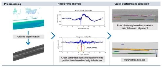
The method constitutes several steps, including pre-processing tasks to segment the ground part of the point cloud and divide it into individual scanning lines as recorded with each full rotation of the laser scanner. After this, road profiles derived from those scanning lines were analyzed to obtain candidate crack points (referring to those segmented from the ground point cloud), which were then clustered together in separate cracks considering their neighborhood.
2.1. Candidate Crack Point Detection
2.1.1. Point Cloud Pre-Processing
The original point cloud contains comprehensive information about the surroundings of the survey vehicle, but only data regarding the ground part of the cloud is relevant for the present study, so the first step consisted of isolating it. The point cloud was initially voxelized using a 5 cm voxel size, which allowed for capturing enough points on the road and its near surroundings, and the survey vehicle trajectory data were used as assistance. A ground segmentation function based on a region-growing algorithm inspired by Douillard et al. [
34] selected those voxels that were closer to the trajectory of the survey vehicle as seeds. Then, the neighborhood of each seed voxel was studied, and voxels with mean heights and height variances (equal to the standard deviation of the neighborhood point set) similar to those of the current seed were added to the ground cluster. Then, indices of points belonging to the ground were retrieved from the corresponding ground voxels, allowing the segmentation of the point cloud [
35]. However, points along the verges of the ground cloud were not evenly distributed, which could be observed by the reduced number of points with scanning angle values highly deviating from the mean of the whole set. Therefore, only points with a scanning angle within a range of ±1.5 times the standard deviation were accepted, which was proven to retain the whole driving area for the entire length of the scanned road while avoiding the irregular verges at the same time.
2.1.2. Road Profile Analysis
Each time the mirror of the LiDAR sensor employed for this research completed a 360-degree rotation, it produced a scan containing all the points recorded by each of the laser beams projected during that rotation. Once the ground was segmented from the original 3D point cloud, these individual scans were represented by lines of points on the pavement, spaced apart according to the speed of the vehicle. These lines could be isolated by sorting the points according to their timestamp and relying on their scanning value, as it resets with every new scanning cycle. Each scanning line was then transformed to better interpret the shape of the corresponding road profile and evaluate its roughness components in the search for candidate crack points, as shown in
Figure 1.
To adapt points of a single scanning line (
Figure 2a) to a 2D space, PCA was applied for its x, y, and z coordinates to determine the first principal component of the point set, which represents the distribution of the points across the scanned road section. The 2D representation of the points (
Figure 2b) is expressed based on that first principal component and the original Z coordinate (point elevation). PCA was then applied on the 2D set of points to obtain the oscillation in point elevation across the scanning line and suppress the effect of the road slope (
Figure 2c).
The resulting pavement profile not only contains information about the pavement texture and possible cracks present on it but also the general shape of the surface. Therefore, the profile, handled as a spatial domain signal comprised of a discrete number of points (n), was decomposed according to its spatial frequency distribution using the Discrete Fourier Transform (DFT) [
36], given by Equation (1).
This function mapped the elevation values of vector
to the frequency domain vector
, which represents the Fourier coefficients, both comprising n elements. Each
-th element of the frequency domain data vector
was calculated as the sum of
products of the
-th element of elevation vector
and an exponential function. The argument of this exponential function results from multiplying the
and
indexes of each iteration, the
number of elements in the vectors, and the number
(pi). The DFT was implemented much more efficiently using the FFT, reducing the number of operations involved from
to
by reorganizing the terms of the input vector
and the DFT linear operator. The power spectrum of the signal was calculated using the Fourier coefficients so the signal can be represented as a function of the spatial frequency, indicating how much power corresponds to each frequency (
Figure 3a). As lower frequencies associated with the general shape/undulation of the road section show much higher power than higher frequencies, the use of a low-pass filter is straightforward regarding isolating those lower frequencies. Then, the Inverse Fast Fourier Transform (IFFT) was used to obtain the corresponding road undulation signal (
Figure 3b). The difference between the original road profile and this undulation profile was computed, obtaining the roughness/texture profile (
Figure 3c).
2.1.3. Crack Points Detection
Candidate crack points were selected as those with an elevation value above a threshold that was individually set for each road profile. First, the elevation standard deviation (
) was calculated according to Equation (2), with
being the number of points in the profile,
being the elevation value of each point, and
being the mean elevation of the profile. The detection threshold was defined as the sum of the mean profile elevation and the elevation standard deviation multiplied by a factor of
, as represented in Equation (3), which was adjusted based on empirical experimentations. The aim was to detect enough points belonging to cracks to accurately delineate them while maintaining a reduced level of noise due to false positives. An initial threshold of 2 times the standard deviation (
) was trialed on one of the sections of the road to be tested, allowing us to almost completely retain the shape of the cracks but with a very high level of noise that made their extraction difficult. Upon increasing the threshold to
the noise was greatly reduced, but so was the density of points in the crack areas, although their shape was still correctly retained. Thus, an intermediate threshold value of
was applied for all the scanlines through the various road sections tested.
2.2. Crack Clustering
Since the set of candidate crack points detected with the proposed method is noisy and cracks do not appear completely delineated, it is necessary to remove outliers and group the remaining valid points in crack clusters. To do so, an approach based on the DBSCAN clustering algorithm [
37] was investigated, but the results were not optimal due to the density-based nature of the algorithm. Therefore, a point region-growing algorithm was developed, which selects a seed point to start a cluster and then adds subsequent points based on their proximity, orientation, and alignment between points. Once a cluster is completed, or if the point selected to act as the seed is discarded as noise, the algorithm continues iterating until all candidate crack points are labelled.
Figure 4 describes how the algorithm operates.
First, PCA was applied to the coordinates of the original pavement point cloud to calculate its eigenvectors, so a change of basis could be performed on the crack points to project them onto the plane that best fits the pavement section. Feasible seed points were determined by selecting those with enough neighbors within a given search radius. The search radius and the minimum acceptable number of neighbors were adjusted to filter out noisy points initially identified as cracks (
Section 2.1.3), using the same test pavement section. It was found that a 0.6 m radius and 5 neighbors were the best-performing values, retaining enough crack points but rejecting isolated ones. A bigger search radius (~1 m) and a smaller number of required neighbors were found to be insufficiently restrictive, while the opposite approach omitted valuable crack points. Once the valid seed points were selected, the orientation of all of them was calculated by selecting the retrieved neighbors of a given point and applying PCA to them, selecting the first eigenvector of each set. The direction angle of the point (
) was calculated from the two first components (
,
) of that first eigenvector, as detailed in Equation (4).
The next step consisted of an iterative method to group points in different clusters. In each iteration, a seed point was selected from those that were still not assigned to a certain cluster or labelled as noise, and a new cluster was started. A range search was used to determine the neighbors of the seed point, and both the direction of the neighbors and the angle of the lines connecting each of them with the seed point were compared with the direction of the seed point (
Figure 5a,b). If the difference between the direction of the seed point and that of a given neighbor was within the established angular thresholds (±dir_diff), both points were considered to have compatible directions (
Figure 5c). Likewise, if the difference between the direction of the seed point and the orientation of the line connecting it to a given neighbor was within the corresponding angular thresholds (±alig_diff), both points were considered to be aligned (
Figure 5d). Points that meet both conditions (compatible directions and alignment) were labelled for the same crack point cluster. After empirical testing, the best thresholds for direction similarity and alignment between points were found to be ±12 and ±15 degrees, respectively, achieving clusters that adapt to the shape of the cracks and do not contain high levels of noise. During these tests, when applying narrower angles (10 degrees or less), the resulting clusters were smaller and disconnected, while wider angles (20–30 degrees) allowed the creation of clusters from seed points that did not show significant alignment or orientation coherence with their neighbors, instead of focusing on the bigger, most relevant groups of points. Both angles were modified together until reaching acceptable results and then slightly adjusted at an individual level. To avoid overfitting, the aim of adjusting these parameters was limited so enough information about visible cracks on the road could be retained while reducing the noise level as much as possible.
If there were not any neighbors that meet these criteria, the seed point was labelled as noise and the current cluster was discarded; otherwise, the neighbors that were further from the seed point in both directions along the X-axis of the plane were selected as the new seed points, if they had enough neighbors themselves, to continue growing the cluster. Once no more suitable points were found, the cluster was finished and a new one was started; this process was repeated until all candidate crack points were either included in a certain cluster or labelled as noise.
Geometrical parameters were calculated for the clusters, such as the number of points they contain, point density, and linearity (Equation (5), calculated as the difference between the two first eigenvalues (
and
) and divided by the first one), so those clusters that do not comply with specified thresholds can be filtered out. The same control pavement section point cloud was used to determine the most suitable values for these thresholds, establishing a minimum of 7 points per cluster, a point density higher than 15 points per square meter, and a linearity over 0.98. The reason for using these specific thresholds is to avoid non-relevant clusters (with few or dispersed points) and focus on large, linear cracks.
The connectivity between clusters was assessed to further group the filtered crack points into larger clusters. To accomplish this, each cluster was represented as a simple graph with two vertices (both extreme points along the principal direction of a cluster) and an edge connecting them (
Figure 6). In a similar manner as the process of initially clustering together the candidate crack points, the proximity, similar orientation, alignment, and overlay between each possible couple of clusters were analyzed to evaluate their compatibility. For instance, to determine the proximity, the length of all edges connecting pairs of vertices from two different clusters was calculated, and the shorter edge was selected (
Figure 7). The orientation of this edge was compared to that of the two clusters it is connecting to assess the alignment between them; the orientation difference between the two clusters was evaluated too. Finally, the area of each cluster was measured with a convex hull enclosing its points, projected onto the pavement plane, and the intersection of areas between two clusters was measured to check overlays. The
adjacency matrix was generated for each of these four parameters, with
being the number of clusters, to summarize connectivity between them. If a pair of clusters was compatible according to the threshold applied for each parameter, a true value was assigned in the corresponding place of that adjacency matrix. All clusters that were overlayed, or at the same time were close, similarly oriented, and aligned, were considered connected (
Figure 8). The overlaying threshold was set at 15%, the maximum distance between clusters limited at 2 m (to maintain cracks with large gaps in between separated from each other), and alignment and orientation angular differences between clusters were set to double those used for individual points (±30 and ±25 degrees ranges, respectively) to relax the criterion because irregular or incompatible clusters were already filtered out in previous steps of the method.
2.3. Crack Parametrization
After grouping crack point clusters according to the established connectivity conditions, geometric parameters of each crack point cluster were computed, namely the number of points in the cluster, its length, width, orientation, and the area calculated both via convex hulls and alpha-shapes, which is a “generalization of the convex hull of a point set” [
34] that is not necessarily convex or connected. The length of each crack, calculated between the most distant points along the main direction of the point cluster, was used as the main indicator of its magnitude, together with the area calculated according to its convex hull.
3. Results and Discussion
The proposed crack detection methodology was evaluated using point clouds and images from the aforementioned Portuguese road dataset. A visual inspection was carried out on the 360-degree camera streams, and four sections of pavement were selected at different spots in the road to mark the location of the largest cracks on the pavement (
Figure 9), as well as other areas less severely affected by cracking but still visually damaged. These regions of the pavement were then manually sketched on top of the MLS point clouds in an attempt to match what was marked on the images by roughly delineating the boundaries of the area of interest and then segmenting the points contained inside for each individual marked distress. To achieve this, the intensity value of the points in the cloud was used to identify the same features of the road as distinguished in the images. Due to the limitations of this procedure, an accurate ground truth could not be established. Instead, the length and area of the detected crack clusters were compared to those of manually segmented regions at coinciding locations, to assess if distresses that are visible in the images were correctly identified and located by the method.
In the first spot, crack clusters detected with the automatic method (
Figure 10) realistically reflect the situation that can be observed in the images (
Figure 9). The longitudinal crack along the central road line is divided into two sections (clusters marked as 1 and 2 in the image), missing the area on top of the painted line, likely because the damage appears to be less severe in that area. The right lane crack also appears almost completely (clusters 3 and 4) except for, again, a small section of points in the middle. Thinner cracks between the larger ones (circled in blue in
Figure 9) are either not detected when identifying candidate points or filtered out during the clustering process.
Comparing the cracks detected by the proposed method with those manually segmented, both sets show great similarities. The two longitudinal cracks detected at the centerline of the road cover 89% of the total length of the manually segmented area, marked in dark grey in
Figure 11; in the case of detected cracks at the center of the right lane, this indicator is reduced to 80%. Regarding the small crack in the left lane, the detected crack cluster (marked as 5) covers 79% of its length. The transversal line that delimits the pass from the repaved section of the road in the right lane to the worn section (cluster 6) is only partially detected (36% of its length), likely because the crack point detection algorithm aims to select points with prominent, negative elevation values; this line could be better described as a step rather than a crack and points in the area can stand out either by too high or low elevation values, so the partial detection achieved is in line with this assumption.
The second spot presents the same longitudinal crack all along the centerline between lanes, with the rest of the pavement being affected by lighter cracks, especially on its right side, as can be observed in
Figure 12 (slightly cracked pavement circled in blue). The centerline crack was correctly identified; on the other hand, light cracks are merely detected and represented by small, scattered clusters, and a small crack located in the left lane was missed too. This should be expected considering the resolution of the MLS employed, with a minimum of 13 mm of separation between points of the same scanning line near the sensor, which increases to 74 mm at the left verge of the road (the furthest location from the sensor) and a resolution of 90 mm between lines, as indicated in
Section 2. Therefore, only the centerline crack was considered valid at this spot, comprised of the three numbered crack clusters in
Figure 13. Adding up the longitudes of these three in-line crack clusters, the longitude covered matches 93% of that of the manually segmented area, marked in dark grey in
Figure 14; the other cracks, considering their relatively reduced magnitude, were not marked because scattered crack point clusters detected by the method do not match any specific distress identified by visual inspection.
The third spot presents a complex layout (
Figure 15), with larger cracks and smaller, intricate ones, describing an alligator cracking pattern. The method detects the bigger ones, including the centerline crack (clusters numbered 1 and 2 in
Figure 16) and a series of successive cracks at the right side of the right lane (cluster 3, continued by cluster 4 after an interruption) although, again, smaller cracks are missing. The detected crack points cover 98% of the length of the centerline crack (
Figure 17). Two smaller cracks by its side (cluster 5 and the combination of 6 and 7, respectively) were also captured, both covering over 70% of the length of the corresponding manually segmented areas. Only sparse points of the alligator cracking area marked in blue in
Figure 15 were found, so the detection of those cracks was not taken into account.
The last spot presents a repaved area that interrupts the centerline crack, and a big, wide crack crossing the road diagonally (
Figure 18) produced by the separation of the deck of the road at that point. The severity of the centerline crack is reduced in this part of the road, being merely visible in the images at some points and completely interrupted once the road reaches the repaved area. The proposed algorithm can capture this, recognizing only the most severely affected areas, as can be observed in
Figure 19, with clusters number 1 and 2 representing the visible part of the crack before and after the repaved section of the road, respectively. A narrower crack on the right lane was not captured by the algorithm. The detected diagonal crack (cluster 3) covers 79% of the segmented area (
Figure 20).
In
Table 1, the cracks that were correctly identified (considering both bigger cracks and lighter alligator cracking areas) by the algorithm against the total number of manually identified cracks are presented; in general, severe cracks manually segmented are correctly identified by the algorithm, although they can be partitioned into several pieces if the degree of the damage is not continuous. Some minor cracks (mentioned above for the case studies of spots 1 and 4) were missed, and the areas affected by alligator cracking could not be correctly detected due to the reduced severity of the damage and their intricate patterns.
Table 2 compares the crack clusters that the algorithm detected correctly with the corresponding manually segmented regions of pavement. Multiple algorithm cracks related to the same manual region are merged by calculating the union of their convex hull polygons. The intersection and union of the resulting algorithm crack region with the corresponding manual region are obtained, and the ratio between both areas is found. The same ratio is calculated for the perimeter of the intersection and union of regions because, considering the slim shape of cracks, a small difference in the width of comparable regions is translated into a big difference in terms of area. Results show how, in general terms, detected cracks coincide with the manually segmented regions, especially regarding the perimeter values. However, it would not be feasible to assess the accuracy of the crack extraction based on these metrics because of the subjective nature of the ground truth presented, as manually outlined regions may not adjust to the real damaged road area. Due to this, these results must be considered as an indicator of the capability of the method to identify and locate severe cracks but not to extract them fully and accurately as this could not be assessed with the current dataset.
Other geometric parameters are calculated for all individual crack clusters identified with the method, namely their length, width, CH (convex hull) and alpha-shape areas, and their orientation relative to the principal direction of the evaluated road segment/spot. In
Table 3, the parameters corresponding to the first road spot analyzed are shown as an example. These attributes could allow the identification of the most relevant distresses that the algorithm can detect and their classification based on diverse criteria, e.g., longitudinal/transverse cracks according to their orientation, linear/widespread defects depending on the relationship between the length and width, etc. The ratio between the area covered by the set of cracks identified in each road spot and the total area of pavement is calculated to obtain the percentage of the cracked area of the pavement at each spot, as shown in
Table 4. This metric could be used as a preliminary indicator of the general state of the section of pavement surveyed, regarding the presence of cracks. As we can see, the result for the total affected area identified by the algorithm is similar to that manually delimited; there are slight differences but the magnitudes match. Regarding computing performance, the method is not time consuming, as we were able to execute the algorithm and process each road spot in just a few seconds using a regular laptop computer, so average hardware should be enough to meet the requirements.


