Article

A Novel Fully Coupled Physical–Statistical–Deep Learning Method for Retrieving Near-Surface Air Temperature from Multisource Data

1
School of Surveying and Geo-Informatics, Shandong Jianzhu University, Jinan 250100, China
2
Institute of Agricultural Resources and Regional Planning, Chinese Academy of Agricultural Sciences, Beijing 100081, China
3
School of Physics and Electronic-Engineering, Ningxia University, Yinchuan 750021, China
4
School of Public Administration and Law, Northeast Agricultural University, Harbin 150006, China
5
Department of Civil and Environmental Engineering and Water Resources Research Center, University of Hawaii at Manoa, Honolulu, HI 96822, USA
6
Department of Civil and Environmental Engineering, Chung-Ang University, Seoul 06974, Republic of Korea
*
Author to whom correspondence should be addressed.
These authors contributed equally to this work.
Remote Sens. 2022, 14(22), 5812; https://doi.org/10.3390/rs14225812
Submission received: 8 September 2022 / Revised: 10 November 2022 / Accepted: 12 November 2022 / Published: 17 November 2022

Abstract

:
Retrieval of near-surface air temperature (NSAT) from remote sensing data is often ill-posed because of insufficient observational information. Many factors influence the NSAT, which can lead to the instability of the accuracy of traditional algorithms. To overcome this problem, in this study, a fully coupled framework was developed to robustly retrieve NSAT from thermal remote sensing data, integrating physical, statistical, and deep learning methods (PS-DL). Based on physical derivation, the optimal combinations of remote sensing bands were chosen for building the inversion equations to retrieve NSAT, and deep learning was used to optimize the calculations. Multisource data (physical model simulations, remote sensing data, and assimilation products) were used to establish the training and test databases. The NSAT retrieval accuracy was enhanced using the land surface temperature (LST) and land surface emissivity (LSE) as prior knowledge. The highest mean absolute error (MAE) and root-mean-square error (RMSE) of the retrieved NSAT data were 0.78 K and 0.89 K, respectively. In a cross-validation against the China Meteorological Forcing Dataset (CMFD), the MAE and RMSE were 1.00 K and 1.29 K, respectively. The actual inversion MAE and RMSE for the optimal band combination were 1.21 K and 1.33 K, respectively. The proposed method effectively overcomes the limitations of traditional methods as the inversion accuracy is enhanced by adding the information of atmospheric water vapor and more bands, and the applicability (portability) of the algorithm is enhanced using LST and LSE as prior knowledge. This model can become a general inversion paradigm for geophysical parameter retrieval, which is of milestone significance because of its accuracy and the ability to allow deep learning for physical interpretation.

1. Introduction

Near-surface air temperature (NSAT) typically refers to the atmospheric temperature approximately 2 m above the ground and is a key entity in many geoscientific and climatological studies such as those on global climate change, hydrology, atmosphere, ecology, agricultural production, urban heat island effect, and air pollution [1,2,3,4,5,6,7,8]. Consequently, the NSAT needs to be rapidly obtained with a high precision and spatial resolution in a large area. NSAT data are typically obtained using two methods: traditional methods based on in situ meteorological data, and remote sensing-based approaches.
Traditional methods can be mainly categorized as physical methods based on the energy balance [9] or empirical methods based on the relationships of the related variables [10,11]. Physical methods require many parameters (e.g., aerodynamic resistance, roughness, and soil physical properties) for characterizing the status of soil and vegetation, which are often difficult to obtain [9]. In contrast, in empirical methods, the NSAT is obtained by interpolating meteorological variables via the geographic information system (GIS). This method is simple and effective, but its accuracy depends on the number and distribution characteristics of the meteorological stations. If the number of meteorological stations is insufficient and/or the stations are unevenly distributed (especially in mountainous areas), it may be difficult to accurately estimate the NSAT [12].
Remote sensing approaches can be divided into statistical, energy balance, and machine learning methods. Statistical methods include simple direct and indirect methods [3,13,14,15,16]. These methods were widely applied in early research as they require few input parameters and can be easily implemented. Simple direct statistical methods include univariate regression models that construct linear relationships between the NSAT and land surface temperature (LST) and multivariate regression models that consider other factors (e.g., solar zenith angle, latitude, and longitude) [13,17,18]. Indirect statistical methods try to relate NSAT to vegetation indices [3,15], assuming that the surface temperature of the canopy is in equilibrium with the air temperature within the canopy. The negative correlation between the LST and normalized difference vegetation index (NDVI) is used to obtain the NSAT. Such methods may be mainly suitable for woodland or farmland regions with high vegetation cover [19,20]. Notably, the portability of such methods is not high, and their accuracy must be enhanced through calibration by in situ NSAT data from meteorological stations in different regions. The energy balance methods [9,21] link NSAT and other surface environmental parameters by building a physical model. Although such methods involve clear physical meanings and exhibit a strong universality, they require many parameters that are difficult to obtain with remote sensing technologies [22,23]. Machine learning methods [12,24], specifically, neural network (NN) methods, can also be used to retrieve NSAT. Although the accuracy of such methods is high, it relies significantly on the training data. An NN trained in one region can often not be directly applied to another region because the physical relationship between the input and output parameters is ambiguous, and the training data are representative of local regions [12,25].
The difficulty in retrieving NSAT with thermal infrared remote sensing is that the brightness temperature (BT) at a satellite is mainly associated with the LST, and little information regarding the NSAT is available. The NSAT is influenced by not only LST variations but also other factors such as the land surface emissivity (LSE, surface type). Most of the existing remote sensing retrieval methods do not consider the effects of these parameters. To overcome the shortcomings of the abovementioned methods, in this study, a robust NSAT retrieval method is developed by coupling the physical, statistical, and deep learning approaches (PS-DL) with LST and LSE. The proposed hybrid method for estimating NSAT from thermal infrared remote sensing data fully utilizes the optimal computing power of DL while ensuring that the model is physically meaningful with a wide applicability (portability).

2. Data

We used the widely used MODTRAN radiative transfer model to simulate the solutions of the physical method [26,27]. The assimilation products, observation data of the ground meteorological stations, and corresponding synchronous observation BT at the satellite were used to obtain the solutions of the statistical method. These data were used to prepare the high-precision training and testing datasets required by DL.

2.1. Solutions of Physical Method

MODTRAN is a commonly used atmospheric radiative transfer model that can realistically simulate the radiative transfer process by setting different parameters such as the surface type, atmospheric conditions, and observation angle. To obtain a representative solution, we performed simulations for different bands of the satellite sensor. At the kilometer resolution scale of satellite images, 17 common surface types were selected as the real surface (Figure 1), including vegetation, soil and water bodies. The atmospheric mode was set as the default MODTRAN mode. The land surface temperature, NSAT, atmospheric water vapor content (WVC), and observation angle, which influence the satellite BT, were set as 280–325 K, 270–315 K, 0.2–4.0 g/cm2, and 0°–65°, respectively. Radiative transfer simulations were performed to determine every parameter in the forward process for a single thermal infrared band, including the solution to the radiative transfer equation. In this manner, we obtained representative solutions by setting different thermal infrared bands in different conditions, which formed the simulation database of physical method solutions.

2.2. Solutions to Statistical Methods

Statistical methods differ from physical methods because the solutions can be obtained through regression computations of high-precision data obtained synchronously from the ground and satellite. For consistency, the statistical method uses the same bands and number of bands as those in the physical method. The remote sensing data used in this study correspond to MODIS, a sensor onboard both the Terra and Aqua satellites that orbit the Earth twice a day. The sensor has 36 bands and is characterized by global coverage, a high resolution, dynamic measurements, and high accuracy of alignment, which can facilitate the verification of the applicability of the PS-DL method for different combinations of bands. In addition, the MODIS LST and LSE products are mature and well validated [28] and can thus serve as sources for synchronous high-precision large-scale LST and LSE data. MODIS data are available on the LAADS DAAC website: https://ladsweb.modaps.eosdis.nasa.gov/search/ (accessed on 20 December 2021).
ERA5 is the fifth-generation product of the atmospheric reanalysis global climate data launched by the European Centre for Medium-Range Weather Forecasts (ECMWF), which provides many meteorological elements such as the air temperature at the reference height of 2 m. Since the release of the ERA5 reanalysis dataset, many researchers have tested their accuracy [29,30], and many analyses have shown that the accuracy of ERA5 is better than that of ERA-Interim higher spatial and temporal resolution and is beneficial to the accurate description of the regional atmosphere [31,32]. The ERA5 data can be obtained from Copernicus Climate Data Store (https://cds.climate.copernicus.eu/cdsapp#!/search?type=dataset&text=ERA5; (accessed on 1 December 2020)).
The China Meteorological Forcing Dataset (CMFD), developed by the Institute of Tibetan Plateau Research, Chinese Academy of Sciences [33,34,35], contains various meteorological elements, such as atmospheric, land, and oceanic parameters. The temporal and spatial resolutions are 3 h and 0.1°, respectively. The dataset was established by fusing remote sensing products, reanalysis datasets, and in situ observations from meteorological stations and interpolating them. Many researchers have highlighted that the accuracy of CMFD is high in the Chinese region, superior to that of the Global Land Data Assimilation System (GLDAS) data, and it thus satisfies the application requirements [29,30,33]. CMFD data can be extracted from the China National Qinghai–Tibet Plateau Science Data Center archive (http://data.tpdc.ac.cn/zh-hans/data/8028b944-daaa-4511-8769-965612652c49/; (accessed on 18 November 2021)).
The ground measurement data were derived from the China National Meteorological Information Center (CNMIC) dataset (http://www.nmic.cn/site/index.html; (access on 1 November 2020)), which includes the hourly air temperature, LST, and weather condition records. In situ NSAT data from 2002 to 2020 were used to build training and testing datasets and validate the accuracy of the PS-DL method. Table 1 lists the datasets used in this study.

2.3. Data Processing

The accuracy of remote sensing-based NSAT inversion largely depends on the quality of training and testing data. High-quality training data must be used to allow a DL-NN to extract information and perform accurate computations and to transform the feature extraction process into automatic feature learning and application-dependent feature exploration [36,37]. Considering this aspect, to ensure the accuracy and representativeness of the training and testing databases, we used multiple data sources to obtain solutions of the physical and statistical methods. The daily MODIS data of the Aqua and Terra satellites have approximately 50% missing values owing to the influence of weather phenomena such as clouds and rainfall [38,39]. To ensure the data quality, abnormal data were removed according to the MODIS LST product control file, and the data were resampled using the nearest neighbor method to achieve a grid cell consistency of 0.1° × 0.1°.

3. Methodology

3.1. Research Concept and Methodology

Physical methods yield accurate results but require many parameters. Moreover, the equation solving process is complicated and cannot be easily realized using conventional methods. Statistical methods are simple to implement and widely used in practice. However, these methods exhibit a low generality (portability). Most physical methods cannot describe and represent all situations and need to be supplemented by statistical methods. In general, if a system of equations is solvable, then a fully connected DL-NN can approximate the curve of any complex equation solution. Furthermore, DL can simultaneously solve statistical methods if the input parameters (dimensions) and output parameters of the statistical methods are consistent with those of the physical methods. Therefore, we used DL to couple physical and statistical methods to exploit the advantages of the different methods and overcome the shortcomings of traditional methods.
The framework of the PS-DL method is shown in Figure 2. Step 1 (dashed red rectangle) involves the physical method based on the radiative transfer energy balance equation. A physical forward model system is constructed, and the classical MODTRAN model is implemented to simulate the radiative transfer processes to obtain the solution of the physical equation system. Step 2 (dashed yellow rectangle) involves the statistical method, in which high-precision data from the assimilation model, in situ meteorological observations, and satellite BT data are used to generate a high-precision statistical database. In Step 3, the solutions of the physical method are combined with the solutions of high-precision statistical methods to build training and testing databases for DL. In order to improve the retrieval accuracy of near-surface air temperature, we first retrieve LST and LSE, and then use LST and LSE as prior knowledge to further retrieve NSAT, and these improve the information of the NSAT signal and enhance the retrieval accuracy. In Step 4, DL is used to optimize and solve the physical and statistical methods to achieve the required accuracy through repeated training and testing. Step 5 involves the validation and application of the preceding operations.

3.2. Physical Method

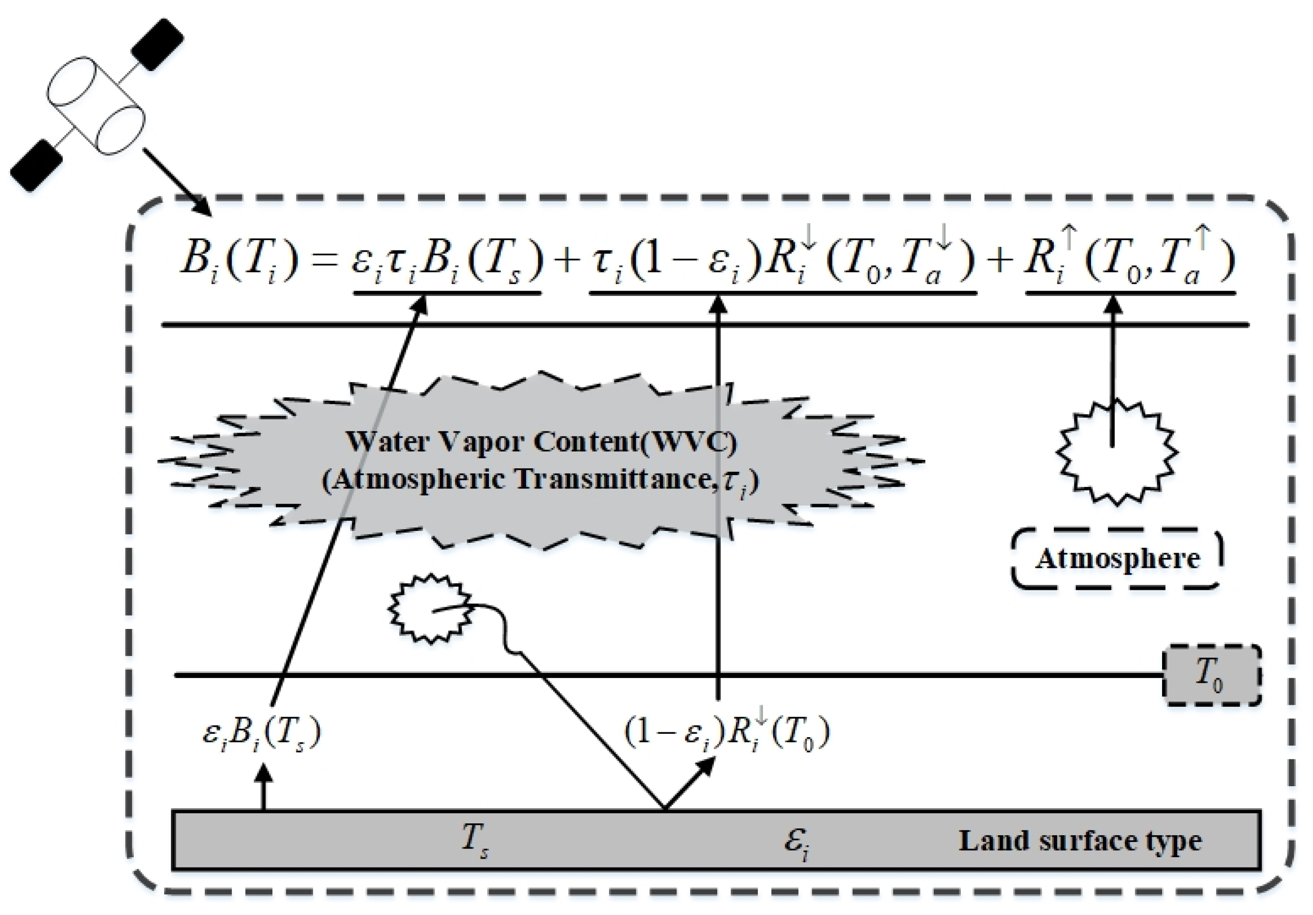
The physical method for NSAT is established based on the thermal radiance of the ground and its transfer from the ground and near-surface air to the remote sensor. The radiation transfer process is shown in Figure 3. The theoretical basis for the remote sensing of NSAT is that the near-surface air exchanges energy with the ground surface and atmospheric profile owing to the temperature difference and transmits the radiation through the atmosphere to the sensor. The type of surface influences the surface radiation, resulting in different intensities of energy exchange with the near-surface air. Therefore, the inversion equation must consider the effect of the surface type (LSE). In other words, the LST influences the NSAT, which in turn affects the atmospheric profile temperature. Surface and near-surface energy is absorbed by the atmosphere, especially, by the water vapor, as it travels through the atmosphere to the sensor [40]. The spectral distribution of radiation emitted from the ground and near the surface depends on the wavelength. The simplified radiation energy balance equation is presented as Equation (1).
B i ( T i ) = ε i τ i B i ( T s ) + τ i ( 1 ε i ) R i ( T 0 , T a ) + R i ( T 0 , T a )
where B i ( T i ) is the thermal radiance received by the sensor in band i;   T i is the satellite BT; ε i is the LSE for band i; τ i is the atmospheric transmittance of band i; B i ( T s ) is the radiance emitted by the surface; T s is the LST; R i ( T 0 , T a ) and R i ( T 0 , T a ) represent the downwelling and upwelling atmospheric radiation of band i, respectively; T 0 is the NSAT; and T a , and T a denote the downwelling and upwelling effective mean temperature of the atmosphere, respectively.
The atmospheric upwelling radiation R i ( T 0 , T a ) can be expressed as in Equation (2) [41,42]:
R i ( T 0 , T a ) = 0 H B ( T h ) τ i ( h , H ) h d h
where T h is the atmospheric temperature at elevation h, H is the sensor height, and τ i ( h , H ) is the atmospheric upwelling transmittance between elevations h and H. Equation (3) can be obtained by solving Equation (2) using the mean value theorem [41,42].
R i ( T 0 , T a ) = ( 1 τ i ) B i ( T 0 , T a )
The atmospheric downwelling radiation R i ( T 0 , T a ) can be considered an integral of the atmospheric radiation from a hemispherical direction and can be expressed as in Equation (4) [41,42].
R i ( T 0 , T a ) = 2 0 π / 2 0 B i ( T h ) τ i ( θ , h , 0 ) h c o s θ s i n θ d h d θ
where θ is the direction angle of the atmospheric downwelling radiation, represents the elevation of the top of the Earth’s atmosphere (km), and τ i ( θ , h , 0 ) represents the atmospheric downwelling transmittance from elevation z to the surface. According to Franc and Cracknell (1994) [41], in clear sky conditions, the upwelling and downwelling transmittances can be considered equal for each thin layer of the atmosphere, i.e., τ i ( θ , h , 0 ) = τ i ( h , H ) . Equation (5) can be obtained using the mean value theorem of integrals:
R i ( T 0 , T a ) = 2 0 π / 2 ( 1 τ i ) B i ( T 0 , T a ) c o s θ s i n θ d θ
Therefore, the atmospheric downwelling radiation can be defined as in Equation (6).
R i ( T 0 , T a ) = ( 1 τ i ) B i ( T 0 , T a )
The substitution of Equations (3) and (6) into Equation (1) yields Equation (7)
B i ( T i ) = ε i τ i B i ( T s ) + τ i ( 1 ε i ) ( 1 τ i ) B i ( T 0 , T a ) + ( 1 τ i ) B i ( T 0 , T a )
Here, T a and T a represent the average atmospheric temperatures. Qin et al. (2001) analyzed these two variables and noted no substantial difference in the solution when the two variables were combined to generate one variable.
B i ( T i ) = ε i τ i B i ( T s ) + ( 1 τ i ) [ 1 + τ i ( 1 ε i ) ] B i ( T 0 , T a )
The key contribution of atmospheric radiation pertains to the bottom layer of the atmosphere [43]. According to the derivation analysis, a nearly linear relationship (Equation (9)) exists between the NSAT and average temperature of the atmosphere in the given conditions [42]. According to the reciprocity theory, a similar relationship exists between the NSAT and satellite BT (Equation (10)) [44].
T a = A 1 T 0 + B 1
T 0 = A 2 T i + B 2
where A 1 and   A 2 are coefficients, B 1 and B 2 are constants, and T i is the satellite BT for band i. The coefficients in Equations (9) and (10) vary across regions and seasons. Therefore, one variable ( T 0 ) can be substituted for the other (Ta) to decrease the unknowns in Equation (8). This analysis shows that although a certain constraint relationship exists between the different temperature variables in the energy balance equation, this relationship cannot be strictly determined, which introduces uncertainties in the calculation process of traditional methods.
The LSE represents the magnitude of radiant energy absorbed and emitted by the ground surface, which is related to the surface type, surface roughness, and water content. The measured values vary with the wavelength and viewing angle. In general, the spectral curve is unique for each surface type, and thus, if the surface type of a pixel is known, the LSE for each band can be obtained. Therefore, it is reasonable to assume that the LSE for all bands can be reduced to an unknown parameter with respect to the surface type, as shown in Equation (11).
ε i = f ( s u r f a c e _ t y p e )
The atmospheric transmittance ( τ i ) in the energy balance equation (Equation (8)) is affected by the atmospheric water vapor and other gases. In general, the WVC undergoes significant fluctuations, whereas the content of other gases (O) remains relatively stable. Therefore, only the atmospheric WVC needs to be determined to obtain the transmittance at different wavelengths. As shown in Equation (12), the transmittance of different wavelength bands can be summarized as a function of the atmospheric WVC.
τ i = f ( W V C , O )
Equation (10) contains four unknowns (LST, NSAT, atmospheric WVC, and surface type). If the physical method is used to invert the NSAT, at least four thermal infrared bands are needed to construct four radiative transfer equations. According to the simulation analysis, the thermal radiation energy emitted by the surface accounts for 75% of the energy received by the sensor when the atmospheric transmittance is higher than 0.65. Consequently, the NSAT inversion algorithm that directly uses the thermal infrared band is not adequately accurate, and thermal infrared remote sensing is more suitable for retrieving the surface temperature. To enhance the accuracy and versatility of the NSAT inversion algorithm, we first invert the LST and LSE and then use the LST and LSE as prior knowledge to further invert the NSAT. Equation (8) indicates that if the atmospheric WVC is known, the NSAT can be retrieved using the three thermal infrared bands. Additionally, if the surface temperature and atmospheric WVC are known, the NSAT can be retrieved using the two thermal infrared bands. The MODTRAN model can obtain as many solutions of equations as possible by setting the variation ranges of parameters such as the surface temperature, air temperature, and atmospheric state under clear sky conditions. The solutions of physical and statistical methods constitute the training and test data for DL, and DL optimization can then be performed to solve the inversion equations.

3.3. Statistical Method

The statistical method for retrieving the NSAT based on thermal infrared remote sensing mainly involves the direct statistical regression of the NSAT and multiple thermal infrared bands [13]. Another statistical algorithm directly uses the NSAT and surface temperature retrieved from thermal infrared remote sensing to perform statistical regression [14,22]. In these methods, the inversion accuracy of a single surface type is reliable over a short period. However, these methods are not portable or versatile over a long period because the influence of other factors such as the LSE on the NSAT is not considered. To eliminate the shortcomings of traditional methods, we use the LST and LSE as prior knowledge. The consideration of these parameters can help eliminate the instability of thermal infrared remote sensing-based NSAT inversion, enhance the computational accuracy, and improve the generality of the algorithm. According to the derivation of the physical method, if the LST and LSE are not used as prior knowledge, the statistical method needs at least four thermal infrared bands to achieve a high accuracy. Because the signal between the different bands is nonlinear, the statistical method can be expressed as in Equation (13).
T 0 = f 1 ( T 1 ) + f 2 ( T 2 ) + + f i ( T i )
where Ti represents the satellite BT of the thermal infrared band i (i ≥ 4), and fi stands for fuzzy statistical function. Here we do not need specific calculation, just need to directly use multisource data to obtain the solutions of the statistical method. For consistency, the location and number of bands used in the statistical and physical methods are identical in this study. Most physical methods do not describe all situations, and statistical methods can thus be an effective complement. From a big data perspective, if the data collected through statistical methods can effectively represent all spatial solutions, then inversion can be achieved through DL. To enhance the inversion accuracy and generality of the algorithm, we collect high-precision statistical sample data from multiple sources.

3.4. DL

In recent years, DL has been widely used in many fields and received considerable attention from the remote sensing community. However, DL techniques are typically regarded as a black box, and the physical mechanism remains to be clarified [23,45,46,47]. As discussed in Section 3.1, DL can be used to couple physical and statistical algorithms. Moreover, Section 3.2 and Section 3.3 describe the sufficient conditions for physical and statistical methods to optimize calculations with DL techniques, which can render the use of DL physically meaningful. Many researchers have presented the principles and technical details associated with the use of DL in the inversion of geophysical parameters and the surface temperature [48,49]. As shown in Figure 4, a fully connected DL-NN consists of an input layer, an output layer, and multiple hidden layers, and the number of neurons in each layer depends on the setting of the initial parameters. The weight and bias of a single neuron are   ( w · X + σ ) , which is activated by the nonlinear function sigmoid function. The result of the activation is the input of the next neuron or output of the entire network. The input of the neuron can be the actual input X of the entire network or the output of the previous neuron.
In the training process, the Kalman filter algorithm is used to enhance the convergence speed of the learning phase and separation ability for highly nonlinear problems. The initial neural network weights are set to be small random numbers (−1, 1). The Kalman filtering process is a recursive mean square estimation process, and the NN weight for each update is calculated based on the previous estimation results and new input data. Consequently, the weights connected to each output node can be updated independently. To rapidly obtain the required root-mean-square error (RMSE), the DL requires only a few iterations, and the results obtained by the NN are highly stable [12,44].

3.5. Model Construction

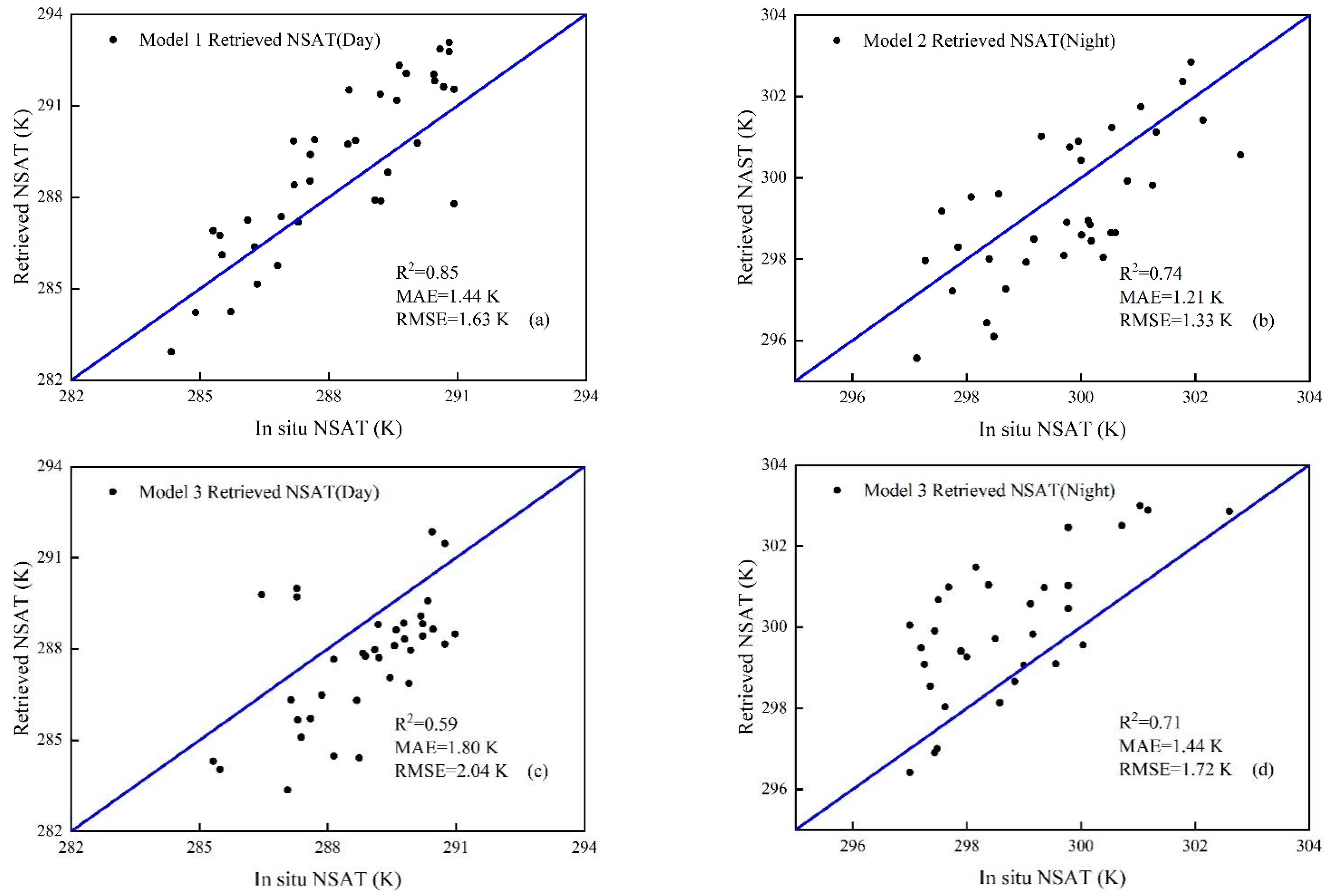
MODIS consists of multiple mid-infrared and thermal infrared bands. MODIS bands 20, 22, and 23 range from 3.5 to 7.2 µm, and bands 29, 30, 31, 32, and 33 range from 8 to 13.5 µm. The mid-infrared band (3.5–4.2 μm) is affected by solar radiation, and its use is therefore mainly suitable for night retrieval, whereas the thermal infrared bands (8–13.5 μm) are suitable for both day and night retrieval. According to the position of the central wavelength and characteristics of the MODIS bands, we constructed three combinatorial modes (Table 2): (1) combinations suitable for day retrievals: LST, LSE, and BT in thermal infrared bands 29, 31, and 32 and WVC (2/5/17/18/19); (2) combinations suitable for night retrievals: LST, LSE, and BT in thermal infrared bands 29, 31, and 32 and infrared bands 20, 22, and 23; and (3) combinations suitable for day and night retrievals: LST, LSE, and BT in thermal infrared bands 29, 31, 32, and 33. Through the trial and error, we set the number of hidden nodes and hidden layers from small to large, and obtained the relatively optimal results. Some of the results are shown in Table 3, Table 4 and Table 5. The first row of the table represents the number of hidden nodes, and the second row represents the accuracy, and the first column represents the number of hidden layers.

4. Results and Validation

4.1. Theoretical Accuracy Validation and Analysis

Simulation data and DL are used to optimize the computational solution process for the physical method. The MODIS sensor provides the water vapor inversion calculation bands (2, 5, 17, 18, and 19). First, we calculate the atmospheric water vapor content [50] and retrieve LST and LSE using the corresponding combination model, which are consistent with those in Table 2 and can be referred to in References [48,49]. Then, we take LST and LSE as prior knowledge, and use the corresponding model combination to continue to retrieve NSAT. The combination 1–3 of inversion of LST and LSE corresponds to model 1–3 in Table 2, and the difference is that the surface temperature and emissivity are unknown. Combination 1 is suitable for day retrieval, and Table 3 summarizes the LST retrieval errors. The LST is retrieved most accurately when the numbers of hidden layers and hidden nodes are 9 and 600, respectively, corresponding to a mean absolute error (MAE) and RMSE of 0.59 K and 0.93 K, respectively. The corresponding MAEs of LSE29, LSE31, and LSE32 are 0.007, 0.005, and 0.006, and the RMSEs are 0.009, 0.006, and 0.004, respectively. The average errors of the emissivity inversions are lower than 0.01.
Combination 2 is suitable for night retrieval because MODIS bands 20, 22, and 23 have an atmospheric window wavelength of 3–5 µm, which is suitable for night use. Because band 33 is affected by the carbon dioxide level, we select the combination of bands 20, 22, 23, 29, 31, and 32 to decrease the amount of data. Table 4 summarizes the LST retrieval errors of Combination 2. The LST is retrieved most accurately when the numbers of hidden layers and hidden nodes are 7 and 500, respectively, with the MAE and RMSE being 0.43 K and 0.65 K, respectively. The corresponding MAEs of LSE20, LSE22, LSE23, LSE29, LSE31, and LSE32 are 0.013, 0.016, 0.016, 0.005, 0.002, and 0.002, and the RMSEs are 0.020, 0.024, 0.025, 0.007, 0.003, and 0.003, respectively. The inversion errors of LSE20, LSE22, and LSE23 are considerably larger than those of LSE29, LSE31, and LSE32.
Combination 3 is suitable for both day and night. Table 5 summarizes the retrieval errors for the LST. The LST is retrieved most accurately when the numbers of hidden layers and hidden nodes are 5 and 800, respectively, with the MAE and RMSE being 0.87 K and 1.02 K, respectively. The corresponding MAEs of LSE29, LSE31, LSE32, and LSE33 are 0.008, 0.007, 0.005, and 0.004, and the RMSEs are 0.010, 0.007, 0.006, and 0.006, respectively. The inversion errors of LSE29 are considerably larger than those of LSE31 and LSE32. Compared to Combination 1, the overall accuracy of the retrieval result is slightly decreased. A comparison of the differences in the input parameters of the two combinations indicates that the addition of water vapor information can enhance the accuracy of the LST retrieval results.
Figure 5 shows the distribution of LSE inversion errors when the three Combinations are the most accurate. The retrieval accuracies of the different combinations are stable, consistent with those of the LST. The LSE retrieval accuracy of Combination 2 is the highest, followed by Combinations 1 and 3. The average retrieval error of the LSE for all three Combinations is less than 0.01. The LSE inversion accuracy of bands 20, 22, and 23 is inferior to that of bands 29, 31, and 32. The main reason is that LSE20, LSE22, and LSE23 have a larger fluctuation range than in the other bands, which deteriorates the retrieval accuracy. The retrieval accuracy of LSE29 is slightly lower than those of LSE31 and LSE32, and the retrieval errors of LSE31 and LSE32 are approximately equal to and lower than 0.006, respectively. The National Aeronautics and Space Administration (NASA) defines MODIS products as having a high pixel quality when the LSE error is smaller than 0.01. To ensure the accuracy of NSAT inversion, we select only LSE31 and LSE32 as the prior knowledge.
The information obtained by the sensor is mainly associated with the LST. We solve Equation (8) for the NSAT considering the LSE and LST as prior knowledge. The process is similar to the inversion calculation of the LST and LSE described above, but the two parameters are simultaneously used as the input information. Table 6 summarizes the retrieval errors of the NSAT for different models.
Figure 6 shows the distribution of the NSAT inversion errors when the three models are the most accurate. The NSAT retrieval accuracies of the models are high. Model 2 (20, 22, 23, 29, 31, 32, LSE, LST) achieves the highest retrieval accuracy (MAE and RMSE of 0.78 K and 0.89 K, respectively), followed by Models 1 (29, 31, 32, WVC, LSE, LST) and 3 (29, 31, 32, 33, LSE, LST), which have MAE and RMSE values of 0.89 K and 1.13 K, respectively, and 1.01 K and 1.26 K, respectively. A comparison of Models 1 and 3 shows that the NSAT retrieval accuracy can be improved by replacing band 33 with the water vapor band information. The retrieval accuracy is different for different band combinations, and the optimal combination must be selected considering the band settings of thermal infrared instruments in specific applications.

4.2. Practical Validation and Analysis

The simulated data mainly represent the solutions of physical methods. To make the inversion more representative, we supplement the high-precision solutions of the corresponding statistical methods. Section 2.2 and Section 3.3 describe the methods to obtain the solutions of the statistical method. The inversion calculation and accuracy after the simulation data are supplemented with statistical data are similar to those of the analysis presented in Section 4.1 and are thus not repeated. Overall, the previous sections describe the NSAT inversion method in which the LST and LSE are used as prior knowledge and DL is coupled with physical and statistical methods.
The study area in this analysis is the North China Plain region (Figure 7), which is one of the three major plains in China and ranges from 32°–40° N and 114°–121° E. The area is a typical alluvial plain with a flat terrain that facilitates transportation, and it contains many rivers and lakes. The North China Plain is a developed agricultural region in China and experiences a temperate monsoon climate. Many ground observations regarding this area are available, which is conducive to analyzing the inversion results.
Two MODIS images are used to demonstrate the PS-DL inversion application. The dates of the Terra/MODIS and Aquia/MODIS images are 14 October 2014 and 1 August 2018 (nighttime), respectively. Mid-infrared data (bands 20, 22, and 23), thermal infrared data (bands 29, 31, 32, and 33), and WVC data (obtained by bands 2, 5, 17, 18, and 19 retrieval) are used as the input parameters for the PS-DL. The inversion process of the surface temperature and emissivity has been described by Mao et al. (2007) and Wang et al. (2021). In this study, the NSAT inversion results are presented.
Figure 8 and Figure 9 show that the overall distribution of the NSAT retrieved by the PS-DL method is similar to the distribution pertaining to the ERA5-Land products. In addition, Figure 10 and Figure 11 show that the differences between the ERA5-Land products and NSAT retrieved by the PS-DL method range from −2 K to 2 K. As shown in Figure 8, the differences in the NSAT retrieval results and ERA5-Land products are significant in certain regions that are mainly agricultural production areas. These differences can be explained by the following aspects: Straw burning occurs after the autumn harvest in the North China Plain in October, and the LSE varies, which influences the NSAT retrieval results. The MAE and RMSE for Models 1 and 3 are 1.18 K and 1.52 K, respectively, and 1.61 K and 1.90 K, respectively. A comparison of the two inversion modes shows that replacing the band 33 information with water vapor information allows the DL to capture more information and improve the retrieval accuracy. As shown in Figure 10 and Figure 11, the NSAT retrieved by Model 2 is the closest to the ERA5-Land products, with the MAE and RMSE being 0.89 K and 1.18 K, respectively. The NSAT retrieval accuracy of Model 3 is slightly worse (MAE and RMSE of 1.33 K and 1.65 K, respectively). The use of more band information helps increase the inversion accuracy. In practical applications, the appropriate combination must be selected according to the specific thermal infrared sensor.
To further evaluate the accuracy of the PS-DL method, the retrieved NSAT is cross-validated against the China Meteorological Forcing Dataset (CMFD). The temporal resolution of this dataset is 3 h, and we evaluate the model accuracy by interpolating the CMFD products with the MODIS imaging time as the base. Figure 12, Figure 13, Figure 14 and Figure 15 show the comparison of the inversion results. In the daytime and nighttime scenarios, Model 1 (MAE and RMSE of 1.46 K and 1.91 K, respectively) and Model 2 (MAE and RMSE of 1.00 K and 1.29 K, respectively) exhibit the highest retrieval accuracies, respectively. Most of the retrieval errors are concentrated between −2 K and 2 K. The cross-validation accuracy with the CMFD product is slightly lower than that of the ERA5-Land product, attributable to the temporal resolution (3 h) for CMFD products. In certain regions, the use of linear interpolation may lead to increased errors. The cross-validation results demonstrate the potential of the PS-DL method in retrieving the NSAT. The inversion error at the junction of water and land is large, attributable to the presence of mixed pixels. Additionally, the energy exchange at the junction of water and land is different from that in the other locations. Therefore, the training data for these regions must be supplemented.
Moreover, we verify the PS-DL performance against ground measured data. The ground verification data are based on ground meteorological observation points in a flat terrain with a single surface type. In situ data acquired in clear sky conditions are compared with the NSAT inversions from Models 1–3. As shown in Figure 16, the MAE and RMSE are, respectively, 1.44 K and 1.63 K for Model 1 and 1.21 K and 1.33 K for Model 2. In the case of Model 3, the inversion accuracy for the nighttime is higher than that for the daytime.

5. Discussion and Conclusions

5.1. Discussion

The NSAT is affected by not only the surface radiation but also the airflow and other factors. Most of the existing methods consider the effect of only the surface temperature or atmospheric profile temperature, which limits their accuracy and portability. In this study, to accurately invert the NSAT, we establish the physical method by considering not only the influence of the LST and LSE but also the relationship between the atmospheric profile temperature (average effective temperature of the atmosphere), satellite BT, and NSAT. Our statistical approach is based on the derivation of the physical method. The main difference is that the NSAT and satellite BT data obtained directly from multiple sources are used as a supplement to the physical method. DL is incorporated to combine physical and statistical methods and exploit the advantages of the three methods.
The inversion of the NSAT using the PS-DL approach yields satisfactory results when the LST and LSE are used as prior knowledge. To demonstrate the importance of using these parameters as prior knowledge, we analyze the inversion accuracy of the NSAT without using the LST and LSE. Five groups of comparative analyses are performed, and the results are shown in Table 7. In Test 3, in which there are only four bands of information, the MAE and RMSE are 1.61 K and 1.90, respectively. The accuracy is enhanced when band 33 is replaced with the water vapor information (Test 1), with the MAE and RMSE being 1.32 K and 1.65 K, respectively. In Test 2, more band information is added, and the accuracy is further enhanced, with the MAE and RMSE being 0.98 K and 1.21 K, respectively. This finding highlights that in given conditions, the accuracy can be increased by increasing the number of bands. A comparison of the values presented in Table 6 and Table 7 indicates that the NSAT inversion accuracy can be increased by using LST and LSE as prior knowledge.
The accuracy of Test 4 (bands 29, 31, 32, LST, LSE), with the MAE and RMSE being 1.11 K and 1.40 K, respectively, is lower than that of Model 1. This finding demonstrates the importance of using the water vapor information for NSAT retrieval. A comparison of Models 2 and 3 shows that increasing the band information can enhance the inversion accuracy. Notably, in practical applications, several satellites may not have adequate thermal bands to complete the inversion. Therefore, we designed Test 5 (bands 31, 32, LST, and LSE), which achieves satisfactory MAE and RMSE values of 1.24 K and 1.56 K, respectively. This analysis demonstrates that the optimal combination must be selected considering the sensor band settings to enhance the NSAT inversion accuracy.

5.2. Conclusions

Considering the advantages and disadvantages of traditional methods, we develop a novel fully coupled framework to robustly invert the NSAT. The proposed PS-DL framework inherits the advantages of physical, statistical, and DL methods. Through the iterative optimization of physical and statistical methods, DL effectively solves the ill-conditioned problem of NSAT inversion and enhances the NSAT inversion accuracy. In this framework, LST and LSE are retrieved first, and then LST and LSE are used as prior knowledge to further retrieve NSAT. This model will become a paradigm for retrieving near-surface air temperature from thermal infrared remote sensing, and the DL for NSAT inversion is not only physically meaningful but also interpretable, which is a milestone in the history of near-surface air temperature retrieval. Because it realizes the coordinated development, mutual promotion, and integration of different methods, the proposed framework demonstrates significant application potential in the inversion of geophysical parameters.
To enhance the accuracy and the portability of the algorithm, the LST and LSE are used as prior knowledge. The best band combinations for NSAT retrieval from MODIS data are bands 20, 22, 23, 29, 31, and 32 with LST and LSE because the influence of the solar radiation is eliminated (nighttime conditions), and the relationship between the ground and atmosphere gradually reaches a state of equilibrium. Consequently, in these conditions, the NSAT experiences low interference and is stable. The inversion accuracy for the combination of bands suitable for day inversion can be enhanced by adding the atmospheric WVC information. The inversion results of different models show that the PS-DL method exhibits a high inversion accuracy in all periods, which satisfies practical application requirements. To further enhance the inversion accuracy, the observation angles can be divided into different intervals to build training and test databases to retrain the DL-NN. The division can also be performed according to different seasons and regions.

Author Contributions

Methodology, software, validation, formal analysis, investigation, data curation, writing—original draft and writing, B.D.; conceptualization, methodology, software, validation, formal analysis, investigation, data curation, writing—original draft, writing—review, editing, project administration and funding acquisition, K.M.; formal analysis, investigation and data curation, S.M.B. and F.M.; resource, formal analysis, investigation and editing, X.-M.W., Z.G., C.J. and G.D. All authors have read and agreed to the published version of the manuscript.

Funding

This project is funded under the Funding by Fengyun Application Pioneering Project (grant no. FY-APP-2022.0205), the National Key R&D Programof China (grant no. 2021YFD1500101), Ningxia Science and Technology Department Flexible Introduction talent project (grant no. 2021RXTDLX14), the Fundamental Research Funds for Central Nonprofit Scientific Institution (grant no. 1610132020014) and the Open Fund of the State Key Laboratory of Remote Sensing Science (grant no. OFSLRSS202201), and the Framework Project of Asia-Pacific Space Cooperation Organization (APSCO) member states (global and key regional drought forecasting and monitoring, grant no. 20222144).

Data Availability Statement

Data openly available in a public repository.

Acknowledgments

The authors thank the China Meteorological Administration for providing ground-based measurements, the NASA Earth Observation System Data and Information System for providing MODIS data, the Institute of Qinghai–Tibetan Plateau of the Chinese Academy of Sciences for providing the CMFD dataset, and the ECMWF for providing climate reanalysis data.

Conflicts of Interest

The authors declare that they have no known competing financial interests or personal relationships that could have appeared to influence the work reported in this paper.

References

  1. Huang, Y.; Chen, Z.; Yu, T.; Huang, X.; Gu, X. Agricultural remote sensing big data: Management and applications. J. Integr. Agric. 2018, 17, 1915–1931. [Google Scholar] [CrossRef]
  2. Kolokotroni, M.; Giridharan, R. Urban heat island intensity in London: An investigation of the impact of physical characteristics on changes in outdoor air temperature during summer. Sol. Energy 2008, 82, 986–998. [Google Scholar] [CrossRef] [Green Version]
  3. Nieto, H.; Sandholt, I.; Aguado, I.; Chuvieco, E.; Stisen, S. Air temperature estimation with MSG-SEVIRI data: Calibration and validation of the TVX algorithm for the Iberian Peninsula. Remote Sens. Environ. 2011, 115, 107–116. [Google Scholar] [CrossRef] [Green Version]
  4. Saaroni, H.; Ziv, B. Estimating the Urban Heat Island Contribution to Urban and Rural Air Temperature Differences over Complex Terrain: Application to an Arid City. J. Appl. Meteorol. Climatol. 2010, 49, 2159–2166. [Google Scholar] [CrossRef]
  5. Zaksek, K.; Schroedter-Homscheidt, M. Air temperature in high temporal and spatial resolution from a combination of the SEVIRI and MODIS instruments. In Proceedings of the EUMETSAT Meteorological Satellite Conference, Darmstadt, Germany, 8–12 September 2008; pp. 1–8. [Google Scholar]
  6. Chen, S.; Yang, Y.; Deng, F.; Zhang, Y.; Liu, D.; Liu, C.; Gao, Z. A high-resolution monitoring approach of canopy urban heat island using a random forest model and multi-platform observations. Atmos. Meas. Tech. 2022, 15, 735–756. [Google Scholar] [CrossRef]
  7. Yang, Y.; Zhang, M.; Li, Q.; Chen, B.; Gao, Z.; Ning, G.; Liu, C.; Li, Y.; Luo, M. Modulations of surface thermal environment and agricultural activity on intraseasonal variations of summer diurnal temperature range in the Yangtze River Delta of China. Sci. Total Environ. 2020, 736, 139445. [Google Scholar] [CrossRef] [PubMed]
  8. Yang, Y.; Guo, M.; Ren, G.; Liu, S.; Zong, L.; Zhang, Y.; Zheng, Z.; Miao, Y.; Zhang, Y. Modulation of Wintertime Canopy Urban Heat Island (CUHI) Intensity in Beijing by Synoptic Weather Pattern in Planetary Boundary Layer. J. Geophys. Res. Atmos. 2022, 127, e2021JD035988. [Google Scholar] [CrossRef]
  9. Sun, Y.-J.; Wang, J.-F.; Zhang, R.-H.; Gillies, R.R.; Xue, Y.; Bo, Y.-C. Air temperature retrieval from remote sensing data based on thermodynamics. Theor. Appl. Climatol. 2005, 80, 37–48. [Google Scholar] [CrossRef]
  10. Boyer, D.G. Estimation of Daily Temperature Means Using Elevation and Latitude in Mountainous Terrain. JAWRA J. Am. Water Resour. Assoc. 1984, 20, 583–588. [Google Scholar] [CrossRef]
  11. Ishida, T.; Kawashima, S. Use of cokriging to estimate surface air temperature from elevation. Theor. Appl. Climatol. 1993, 47, 147–157. [Google Scholar] [CrossRef]
  12. Mao, K.; Tang, H.J.; Wang, X.F.; Zhou, Q.B.; Wang, D.L. Near-surface air temperature estimation from ASTER data based on neural network algorithm. Int. J. Remote Sens. 2008, 29, 6021–6028. [Google Scholar] [CrossRef]
  13. Cresswell, M.P.; Morse, A.P.; Thomson, M.C.; Connor, S.J. Estimating surface air temperatures, from Meteosat land surface temperatures, using an empirical solar zenith angle model. Int. J. Remote Sens. 1999, 20, 1125–1132. [Google Scholar] [CrossRef]
  14. Shi, Y.; Jiang, Z.; Dong, L.; Shen, S. Statistical estimation of high-resolution surface air temperature from MODIS over the Yangtze River Delta, China. J. Meteorol. Res. 2017, 31, 448–454. [Google Scholar] [CrossRef]
  15. Stisen, S.; Sandholt, I.; Nørgaard, A.; Fensholt, R.; Eklundh, L. Estimation of diurnal air temperature using MSG SEVIRI data in West Africa. Remote Sens. Environ. 2007, 110, 262–274. [Google Scholar] [CrossRef]
  16. Alonso, L.; Renard, F. Integrating Satellite-Derived Data as Spatial Predictors in Multiple Regression Models to Enhance the Knowledge of Air Temperature Patterns. Urban Sci. 2019, 3, 101. [Google Scholar] [CrossRef] [Green Version]
  17. Lin, X.; Zhang, W.; Huang, Y.; Sun, W.; Han, P.; Yu, L.; Sun, F. Empirical Estimation of Near-Surface Air Temperature in China from MODIS LST Data by Considering Physiographic Features. Remote Sens. 2016, 8, 629. [Google Scholar] [CrossRef] [Green Version]
  18. Janatian, N.; Sadeghi, M.; Sanaeinejad, S.H.; Bakhshian, E.; Farid, A.; Hasheminia, S.M.; Ghazanfari, S. A statistical framework for estimating air temperature using MODIS land surface temperature data. Int. J. Climatol. 2017, 37, 1181–1194. [Google Scholar] [CrossRef]
  19. Vancutsem, C.; Ceccato, P.; Dinku, T.; Connor, S.J. Evaluation of MODIS land surface temperature data to estimate air temperature in different ecosystems over Africa. Remote Sens. Environ. 2010, 114, 449–465. [Google Scholar] [CrossRef]
  20. Xu, Y.; Qin, Z.; Shen, Y. Estimation of near surface air temperature from MODIS data in the Yangtze River Delta. Trans. Chin. Soc. Agric. Eng. 2011, 27, 63–68. [Google Scholar] [CrossRef]
  21. Zhu, S.; Zhou, C.; Zhang, G.; Zhang, H.; Hua, J. Preliminary verification of instantaneous air temperature estimation for clear sky conditions based on SEBAL. Meteorol. Atmos. Phys. 2017, 129, 71–81. [Google Scholar] [CrossRef]
  22. Mostovoy, G.V.; King, R.L.; Reddy, K.R.; Kakani, V.G.; Filippova, M.G. Statistical Estimation of Daily Maximum and Minimum Air Temperatures from MODIS LST Data over the State of Mississippi. GIScience Remote Sens. 2006, 43, 78–110. [Google Scholar] [CrossRef] [Green Version]
  23. Zhang, R.; Rong, Y.; Tian, J.; Su, H.; Li, Z.-L.; Liu, S. A Remote Sensing Method for Estimating Surface Air Temperature and Surface Vapor Pressure on a Regional Scale. Remote Sens. 2015, 7, 6005–6025. [Google Scholar] [CrossRef] [Green Version]
  24. Jang, J.-D.; Viau, A.A.; Anctil, F. Neural network estimation of air temperatures from AVHRR data. Int. J. Remote Sens. 2004, 25, 4541–4554. [Google Scholar] [CrossRef]
  25. Xu, Y.; Knudby, A.; Shen, Y.; Liu, Y. Mapping Monthly Air Temperature in the Tibetan Plateau from MODIS Data Based on Machine Learning Methods. IEEE J. Sel. Top. Appl. Earth Obs. Remote Sens. 2018, 11, 345–354. [Google Scholar] [CrossRef]
  26. Acharya, P.K.; Berk, A.; Anderson, G.P.; Larsen, N.F.; Tsay, S.C.; Stamnes, K.H. MODTRAN4: Multiple scattering and bi-directional reflectance distribution function (BRDF) upgrades to MODTRAN. Opt. Spectrosc. Tech. Instrum. Atmos. Space Res. III 1999, 3756, 354–362. [Google Scholar] [CrossRef]
  27. Wang, P.; Liu, K.Y.; Cwik, T.; Green, R. MODTRAN on supercomputers and parallel computers. Parallel Comput. 2002, 28, 53–64. [Google Scholar] [CrossRef]
  28. Wan, Z.; Zhang, Y.; Zhang, Q.; Li, Z.-L. Quality Assessment and Validation of the MODIS Global Land Surface Temperature. Int. J. Remote Sens. 2004, 25, 261–274. [Google Scholar] [CrossRef]
  29. Fang, S.; Mao, K.; Xia, X.; Wang, P.; Shi, J.; Bateni, S.M.; Xu, T.; Cao, M.; Heggy, E.; Qin, Z. Dataset of daily near-surface air temperature in China from 1979 to 2018. Earth Syst. Sci. Data 2022, 14, 1413–1432. [Google Scholar] [CrossRef]
  30. Wang, P.; Mao, K.; Meng, F.; Qin, Z.; Fang, S.; Bateni, S.M. A daily highest air temperature estimation method and spatial–temporal changes analysis of high temperature in China from 1979 to 2018. Geosci. Model Dev. 2022, 15, 6059–6083. [Google Scholar] [CrossRef]
  31. Hoffmann, L.; Günther, G.; Li, D.; Stein, O.; Wu, X.; Griessbach, S.; Heng, Y.; Konopka, P.; Müller, R.; Vogel, B.; et al. From ERA-Interim to ERA5: The considerable impact of ECMWF’s next-generation reanalysis on Lagrangian transport simulations. Atmos. Chem. Phys. 2019, 19, 3097–3124. [Google Scholar] [CrossRef]
  32. Urraca, R.; Huld, T.; Gracia-Amillo, A.; Martinez-de-Pison, F.J.; Kaspar, F.; Sanz-Garcia, A. Evaluation of global horizontal irradiance estimates from ERA5 and COSMO-REA6 reanalyses using ground and satellite-based data. Sol. Energy 2018, 164, 339–354. [Google Scholar] [CrossRef]
  33. He, J.; Yang, K.; Tang, W.; Lu, H.; Qin, J.; Chen, Y.; Li, X. The first high-resolution meteorological forcing dataset for land process studies over China. Sci. Data 2020, 7, 25. [Google Scholar] [CrossRef] [PubMed] [Green Version]
  34. Yang, K.; He, J.; Tang, W.; Qin, J.; Cheng, C.C.K. On downward shortwave and longwave radiations over high altitude regions: Observation and modeling in the Tibetan Plateau. Agric. For. Meteorol. 2010, 150, 38–46. [Google Scholar] [CrossRef]
  35. Yang, K.; He, J. China meteorological forcing dataset (1979–2018). Natl. Tibet. Plateau Data Cent. 2019. [Google Scholar] [CrossRef]
  36. LeCun, Y.; Bengio, Y.; Hinton, G. Deep learning. Nature 2015, 521, 436–444. [Google Scholar] [CrossRef] [PubMed]
  37. Yin, H.; Yang, S.; Zhu, X.; Jin, S.; Wang, X. Satellite Fault Diagnosis Using Support Vector Machines Based on a Hybrid Voting Mechanism. Sci. World J. 2014, 2014, 582042. [Google Scholar] [CrossRef] [Green Version]
  38. Mao, K.; Zuo, Z.; Shen, X.; Xu, T.; Gao, C.; Liu, G. Retrieval of Land-surface Temperature from AMSR2 Data Using a Deep Dynamic Learning Neural Network. Chin. Geogr. Sci. 2018, 28, 1–11. [Google Scholar] [CrossRef] [Green Version]
  39. Zhao, B.; Mao, K.; Cai, Y.; Shi, J.; Li, Z.-L.; Qin, Z.; Meng, X.; Shen, X.; Guo, Z. A combined Terra and Aqua MODIS land surface temperature and meteorological station data product for China from 2003 to 2017. Earth Syst. Sci. Data 2020, 12, 2555–2577. [Google Scholar] [CrossRef]
  40. Dozier, J. A method for satellite identification of surface temperature fields of subpixel resolution. Remote Sens. Environ. 1981, 11, 221–229. [Google Scholar] [CrossRef]
  41. Franc, G.B.; Cracknell, A.P. Retrieval of land and sea surface temperature using NOAA-11 AVHRR· data in north-eastern Brazil. Int. J. Remote Sens. 1994, 15, 1695–1712. [Google Scholar] [CrossRef]
  42. Qin, Z.; Karnieli, A.; Berliner, P. A Mono-Window Algorithm for Retrieving Land Surface Temperature from Landsat TM data and its Application to the Israel-Egypt Border Region. Int. J. Remote Sens. 2001, 22, 3719–3746. [Google Scholar] [CrossRef]
  43. Sobrino, J.; Coll, C.; Caselles, V. Atmospheric correction for land surface temperature using NOAA-11 AVHRR channels 4 and 5. Remote Sens. Environ. 1991, 38, 19–34. [Google Scholar] [CrossRef]
  44. Mao, K.; Shi, J.; Li, Z.; Tang, H. An RM-NN algorithm for retrieving land surface temperature and emissivity from EOS/MODIS data. J. Geophys. Res. 2007, 112, 1. [Google Scholar] [CrossRef]
  45. Del Frate, F.; Solimini, D. On neural network algorithms for retrieving forest biomass from SAR data. IEEE Trans. Geosci. Remote Sens. 2004, 42, 24–34. [Google Scholar] [CrossRef] [Green Version]
  46. Shen, H.; Jiang, Y.; Li, T.; Cheng, Q.; Zeng, C.; Zhang, L. Deep learning-based air temperature mapping by fusing remote sensing, station, simulation and socioeconomic data. Remote Sens. Environ. 2020, 240, 111692. [Google Scholar] [CrossRef] [Green Version]
  47. Yuan, Q.; Shen, H.; Li, T.; Li, Z.; Li, S.; Jiang, Y.; Xu, H.; Tan, W.; Yang, Q.; Wang, J.; et al. Deep learning in environmental remote sensing: Achievements and challenges. Remote Sens. Environ. 2020, 241, 111716. [Google Scholar] [CrossRef]
  48. Mao, K.; Shi, J.; Tang, H.; Li, Z.-L.; Wang, X.; Chen, K.-S. A Neural Network Technique for Separating Land Surface Emissivity and Temperature from ASTER Imagery. IEEE Trans. Geosci. Remote Sens. 2007, 46, 200–208. [Google Scholar] [CrossRef]
  49. Wang, H.; Mao, K.; Yuan, Z.; Shi, J.; Cao, M.; Qin, Z.; Duan, S.; Tang, B. A method for land surface temperature retrieval based on model-data-knowledge-driven and deep learning. Remote Sens. Environ. 2021, 265, 112665. [Google Scholar] [CrossRef]
  50. Mao, K.; Qin, Z.; Shi, J.; Gong, P. A Practical Split-window Algorithm for Retrieving Land-surface Temperature from MODIS Data. Int. J. Remote Sens. 2005, 26, 3181–3204. [Google Scholar] [CrossRef]
Figure 1. LSE of (a) soil, (b) vegetation, (c) water, and (d) rock. (A, B, C, D, E and F indicate different subclasses).
Remotesensing 14 05812 g001
Figure 2. Proposed fully coupled physical–statistical–deep learning framework for retrieving near-surface air temperature.
Remotesensing 14 05812 g002
Figure 3. Simplified diagram of the thermal radiation transfer modeling to relate the LST, LSE, and NSAT.
Remotesensing 14 05812 g003
Figure 4. Fully connected layer DL-NN.
Remotesensing 14 05812 g004
Figure 5. Validation of the LSE based on simulation data for Combination 1, 2, and 3.
Remotesensing 14 05812 g005
Figure 6. Validation based on simulation data when Models (a) 1, (b) 2, and (c) 3 have a well-trained DL-NN with the optimal numbers of hidden layers and nodes.
Remotesensing 14 05812 g006
Figure 7. Study area (North China Plain) and location.
Remotesensing 14 05812 g007
Figure 8. (a) ERA5-Land product; NSAT retrieved by (b) Model 1 and (c) Model 3. White areas represent invalid values (14 October 2014; daytime).
Remotesensing 14 05812 g008
Figure 9. (a) ERA5-Land product; NSAT retrieved by (b) Model 2 and (c) Model 3. White areas represent invalid values (1 August 2018; nighttime).
Remotesensing 14 05812 g009
Figure 10. Validation based on the difference (K) between the ERA5-Land NSAT products and NSAT retrieved using the PS-DL method. Difference between (a) Figure 8a,b; (b) Figure 8a,c. White areas represent invalid values.
Remotesensing 14 05812 g010
Figure 11. Validation based on the difference (K) between the ERA5-Land NSAT products and NSAT retrieved using the PS-DL method. Difference between (a) Figure 9a,b; (b) Figure 9a,c. White areas represent invalid values.
Remotesensing 14 05812 g011
Figure 12. CMFD product (14 October 2014; daytime).
Remotesensing 14 05812 g012
Figure 13. Cross-validation. Difference (K) between the CMFD NSAT products and NSAT retrieved using the PS-DL method. Difference between (a) Figure 8b and Figure 12, (b) Figure 8c and Figure 12. White areas represent invalid values.
Remotesensing 14 05812 g013
Figure 14. CMFD product (1 August 2018; nighttime).
Remotesensing 14 05812 g014
Figure 15. Cross-validation. Difference (K) between the CMFD NSAT products and NSAT retrieved using the PS-DL method. Difference between (a) Figure 10b and Figure 14, (b) Figure 10c and Figure 14. White areas represent invalid values.
Remotesensing 14 05812 g015
Figure 16. In situ validation of inversion results of Models 1–3 for different conditions.
Remotesensing 14 05812 g016
Table 1. Overview of the remote sensing and assimilation data datasets used in this study.
VariableDataset(s)Resolution (Spatial/Temporal)Data Source
Brightness temperature (BT)MOD/MYD021KM 1 km/dailyNASA LP DAAC
Land surface temperature (LST)MOD/MYD11A11 km/dailyNASA LP DAAC
Land surface emissivity (LSE)MOD/MYD11A11 km/dailyNASA LP DAAC
Near-surface air temperature (NSAT)ERA5-Land0.1°/hourlyECMWF
CMFD0.1°/3 hTPDC
In situ1 m/hourlyCNMIC
Table 2. Band combinations suitable for the retrieval of near-surface air temperature at different times.
ModelSituationVariables
1DayBTs and LSEs of TIR bands 29/31/32 with WVC and LST
2NightBTs and LSEs of TIR bands 29/31/32 and bands 20/22/23 and LST
3Day and NightBTs and LSEs of TIR bands 29/31/32/33 and LST
Table 3. LST retrieval errors for Combination 1.
H-N400500600700800
H-L MAERMSEMAERMSEMAERMSEMAERMSEMAERMSE
30.711.010.610.930.620.930.610.930.640.96
40.620.930.620.940.611.050.620.960.761.17
50.631.040.600.920.620.940.884.640.711.48
60.641.020.861.650.801.250.633.730.707.49
70.691.730.620.954.0611.490.772.070.621.11
80.600.910.831.690.871.330.661.260.690.96
90.640.970.721.320.590.930.630.990.651.05
100.611.020.620.940.800.960.771.170.691.06
H-L is the hidden layer, H-N is the hidden node.
Table 4. LST retrieval errors for Combination 2.
H-N400500600700800
H-LMAERMSEMAERMSEMAERMSEMAERMSEMAERMSE
30.781.030.831.070.691.010.630.870.50.72
40.580.820.751.560.610.950.610.870.570.84
50.650.910.660.900.640.880.785.510.50.71
60.640.880.760.990.520.750.540.890.784.21
70.731.370.430.650.580.901.559.470.6912.21
80.630.900.550.980.720.980.560.860.660.89
90.620.860.630.950.731.160.591.000.721.35
100.741.030.8311.620.810.860.760.920.630.96
Table 5. LST retrieval errors for Combination 3.
H-N400500600700800
H-L MAERMSEMAERMSEMAERMSEMAERMSEMAERMSE
30.981.120.961.110.911.060.911.050.921.06
40.911.060.981.120.911.060.901.050.921.06
50.961.100.971.130.891.040.901.050.871.02
60.931.310.911.060.901.050.911.170.901.07
70.921.060.941.090.911.080.911.060.891.04
80.961.120.941.100.991.260.871.020.951.12
90.891.100.951.110.911.060.921.150.901.30
100.931.100.951.100.961.120.931.290.921.15
Table 6. (a). NSAT retrieval errors for Model 1. (b). NSAT retrieval errors for Model 2. (c). NSAT retrieval errors for Model 3.
(a)
H-N400500600700800
H-L MAERMSEMAERMSEMAERMSEMAERMSEMAERMSE
30.911.210.951.210.921.250.941.410.961.18
40.921.200.971.220.951.180.951.321.021.21
51.011.190.951.220.971.240.981.211.051.22
60.951.180.961.280.991.280.931.220.951.25
70.981.220.931.241.011.260.991.190.971.27
81.052.370.891.131.051.221.051.240.991.31
90.931.311.011.190.981.230.951.250.991.28
100.941.290.961.190.951.230.971.340.971.27
(b)
H-N400500600700800
H-LMAERMSEMAERMSEMAERMSEMAERMSEMAERMSE
30.821.020.821.040.851.050.821.050.861.03
40.811.010.831.030.861.060.811.060.841.03
50.851.020.841.060.861.070.821.060.831.03
60.851.010.821.040.841.050.780.890.831.04
70.841.080.831.050.881.060.831.070.851.05
80.861.020.941.030.871.070.881.090.861.05
90.911.020.911.010.951.090.821.020.881.06
100.880.990.880.980.811.050.851.040.911.09
(c)
H-N400500600700800
H-L MAERMSEMAERMSEMAERMSEMAERMSEMAERMSE
31.081.281.111.351.081.311.091.291.081.32
41.061.291.081.281.071.341.081.281.091.28
51.111.321.071.271.151.351.081.311.111.32
61.091.311.081.291.051.361.071.281.121.35
71.081.281.111.341.061.321.081.311.081.37
81.061.271.121.321.011.261.061.321.081.31
91.071.311.091.351.071.321.081.271.091.35
101.071.341.081.311.071.351.091.351.061.35
Table 7. Errors associated with test results based on different band combinations.
TestBand CombinationMAERMSE
1BTs of TIR bands 29/31/32 with WVC1.321.65
2BTs of TIR bands 29/31/32 and bands 20/22/230.981.21
3BTs of TIR bands 29/31/32/331.611.90
4BTs of TIR bands 29/31/32 and LST, LSE1.111.40
5BTs of TIR bands 31/32 and LST, LSE1.241.56
Publisher’s Note: MDPI stays neutral with regard to jurisdictional claims in published maps and institutional affiliations.

