

An Automatic Approach to Extracting Large-Scale Three-Dimensional Road Networks Using Open-Source Data

Abstract
:1. Introduction
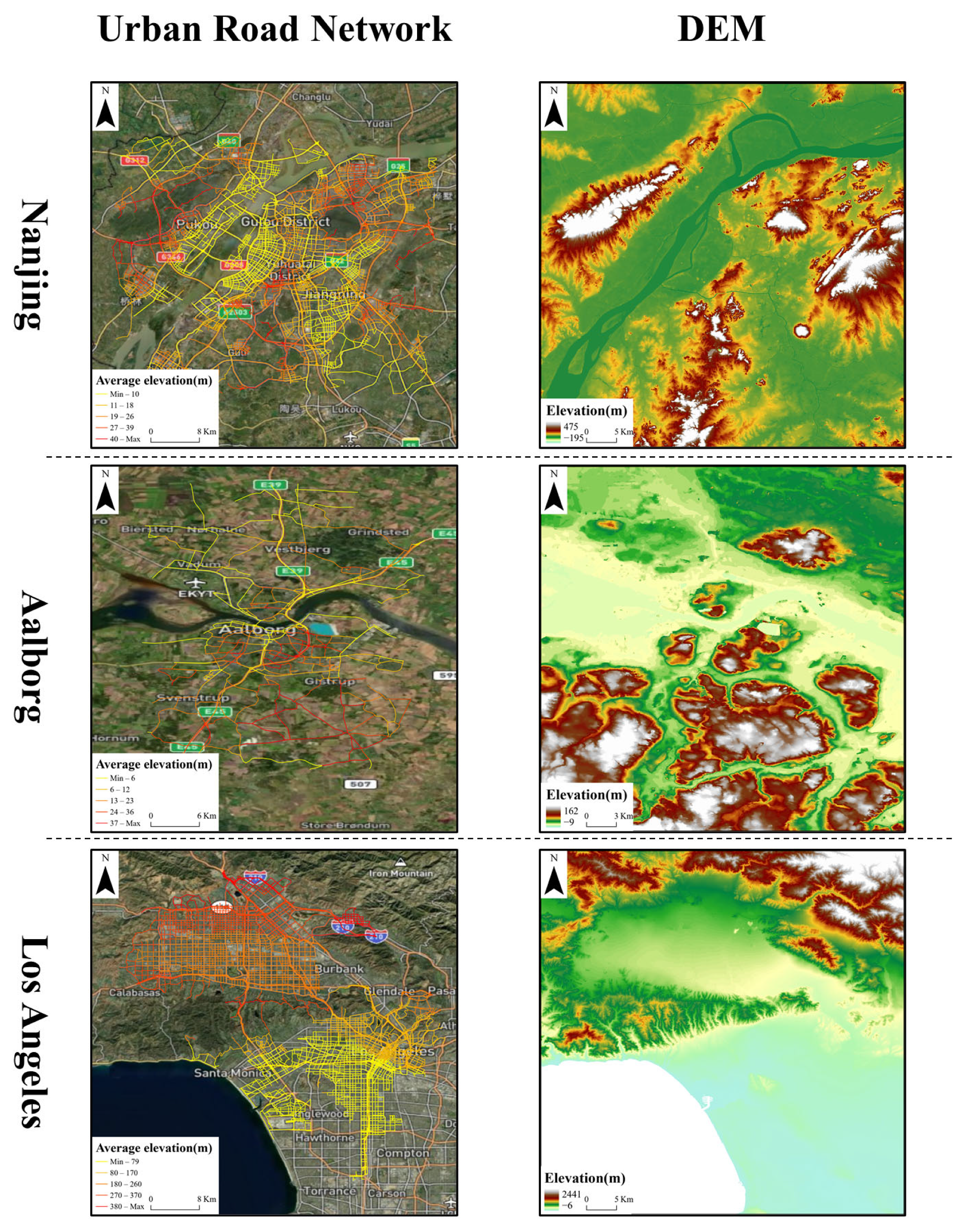
2. Data
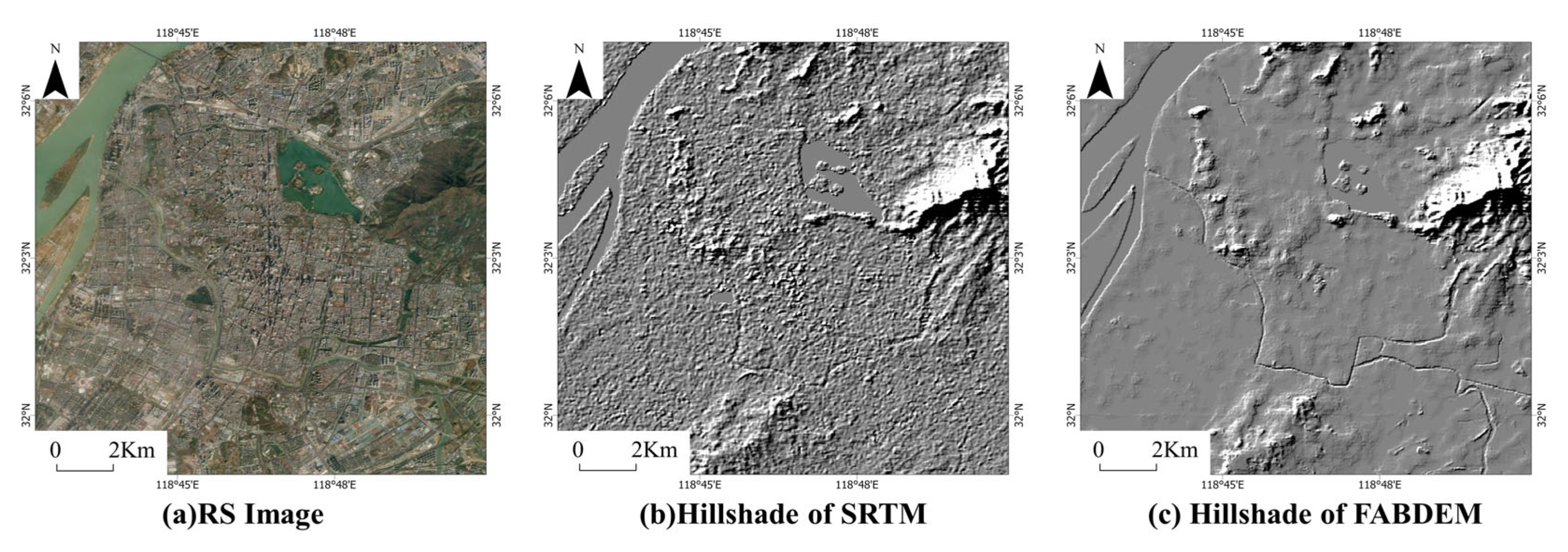
2.1. OSM
2.2. AW3D30 DSM
2.3. FABDEM
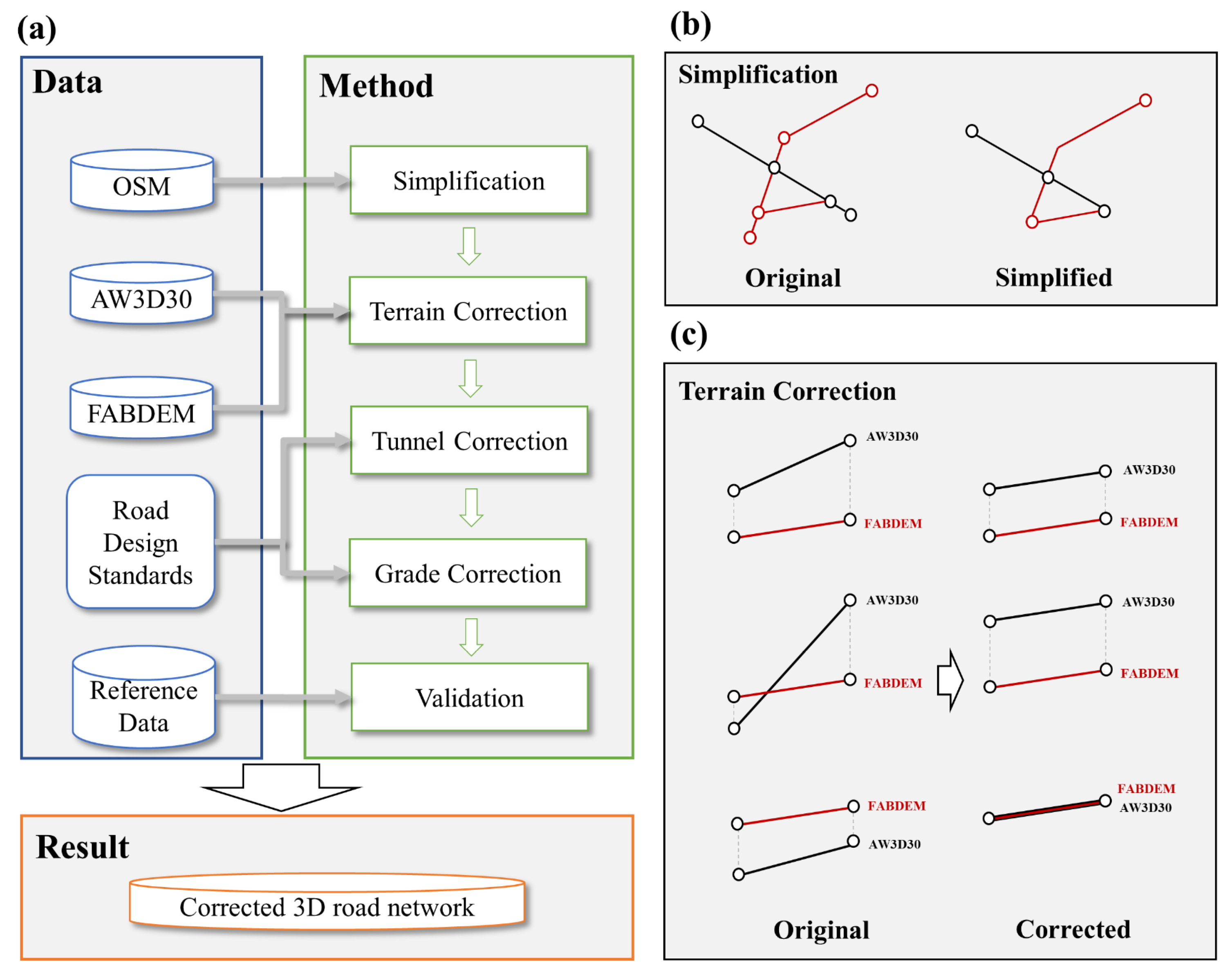
3. Method
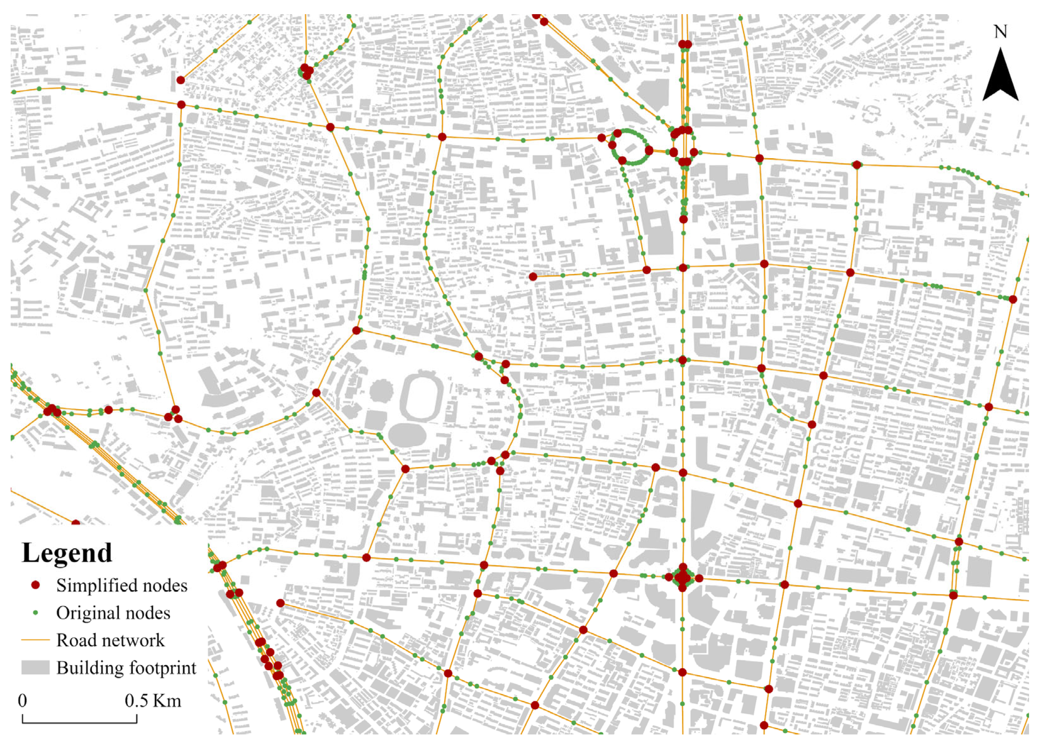
3.1. Simplification
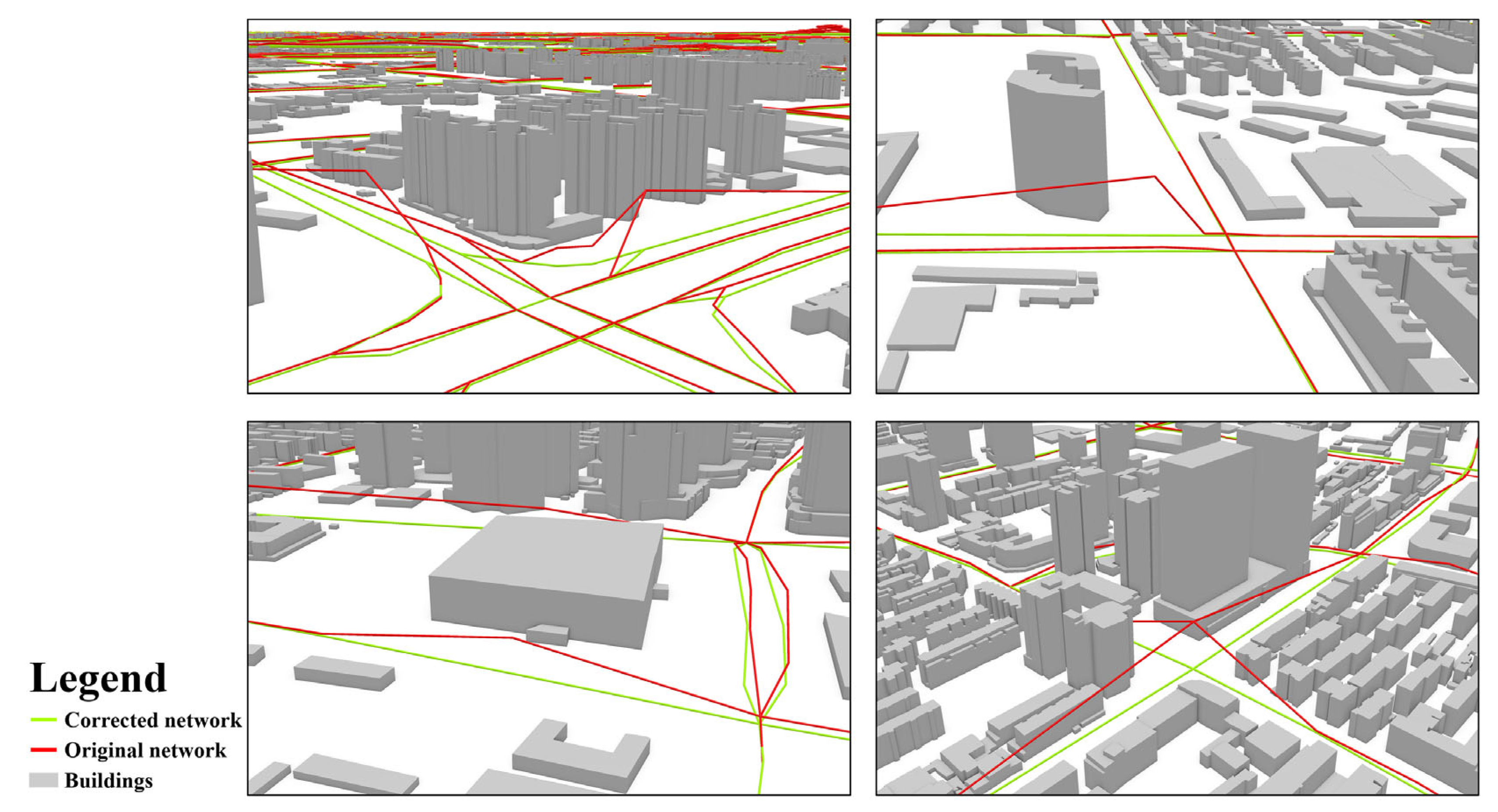
3.2. Correction
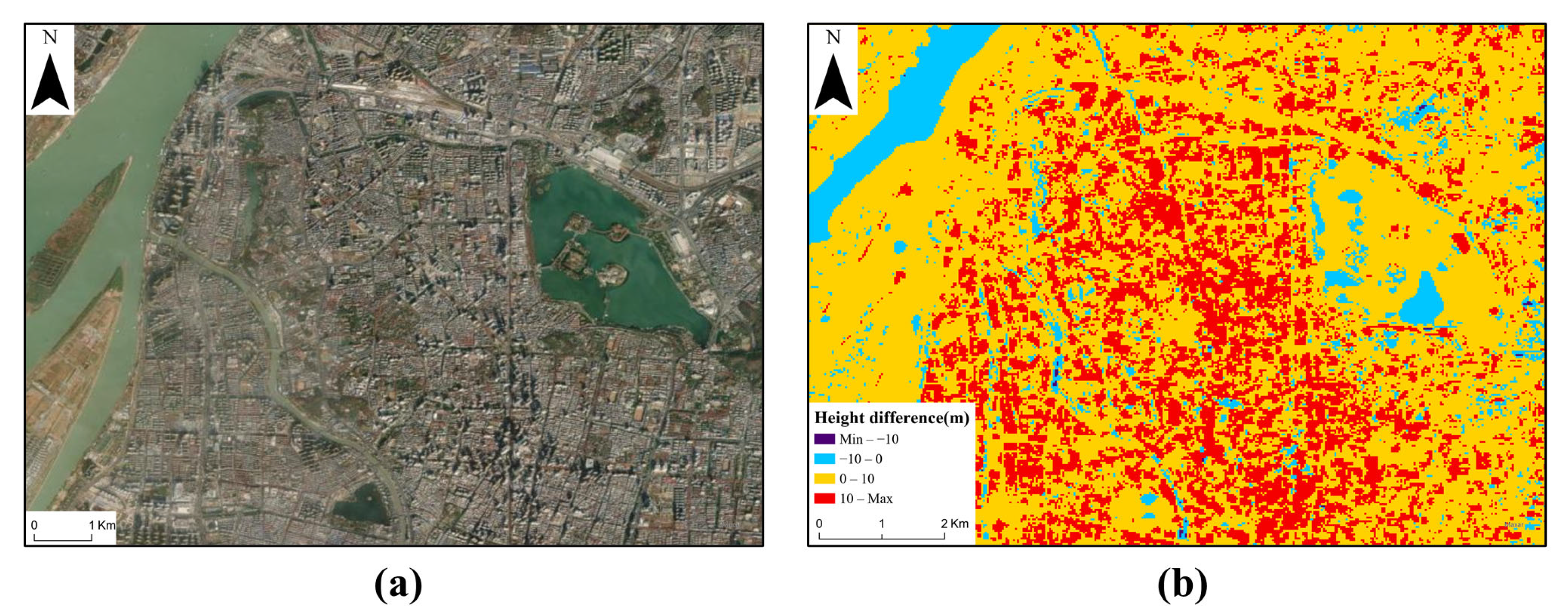
3.2.1. Terrain Correction
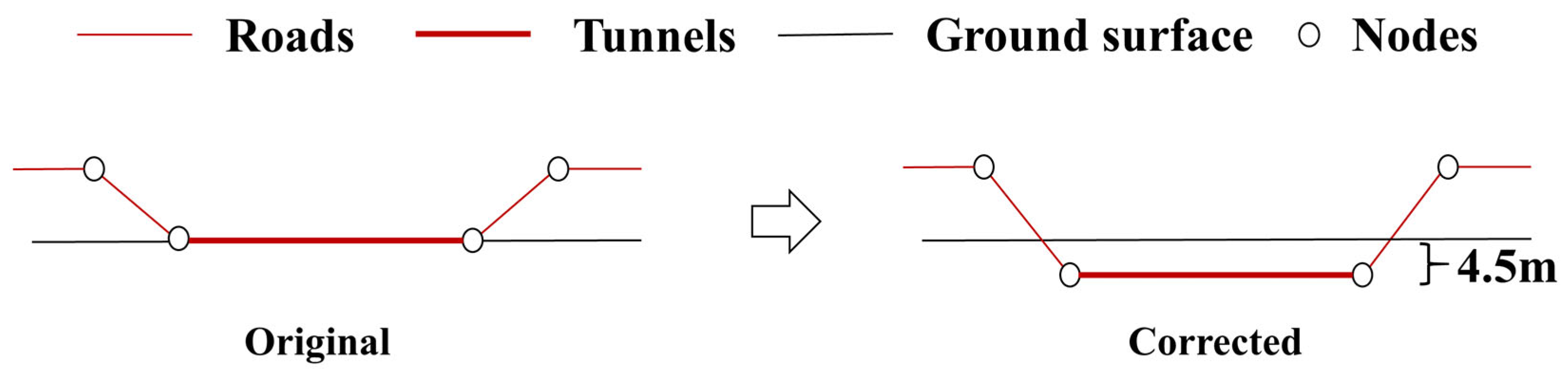
3.2.2. Tunnel Correction
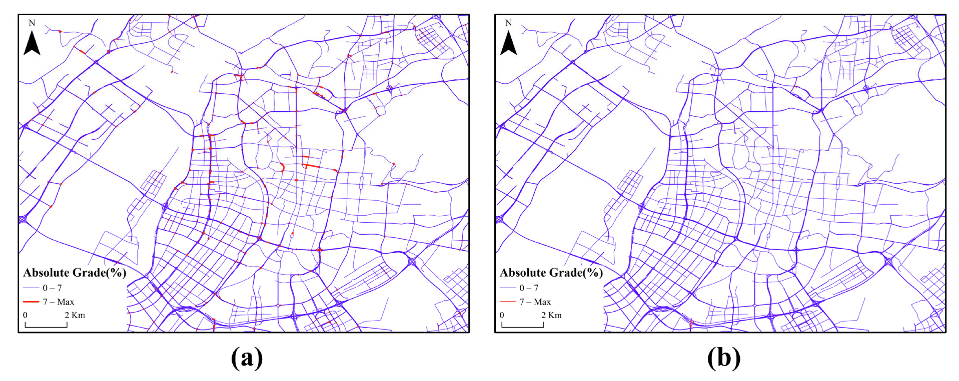
3.2.3. Grade Correction
3.3. Validation with Reference Data
4. Result
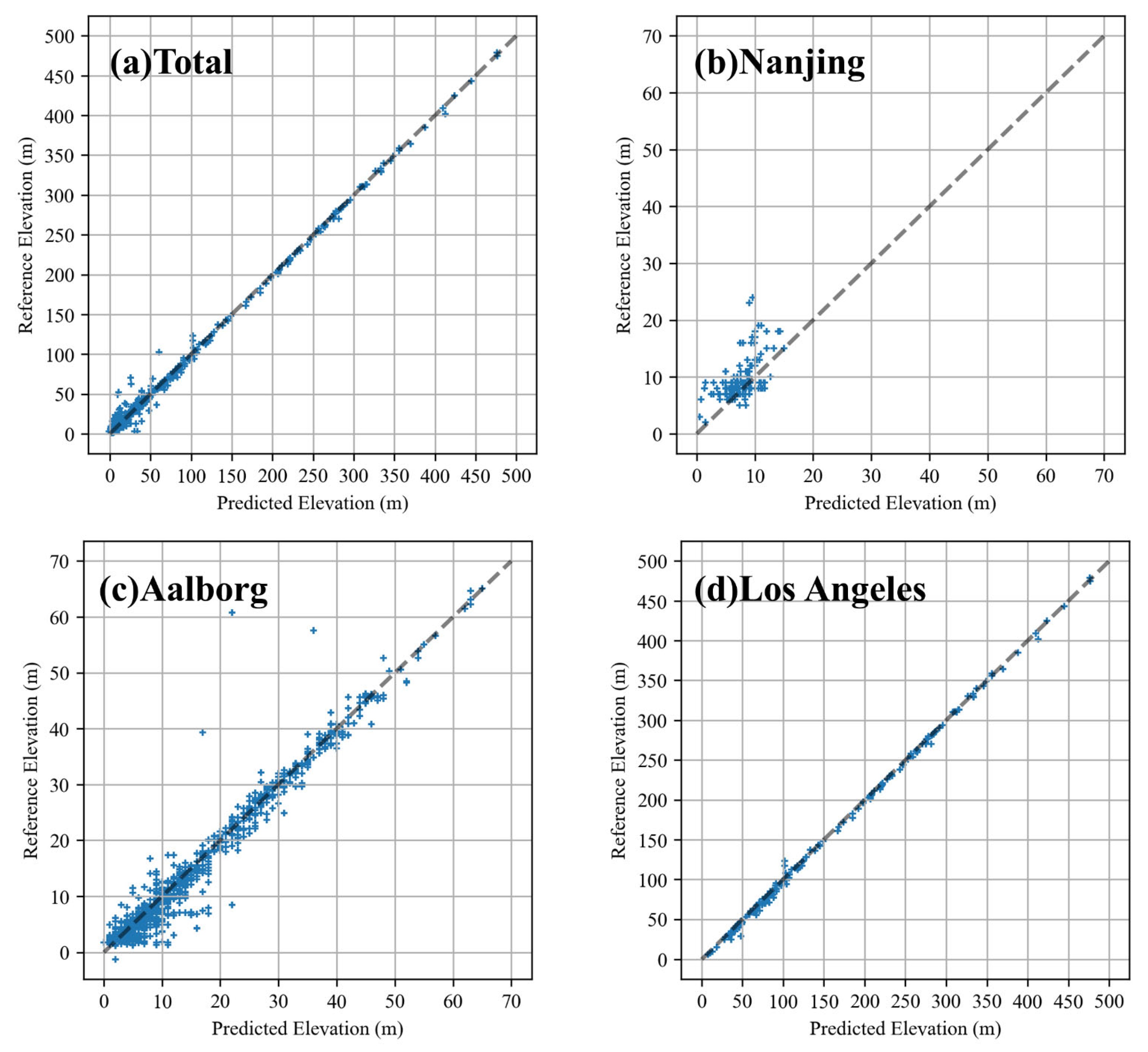
4.1. Accuracy Assessment of Road Network Elevation
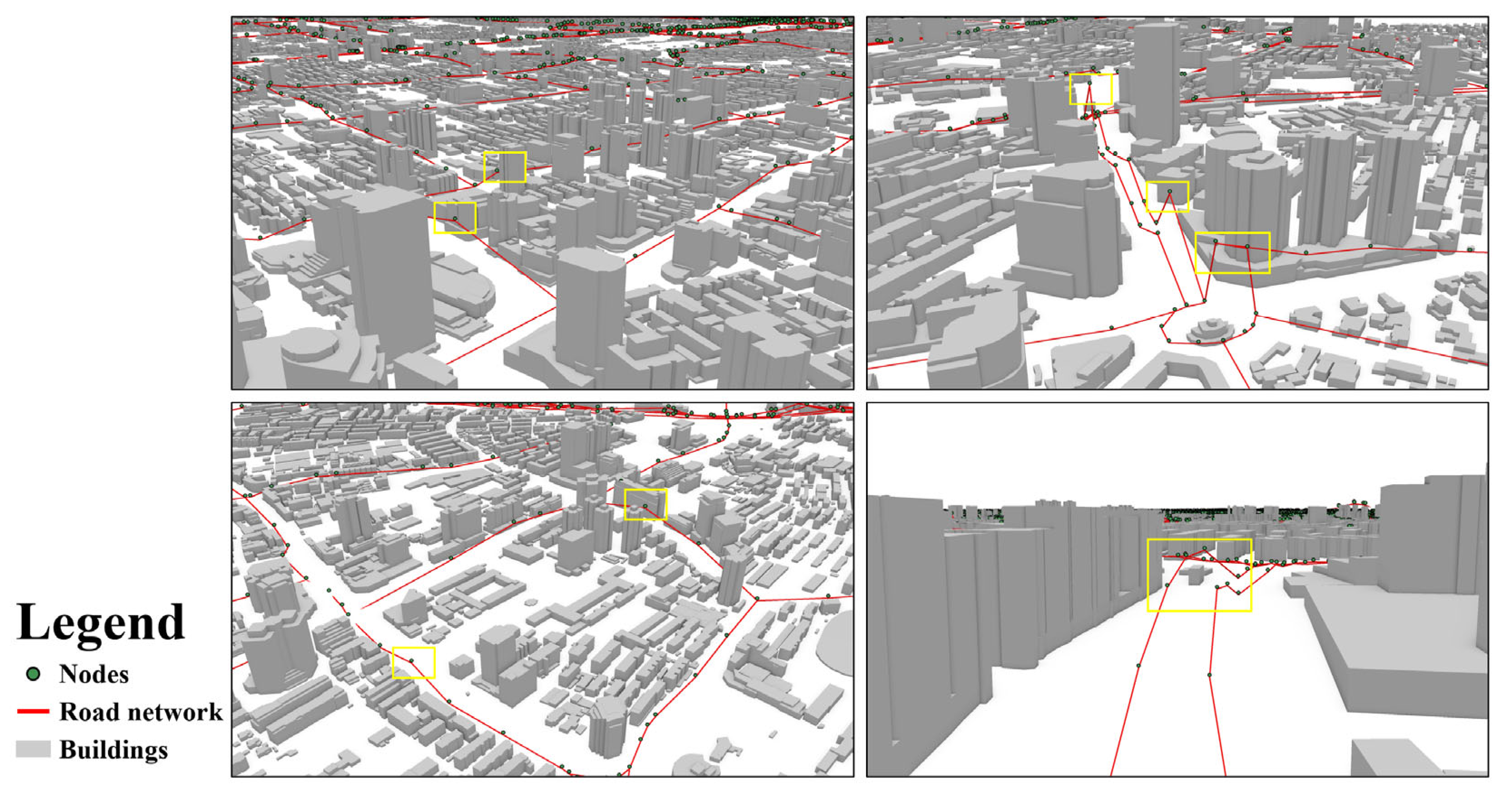
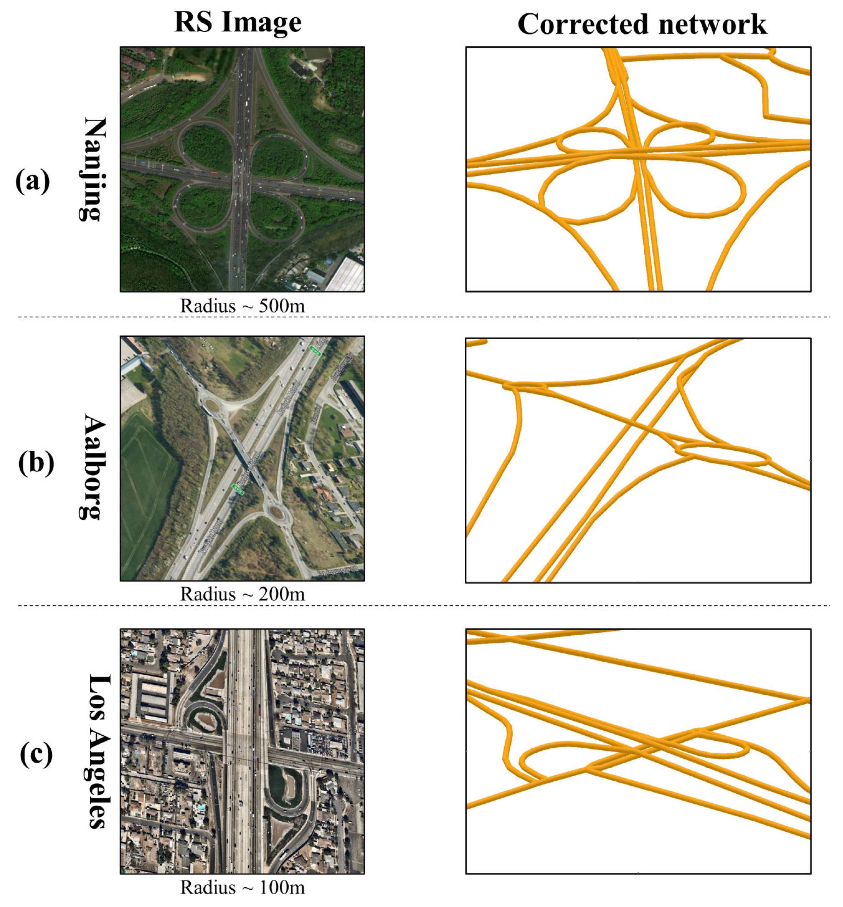
4.2. Topology Assessment of Road Network
5. Discussion
5.1. Spatial Distribution of Road Edge Elevation and Absolute Grades
5.2. Potential Developing Directions
6. Conclusions
Author Contributions
Funding
Data Availability Statement
Acknowledgments
Conflicts of Interest
References
- Barthelemy, M. From Paths to Blocks: New Measures for Street Patterns. Environ. Plan. B Urban Anal. City Sci. 2017, 44, 256–271. [Google Scholar] [CrossRef]
- Zhong, S.; Yang, X.; Chen, R. The accessibility measurement of hierarchy public service facilities based on multi-mode network dataset and the two-step 2SFCA: A case study of Beijing’s medical facilities. Geogr. Res. 2016, 35, 731–744. [Google Scholar]
- Kan, Z.; Tang, L.; Kwan, M.-P.; Ren, C.; Liu, D.; Li, Q. Traffic Congestion Analysis at the Turn Level Using Taxis’ GPS Trajectory Data. Comput. Environ. Urban Syst. 2019, 74, 229–243. [Google Scholar] [CrossRef]
- Herrera, J.C.; Work, D.B.; Herring, R.; Ban, X.; Jacobson, Q.; Bayen, A.M. Evaluation of Traffic Data Obtained via GPS-Enabled Mobile Phones: The Mobile Century Field Experiment. Transp. Res. Part C Emerg. Technol. 2010, 18, 568–583. [Google Scholar] [CrossRef] [Green Version]
- Wang, H.; Zeng, W.; Cao, R. Simulation of the Urban Jobs–Housing Location Selection and Spatial Relationship Using a Multi-Agent Approach. ISPRS Int. J. Geo-Inf. 2021, 10, 16. [Google Scholar] [CrossRef]
- Guo, Y.; Tang, Z.; Guo, J. Could a Smart City Ameliorate Urban Traffic Congestion? A Quasi-Natural Experiment Based on a Smart City Pilot Program in China. Sustainability 2020, 12, 2291. [Google Scholar] [CrossRef] [Green Version]
- Zhou, Q.; Zhang, W. A Preliminary Review on 3-Dimensional City Model. In Proceedings of the Asia GIS 2003 Conference, Wuhan, China, 16–18 October 2003; pp. 16–18. [Google Scholar]
- Ren, C.; Cai, M.; Li, X.; Shi, Y.; See, L. Developing a Rapid Method for 3-Dimensional Urban Morphology Extraction Using Open-Source Data. Sustain. Cities Soc. 2020, 53, 101962. [Google Scholar] [CrossRef]
- Fang, Z.; Qi, J.; Fan, L.; Huang, J.; Jin, Y.; Yang, T. A Topography-Aware Approach to the Automatic Generation of Urban Road Networks. Int. J. Geogr. Inf. Sci. 2022, 36, 2035–2059. [Google Scholar] [CrossRef]
- Badhrudeen, M.; Derrible, S.; Verma, T.; Kermanshah, A.; Furno, A. A Geometric Classification of World Urban Road Networks. Urban Sci. 2022, 6, 11. [Google Scholar] [CrossRef]
- Fan, C.; Jiang, X.; Mostafavi, A. A Network Percolation-Based Contagion Model of Flood Propagation and Recession in Urban Road Networks. Sci. Rep. 2020, 10, 13481. [Google Scholar] [CrossRef]
- Qing, Z.H.U.; Liguo, Z.; Yulin, D.; Han, H.U.; Xuming, G.E.; Mingwei, L.I.U.; Wei, W. From Real 3D Modeling to Digital Twin Modeling. Acta Geod. Cartogr. Sin. 2022, 51, 1040. [Google Scholar]
- Zhu, Q.; Li, Y. Hierarchical Lane-oriented 3D Road-network Model. Int. J. Geogr. Inf. Sci. 2008, 22, 479–505. [Google Scholar] [CrossRef]
- Yeh, A.G.-O.; Zhong, T.; Yue, Y. Angle Difference Method for Vehicle Navigation in Multilevel Road Networks with a Three-Dimensional Transport GIS Database. IEEE Trans. Intell. Transp. Syst. 2017, 18, 140–152. [Google Scholar] [CrossRef]
- Yang, L.; Yang, X.; Zhang, H.; Ma, J.; Zhu, H.; Huang, X. Urban Morphological Regionalization Based on 3D Building Blocks—A Case in the Central Area of Chengdu, China. Comput. Environ. Urban Syst. 2022, 94, 101800. [Google Scholar] [CrossRef]
- Tavares, G.; Zsigraiová, Z.; Semião, V.; Carvalho, M. Optimisation of MSW Collection Routes for Minimum Fuel Consumption Using 3D GIS Modelling. Waste Manag. 2008, 29, 1176–1185. [Google Scholar] [CrossRef] [PubMed]
- Guo, C.; Ma, Y.; Yang, B.; Jensen, C.S.; Kaul, M. Ecomark: Evaluating Models of Vehicular Environmental Impact. In Proceedings of the 20th International Conference on Advances in Geographic Information Systems, Redondo Beach, CA, USA, 7–9 November 2012; pp. 269–278. [Google Scholar]
- Katzorke, N. Using RTK-Based Automated Vehicles to Pre-Mark Temporary Road Marking Patterns for Test Maneuvers of Automated Vehicles. In Proceedings of the 2022 International Conference on Connected Vehicle and Expo (ICCVE), Lakeland, FL, USA, 7–9 March 2022; pp. 1–5. [Google Scholar]
- Yang, B.; Fang, L.; Li, J. Semi-Automated Extraction and Delineation of 3D Roads of Street Scene from Mobile Laser Scanning Point Clouds. ISPRS J. Photogramm. Remote Sens. 2013, 79, 80–93. [Google Scholar] [CrossRef]
- Kaul, M.; Yang, B.; Jensen, C. Building Accurate 3D Spatial Networks to Enable Next Generation Intelligent Transportation Systems. In Proceedings of the 2013 IEEE 14th International Conference on Mobile Data Management, Milan, Italy, 3–6 June 2013; Volume 1. [Google Scholar]
- Qian, C.; Gale, B.; Bach, J. Earth Documentation: Overpass Detection Using Mobile Lidar. In Proceedings of the 2010 IEEE International Conference on Image Processing, Hong Kong, China, 26–29 September 2010; IEEE: Piscataway, NJ, USA; pp. 3901–3904. [Google Scholar]
- Gao, L.; Shi, W.; Zhu, J.; Shao, P.; Sun, S.; Li, Y.; Wang, F.; Gao, F. Novel Framework for 3D Road Extraction Based on Airborne LiDAR and High-Resolution Remote Sensing Imagery. Remote Sens. 2021, 13, 4766. [Google Scholar] [CrossRef]
- Zhou, Y.; Huang, R.; Jiang, T.; Dong, Z.; Yang, B. Highway Alignments Extraction and 3D Modeling from Airborne Laser Scanning Point Clouds. Int. J. Appl. Earth Obs. Geoinformat. 2021, 102, 102429. [Google Scholar] [CrossRef]
- McKenzie, G.; Janowicz, K. ISED: Constructing a High-Resolution Elevation Road Dataset from Massive, Low-Quality in-Situ Observations Derived from Geosocial Fitness Tracking Data. PLoS ONE 2017, 12, e0186474. [Google Scholar] [CrossRef] [Green Version]
- Yang, Z.; Zhang, Q. Low-Cost and Accurate 3D Road Modeling Using Mobile Phone. IEEE Trans. Mob. Comput. 2016, 15, 2494–2506. [Google Scholar] [CrossRef]
- Shu, J.; Wang, S.; Jia, X.; Zhang, W.; Xie, R.; Huang, H. Efficient Lane-Level Map Building via Vehicle-Based Crowdsourcing. IEEE Trans. Intell. Transp. Syst. 2022, 23, 4049–4062. [Google Scholar] [CrossRef]
- Wang, J. Automatic High-Fidelity 3D Road Network Modeling. Ph.D. Thesis, Old Dominion University, Norfolk, VA, USA, 2011. [Google Scholar] [CrossRef]
- Schpok, J. Geometric Overpass Extraction from Vector Road Data and DSMs. In Proceedings of the 19th ACM SIGSPATIAL International Conference on Advances in Geographic Information Systems; Association for Computing Machinery: New York, NY, USA, 2011; pp. 3–8. [Google Scholar]
- Wang, Y.; Zou, Y.; Henrickson, K.; Wang, Y.; Tang, J.; Park, B.-J. Google Earth Elevation Data Extraction and Accuracy Assessment for Transportation Applications. PLoS ONE 2017, 12, e0175756. [Google Scholar] [CrossRef] [PubMed] [Green Version]
- Li, L. 3D Road Network Extraction Method Based on UAV Oblique Photography. China J. Highw. Transp. 2019, 32, 219–226, 254. [Google Scholar]
- Tachikawa, T.; Hato, M.; Kaku, M.; Iwasaki, A. Characteristics of ASTER GDEM Version 2. In Proceedings of the 2011 IEEE International Geoscience and Remote Sensing Symposium, Vancouver, BC, Canada, 24–29 July 2011; pp. 3657–3660. [Google Scholar]
- Farr, T.G.; Rosen, P.A.; Caro, E.; Crippen, R.; Duren, R.; Hensley, S.; Kobrick, M.; Paller, M.; Rodriguez, E.; Roth, L. The Shuttle Radar Topography Mission. Rev. Geophys. 2007, 45, RG2004. [Google Scholar] [CrossRef] [Green Version]
- Zhang, X.; Zhong, M.; Liu, S.; Zheng, L.; Chen, Y. Template-Based 3D Road Modeling for Generating Large-Scale Virtual Road Network Environment. ISPRS Int. J. Geo-Inf. 2019, 8, 364. [Google Scholar] [CrossRef] [Green Version]
- Over, M.; Schilling, A.; Neubauer, S.; Zipf, A. Generating Web-Based 3D City Models from OpenStreetMap: The Current Situation in Germany. Comput. Environ. Urban Syst. 2010, 34, 496–507. [Google Scholar] [CrossRef]
- Wang, H.; Wu, Y.; Han, X.; Xu, M.; Chen, W. Automatic Generation of Large-Scale 3D Road Networks Based on GIS Data. Comput. Graph. 2021, 96, 71–81. [Google Scholar] [CrossRef]
- Tang, G.-A. Progress of DEM and Digital Terrain Analysis in China. Acta Geogr. Sin. 2014, 69, 1305–1325. [Google Scholar]
- Xiong, L.; Li, S.; Tang, G.; Strobl, J. Geomorphometry and Terrain Analysis: Data, Methods, Platforms and Applications. Earth-Sci. Rev. 2022, 233, 104191. [Google Scholar] [CrossRef]
- Santillan, J.R.; Makinano-Santillan, M. Vertical Accuracy Assessment of 30-M Resolution Alos, Aster, and Srtm Global Dems Over Northeastern Mindanao, Philippines. Int. Arch. Photogramm. Remote Sens. Spat. Inf. Sci. 2016, XLI-B4, 149–156. [Google Scholar] [CrossRef] [Green Version]
- Guth, P.L.; Geoffroy, T.M. LiDAR Point Cloud and ICESat-2 Evaluation of 1 Second Global Digital Elevation Models: Copernicus Wins. Trans. GIS 2021, 25, 2245–2261. [Google Scholar] [CrossRef]
- Nikolakopoulos, K.G. Accuracy Assessment of ALOS AW3D30 DSM and Comparison to ALOS PRISM DSM Created with Classical Photogrammetric Techniques. Eur. J. Remote Sens. 2020, 53, 39–52. [Google Scholar] [CrossRef]
- Stilla, U.; Soergel, U.; Thoennessen, U. Potential and Limits of InSAR Data for Building Reconstruction in Built-up Areas. ISPRS J. Photogramm. Remote Sens. 2003, 58, 113–123. [Google Scholar] [CrossRef]
- Vargas-Munoz, J.E.; Srivastava, S.; Tuia, D.; Falcão, A.X. OpenStreetMap: Challenges and Opportunities in Machine Learning and Remote Sensing. IEEE Geosci. Remote Sens. Mag. 2021, 9, 184–199. [Google Scholar] [CrossRef]
- Irshad, M.E.; Sohail, H.; Zafar, N.; Haq, I.U. A Framework for Synthesizing Tracker Speeds on Open Street Maps. In Proceedings of the 2020 IEEE 23rd International Multitopic Conference (INMIC), Bahawalpur, Pakistan, 5–7 November 2020; pp. 1–6. [Google Scholar]
- Chakeri, A.; Wang, X.; Goss, Q.; Akbas, M.I.; Jaimes, L.G. A Platform-Based Incentive Mechanism for Autonomous Vehicle Crowdsensing. IEEE Open J. Intell. Transp. Syst. 2021, 2, 13–23. [Google Scholar] [CrossRef]
- Boeing, G. OSMnx: New Methods for Acquiring, Constructing, Analyzing, and Visualizing Complex Street Networks. Comput. Environ. Urban Syst. 2017, 65, 126–139. [Google Scholar] [CrossRef] [Green Version]
- Takaku, J.; Tadono, T.; Tsutsui, K. Generation of High Resolution Global DSM from ALOS PRISM. Int. Arch. Photogramm. Remote Sens. Spat. Inf. Sci. 2014, XL-4, 243–248. [Google Scholar] [CrossRef] [Green Version]
- Tadono, T.; Ishida, H.; Oda, F.; Naito, S.; Minakawa, K.; Iwamoto, H. Precise Global DEM Generation by ALOS PRISM. ISPRS Ann. Photogramm. Remote Sens. Spat. Inf. Sci. 2014, II-4, 71–76. [Google Scholar] [CrossRef] [Green Version]
- Huang, H.; Chen, P.; Xu, X.; Liu, C.; Wang, J.; Liu, C.; Clinton, N.; Gong, P. Estimating Building Height in China from ALOS AW3D30. ISPRS J. Photogramm. Remote Sens. 2022, 185, 146–157. [Google Scholar] [CrossRef]
- Nonomura, A.; Hasegawa, S.; Kanbara, D.; Tadono, T.; Chiba, T. Topographic Analysis of Landslide Distribution Using AW3D30 Data. Geosciences 2020, 10, 115. [Google Scholar] [CrossRef] [Green Version]
- Xu, Y.; Zhang, S.; Li, J.; Liu, H.; Zhu, H. Extracting Terrain Texture Features for Landform Classification Using Wavelet Decomposition. ISPRS Int. J. Geo-Inf. 2021, 10, 658. [Google Scholar] [CrossRef]
- Hawker, L.; Uhe, P.; Paulo, L.; Sosa, J.; Savage, J.; Sampson, C.; Neal, J. A 30 m Global Map of Elevation with Forests and Buildings Removed. Environ. Res. Lett. 2022, 17, 024016. [Google Scholar] [CrossRef]
- Marešová, J.; Gdulová, K.; Pracná, P.; Moravec, D.; Gábor, L.; Prošek, J.; Barták, V.; Moudrý, V. Applicability of Data Acquisition Characteristics to the Identification of Local Artefacts in Global Digital Elevation Models: Comparison of the Copernicus and TanDEM-X DEMs. Remote Sens. 2021, 13, 3931. [Google Scholar] [CrossRef]
- OpenStreetMap contributors Planet Dump. 2017. Available online: https://planet.osm.org (accessed on 1 September 2022).
- Hagberg, A.; Swart, P.; Chult, S.D. Exploring Network Structure, Dynamics, and Function Using Networkx. In Proceedings of the SCIPY 08; Pasadena, CA, USA, 21 August 2008, Los Alamos National Lab (LANL): Los Alamos, NM, USA, 2008. [Google Scholar]
- American Association of State Highway and Transportation Official (AASHTO). A Policy on Geometric Design of Highways and Streets 2018, 7th ed.; American Association of State Highway and Transportation Officials: Washington, DC, USA, 2021. [Google Scholar]
- Technical Standard for Highway Engineering in Suburban and Rural Town Areas; Ministry of Transport of the People’s Republic of China: Beijing, China, 2021.
- California, S. of Highway Design Manual (HDM) | Caltrans. Available online: https://dot.ca.gov/programs/design/manual-highway-design-manual-hdm (accessed on 15 September 2022).
- Wang, X.; You, S.; Wang, L. Classifying Road Network Patterns Using Multinomial Logit Model. J. Transp. Geogr. 2017, 58, 104–112. [Google Scholar] [CrossRef] [Green Version]
- Girres, J.-F.; Touya, G. Quality Assessment of the French OpenStreetMap Dataset. Trans. GIS 2010, 14, 435–459. [Google Scholar] [CrossRef]
- Liu, H.; Xu, Y.; Tang, J.; Deng, M.; Huang, J.; Yang, W.; Wu, F. Recognizing Urban Functional Zones by a Hierarchical Fusion Method Considering Landscape Features and Human Activities. Trans. GIS 2020, 24, 1359–1381. [Google Scholar] [CrossRef]
- Burghardt, K.; Uhl, J.H.; Lerman, K.; Leyk, S. Road Network Evolution in the Urban and Rural United States since 1900. Comput. Environ. Urban Syst. 2022, 95, 101803. [Google Scholar] [CrossRef]
- Xue, J.; Jiang, N.; Liang, S.; Pang, Q.; Yabe, T.; Ukkusuri, S.V.; Ma, J. Quantifying the Spatial Homogeneity of Urban Road Networks via Graph Neural Networks. Nat. Mach. Intell. 2022, 4, 246–257. [Google Scholar] [CrossRef]
- Zhong, T.; Zhang, K.; Chen, M.; Wang, Y.; Zhu, R.; Zhang, Z.; Zhou, Z.; Qian, Z.; Lv, G.; Yan, J. Assessment of Solar Photovoltaic Potentials on Urban Noise Barriers Using Street-View Imagery. Renew. Energy 2021, 168, 181–194. [Google Scholar] [CrossRef]
- Zahedi, R.; Ghorbani, M.; Daneshgar, S.; Gitifar, S.; Qezelbigloo, S. Potential Measurement of Iran’s Western Regional Wind Energy Using GIS. J. Clean. Prod. 2022, 330, 129883. [Google Scholar] [CrossRef]
- Singh, P.; Sinha, V.S.P.; Vijhani, A.; Pahuja, N. Vulnerability Assessment of Urban Road Network from Urban Flood. Int. J. Disaster Risk Reduct. 2018, 28, 237–250. [Google Scholar] [CrossRef]
- Rey Gozalo, G.; Suárez, E.; Montenegro, A.L.; Arenas, J.P.; Barrigón Morillas, J.M.; Montes González, D. Noise Estimation Using Road and Urban Features. Sustainability 2020, 12, 9217. [Google Scholar] [CrossRef]
- Zeng, L.; Lu, J.; Li, W.; Li, Y. A Fast Approach for Large-Scale Sky View Factor Estimation Using Street View Images. Build. Environ. 2018, 135, 74–84. [Google Scholar] [CrossRef]
- Huang, X.; Wang, Y. Investigating the Effects of 3D Urban Morphology on the Surface Urban Heat Island Effect in Urban Functional Zones by Using High-Resolution Remote Sensing Data: A Case Study of Wuhan, Central China. ISPRS J. Photogramm. Remote Sens. 2019, 152, 119–131. [Google Scholar] [CrossRef]
- Jordahl, K.; den Bossche, J.V.; Fleischmann, M.; McBride, J.; Wasserman, J.; Richards, M.; Badaracco, A.G.; Gerard, J.; Snow, A.D.; Tratner, J.; et al. Geopandas/Geopandas: V0.11.0 2022. Zenodo. [CrossRef]


| Type of Terrain | Freeways and Expressways | Rural Highways | Urban Highways |
|---|---|---|---|
| Level | 3% | 4% | 6% |
| Rolling | 4% | 5% | 7% |
| Mountainous | 6% | 7% | 9% |
| Designed Speed (km/h) | Maximum Grades (%) |
|---|---|
| 120 | 3 |
| 100 | 3 |
| 80 | 4 |
| 60 | 5 |
| 50 | 5.5 |
| 40 | 6 |
| 30 | 7 |
| 20 | 8 |
Publisher’s Note: MDPI stays neutral with regard to jurisdictional claims in published maps and institutional affiliations. |
© 2022 by the authors. Licensee MDPI, Basel, Switzerland. This article is an open access article distributed under the terms and conditions of the Creative Commons Attribution (CC BY) license (https://creativecommons.org/licenses/by/4.0/).
Share and Cite
Chen, Y.; Yang, X.; Yang, L.; Feng, J. An Automatic Approach to Extracting Large-Scale Three-Dimensional Road Networks Using Open-Source Data. Remote Sens. 2022, 14, 5746. https://doi.org/10.3390/rs14225746
Chen Y, Yang X, Yang L, Feng J. An Automatic Approach to Extracting Large-Scale Three-Dimensional Road Networks Using Open-Source Data. Remote Sensing. 2022; 14(22):5746. https://doi.org/10.3390/rs14225746
Chicago/Turabian StyleChen, Yang, Xin Yang, Ling Yang, and Jiayu Feng. 2022. "An Automatic Approach to Extracting Large-Scale Three-Dimensional Road Networks Using Open-Source Data" Remote Sensing 14, no. 22: 5746. https://doi.org/10.3390/rs14225746