Clues of Ongoing Deep Magma Inflation at Campi Flegrei Caldera (Italy) from Empirical Orthogonal Function Analysis of SAR Data

Abstract

Understanding the characteristics of a volcanic system is always important and becomes crucial when the volcano is in pluri-decadal unrest and located in a densely populated area, such as Campi Flegrei caldera, Italy. Ground deformation is a powerful source of information for studying the activity of magmatic sources and hydrothermal systems, even when difficult to detect otherwise. Here, we use ground displacement from ERS-ENVISAT and Sentinel-1A SAR images to investigate the 1993–2000 subsidence and part (2015–2022) of the present unrest. For each of the two time periods, we combine the line-of-sight displacements to obtain vertical and eastward displacements, and apply the empirical orthogonal function analysis to these latter time series—treated as a single data set—to decompose space-time fields into separated modes, consisting of uncorrelated spatial patterns and associated temporal evolutions. We only retain the first mode, since it captures the main deformation during both investigated periods, is the sole mode related to long-lasting (years) processes, and is less affected by noise than original data. Our analyses: (i) Confirm that most of the deformation is related to the activity of a 3–4 km deep sill-like source, which is inflated by magma and/or magmatic fluids during periods of unrest and deflates during periods of subsidence; (ii) Evidence ongoing deformation linked to local fluid migration in the Solfatara area; (iii) Identify persistent deformation features where peculiar fluid migration processes occurred during the 1982–1984 unrest; (iv) Most importantly, provide direct evidence of deep magma inflation at least since 2015, thus giving a strong warning of increasing risk at Campi Flegrei. Results demonstrate the capability of our approach to disclose hardly detectable processes and suggest a tool to monitor the activity of the deep magmatic source. Our approach can be useful also in other volcanic systems.

1. Introduction

Campi Flegrei is a nested caldera related to two main eruptive events, the Campanian Ignimbrite eruption (about 39 ka) and the Neapolitan Yellow tuff eruption (about 15 ka) (e.g., [1,2]). It is located within a densely populated volcanic region to the west of Naples (about 3 million inhabitants) and is one of the most hazardous area in the world. The last 15 ka were accompanied by several tens of eruptions (at least 60) and resurgence of the caldera center; the caldera-wide uplift has been largest in the coastal town of Pozzuoli (Pozzuoli area, P in Figure 1). The last eruption (Monte Nuovo, MN in Figure 1) occurred in 1538 AD, after about 3 ka of quiescence, more than 1 ka of subsidence from the Roman times, and a period of increasing seismicity and uplift from about 1400 to 1536; the eruption was followed by deflation.

Campi Flegrei caldera is renowned for its continual slow vertical movements (bradyseism) and is in intermittent unrest since the 1950s. At least three major unrest episodes occurred between 1950–1952, 1969–1972, and 1982–1984, followed by long-lasting subsidence overlapped by a few short uplift phases. Since 2005, the Campi Flegrei area is mostly rising at an accelerating rate [4] and the uplift has raised again Pozzuoli to about its 1984 level (e.g., Figure 2). The Solfatara fumarolic area (SF in Figure 1) is currently experiencing an escalation in fluid release at the surface (e.g., [7]), as a result of massive magma degassing in the deep portion of the plumbing system (e.g., [8]). There is no general consensus about the nature—magmatic, hydrothermal or hybrid—of Campi Flegrei unrests; in all cases, they appear to belong to an evolving sequence of long-term disturbance in the magmatic system (e.g., [9]).

Understanding the processes that take place at Campi Flegrei is of major importance not only for the scientific knowledge of an intriguing volcanic area, but also for assessing future unrest hazard. A comprehensive view of its dynamics should take into account deformation, seismicity, gravity data, changes of geochemical indicators, crustal structures and the (at least simplified) source of each observable; obviously, inferences from different data should be consistent with each other, and possible spatial and temporal correlation between different geophysical and geochemical/petrological data would help to clarify sources of deformation, seismicity and geochemical changes.

Without demanding completeness, we mention that the physical processes that take place at Campi Flegrei are probably the result of interactions between the superficial hydrothermal system, magmatic-related source(s) at intermediate depths and deep magmatic source(s)—between the deep source and the magmatic-related intermediate one (e.g., [10,11]), between the magmatic-related intermediate source and the hydrothermal system (e.g., [6,12]), between an ∼8-km-deep source and the hydrothermal system (e.g., [13,14]), between an even deeper source, the ∼8-km-deep one, and the hydrothermal system (e.g., [8,14]). All aspects have been abundantly studied and the literature on Campi Flegrei is immense, mainly as regards the dynamics after 1980; thus, only what is needed to contextualize the deformation data analyses in this work and our results is outlined here.

As for the major 1982–1984 unrest, deformation data from leveling and geodetic precise-traversing surveys (electronic distance and angular measurements) are satisfied by inflation of a horizontal sill (PTE in Figure 1), centered offshore Pozzuoli at about 3–4 km depth [5,10]. Although it is obviously a simplification, 1980–2013 geodetic data—including continuous Global Positioning System (GPS) data and Synthetic Aperture Radar (SAR) images—indicate that the deformation history during the whole period is mostly satisfied by two simple paired deformation sources for both inflation and deflation phases [5,15]. Large-scale deformation can be explained almost completely by inflation/deflation of the PTE, whose location is consistent with the 3–4 km deep coda-wave high-attenuation patch detected under Pozzuoli [16]. The PTE can be fed by magma and/or magmatic fluids from the partially molten zone detected beneath the caldera at depth larger than 7.5 km (e.g., [17,18]). Almost all the residual deformation is confined to the area of the Solfatara fumarolic field—not covered by leveling surveys before 1983—and can be explained by a local source (PS in Figure 1). The PS can be thought in terms of hydrothermally driven poroelastic deformation [19] near the injection point of hot magmatic fluids into the hydrothermal system.

As for the major 1983–1984 unrest, seismic analyses have enlightened [6]: (i) The seismicity related to the paired deformation sources in [5]; (ii) The seismic evidence of repeated daily fluid injections modeled by [12] (RFI in Figure 1); (iii) The connection of the 3–4 km deep high-attenuation reservoir under Pozzuoli with the fumaroles at Mofete and Monte Nuovo (M and MN in Figure 1, PMC indicates where the spatial 1983–1984 seismic pattern turns from E-W to NW-SE); (iv) The release of fluids which reached Solfatara from the the 3–4 km deep reservoir; (v) The stress release that halted the seismic unrest. Until now, there is no evidence of deformation anomalies in the areas where the repeated fluid injections and the opening of the Pozzuoli-Monte Nuovo pathway were envisaged; furthermore—and much more important—there is no deformation evidence of the deep source activity.

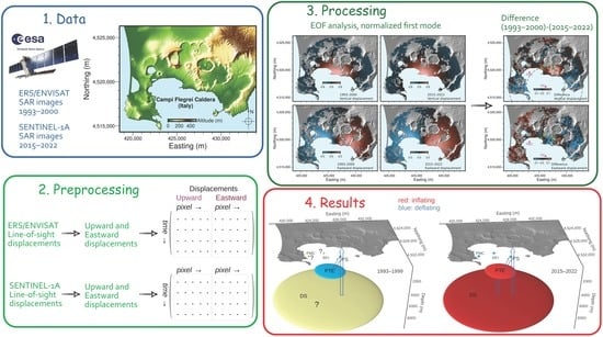
In this work, we show that long-lasting (years) faint deformation signatures of various complex processes—related to the dynamics of the different portions of the plumbing system, from the hydrothermal system to the deeper source—can be revealed by proper analyses of deformation data. Of most importance is the detection of the arrival of fresh, mafic hot magma from the mantle, inflating the deeper source. We use ground displacement time series obtained from ERS-ENVISAT ([20]) and Sentinel-1A ([21]) SAR images, spanning 1993–2000 and 2015–2022, respectively. We apply the empirical orthogonal function analysis to SAR data inside the circular region bounded by the black dashed circle in Figure 1. Our analyses: confirm that most of the deformation is related to the activity of a sill-like source at 3–4 km depth; confirm the deformation anomaly (excess of subsidence) at Solfatara during 1993–2000; indicate that the Solfatara area is uplifting at a lower rate than the surroundings since 2015; identify persistent deformation features close to RFI and PMC; and, most importantly, give evidence of deep inflation at least since 2015.

2. Materials and Methods

2.1. SAR Data and Analysis

We use ground displacement time series obtained from ERS-ENVISAT ([20]) and Sentinel-1A ([21]) SAR images. We refer displacements to the median value inside a circular area, 500 m in radius, centered on LR (Figure 1).

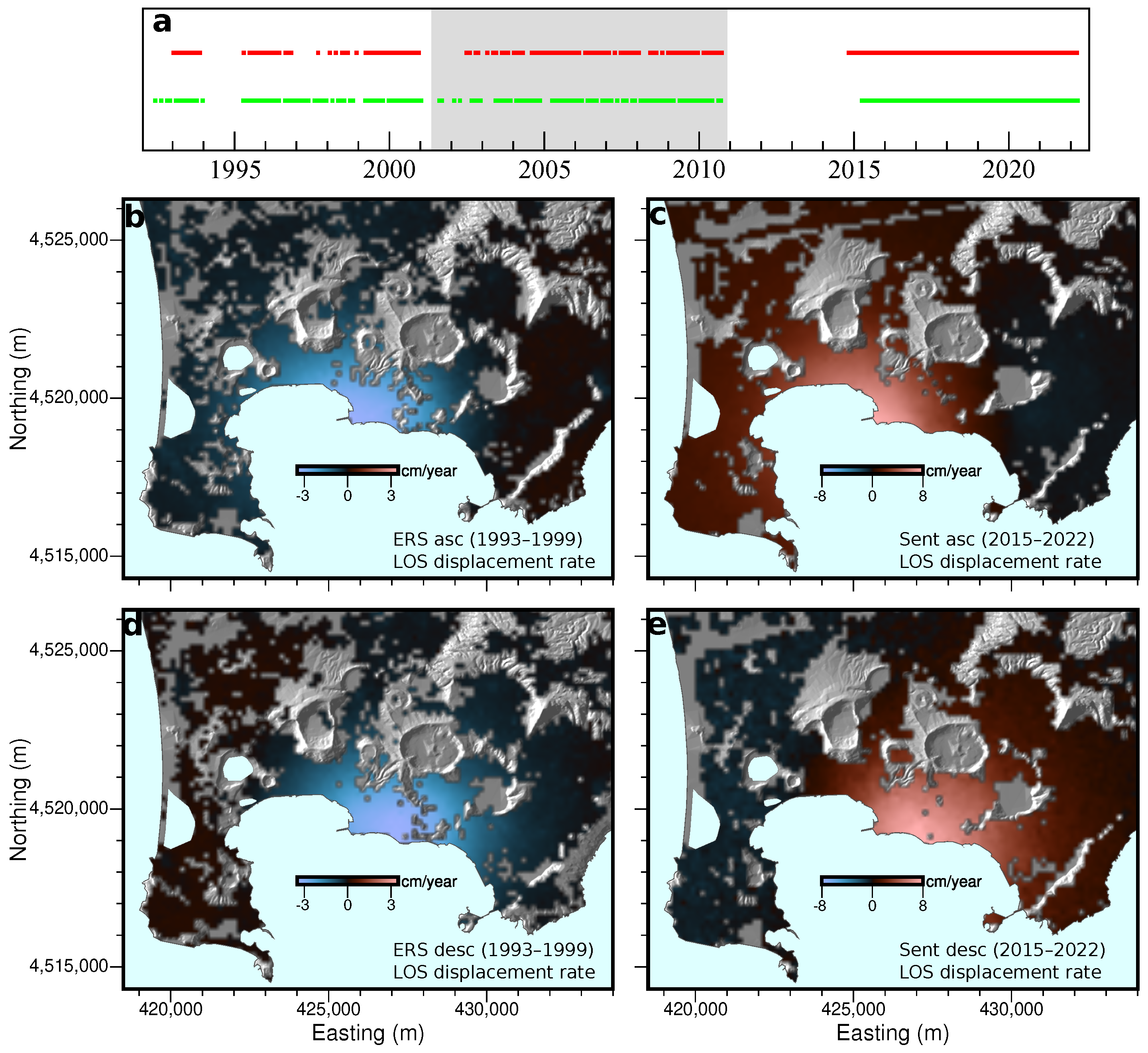
As for ERS-ENVISAT data, we use a subset of the line-of-sight (LOS) displacement time series in [5], obtained through the Small BAseline Subset Differential Synthetic Aperture Radar Interferometry (SBAS DInSAR) technique ([22]). The time series include 138 ascending-orbit images from 1993.03 to 2010.73 and 155 descending-orbit images from 1992.44 to 2010.71 (Figure 3a). The angle between the LOS direction and the vertical (i.e., the incidence angle) in the study area is about 23${}^{°}$ for the ascending orbit and 21${}^{°}$ for the descending orbit. The temporal interferometric coherence of the time series is larger than 0.55 for the ascending orbit and 0.5 for the descending orbit. To decrease the amount of data and noise, we spatially filter and decimate each map of the LOS time series by computing a median value for every non-empty block in a regular (150 m × 150 m) grid. Figure 3b,d show the mean LOS displacement rate during 1993–1999, i.e., before the onset of the 2000 mini-uplift (see Figure 2a).

As for Sentinel-1A data, we use Level-1 Single Look Complex (SLC) Sentinel-1A interferometric wide swath imagery [23], provided by the European Space Agency (ESA) and downloaded from the Alaska Satellite Facility [24]. SLC products consist of focused SAR data, that are geo-referenced using orbit and attitude data from the satellite and provided in slant-range geometry. The time series include 193 ascending-orbit images from 2014.84 to 2022.22 and 192 descending-orbit images from 2015.26 to 2022.19 (Figure 3a). The incidence angle in the study area is about 35.6${}^{°}$ for the ascending orbit and 35${}^{°}$ for the descending orbit. We created times series of ascending-orbit and descending-orbit images using SBAS within GMTSAR InSAR processing system, version 11 July 2022 ([25]), through the Sentinel TOPS-mode processing and interferometry procedure. Main steps to make LOS time series are: image alignment and registration, enhanced spectral diversity, elevation antenna pattern correction, interferogram processing, and SBAS, after selecting image couples having temporal baseline shorter than 90 days and spatial baseline smaller than 50 m. We also mask out low coherence areas (e.g., wet and densely vegetated areas) and discard image couples whose mean interferometric correlation is smaller than 0.35 out of the masked areas. At last, we spatially filter and decimate each map of the LOS time series by computing a median value for every non-empty block in a regular (150 m × 150 m) grid. The resulting gridded time series are validated against continuous GPS data [4] acquired at several stations located in the Neapolitan Volcanic Area. As digital elevation model (DEM) we use TINITALY/01 (10 m-cell size grid [3]). Figure 3c,e show the mean LOS displacement rate during 2015–2022. We have also carried out some tests including correction for radar phase delays due to atmospheric propagation [26]; however, differences with uncorrected time series are so small that we do not further consider the displacement time series obtained including the atmospheric correction.

LOS displacements from ascending and descending orbits are combined as follows to obtain vertical and eastward displacements. First, we select ascending- and descending-orbit SAR acquisitions whose lag is shorter than 1 week (ERS-ENVISAT) or 1 day (Sentinel-1A) and generate a set of LOS–displacement map couples (times given in Figure 4a). Then, we combine gridded ascending and descending LOS displacements for each map couple, neglecting the small northward LOS components. Figure 4b–e show the mean upward and eastward displacement rates. Figure 5 compares Sentinel-1A vertical and eastward displacements with GPS displacements for the stations located inside the circular region bounded by the black dashed circle in Figure 1.

2.2. EOF Analysis

We apply the empirical orthogonal function (EOF) analysis to the SAR displacement time series inside the circular region bounded by the black dashed circle in Figure 1. EOF analysis decomposes a space-time field into spatial patterns and associated temporal evolutions, and is commonly used to detect spatial and temporal changes in climatic modes ([27]). This technique is also known as principal component analysis (PCA) and was applied to Campi Flegrei for denoising SAR data in [28].

For a time series of $n_t$ displacement maps each of $n_p$ pixels, data can be arranged in a $n_t\times n_p$ matrix (spatial organization) or $n_p\times n_t$ matrix (temporal organization). In this work we organize data spatially—putting together vertical and eastward displacements in a single $n_t\times 2n_p$ data matrix—because we search for uncorrelated spatial patterns of vertical and eastward displacements which share the same temporal evolutions.

We separately subtract the mean value to the upward and eastward displacement in each corresponding row of the original $n_t\times 2n_p$ data matrix so as to have zero mean “relative” (with respect to the mean) upward and eastward displacement vectors at each time, and obtain a new $n_t\times 2n_p$ data matrix $\mathbf{X}$. Data could be also normalized by dividing each column of $\mathbf{X}$ by its standard deviation; doing so, pixels are considered equally important, and as a result, the spatial patterns will try to describe the overall variation of the deformation field. If data are not normalized, spatial patterns will try to optimize the variation of the deformation field in the regions of highest standard deviation; spatial patterns from non-normalized data are usually of simpler physical interpretation and we decide to avoid normalization.

We factorize $\mathbf{X}$ into three matrices by singular value decomposition using svd() function in Octave programming tool, thus $\mathbf{X}=\mathbf{U}\mathbf{D}{\mathbf{V}}^T$, where $\mathbf{U}$ and $\mathbf{V}$ are orthonormal, i.e., $\mathbf{U}{\mathbf{U}}^T={\mathbf{U}}^T\mathbf{U}=\mathbf{I}$ and $\mathbf{V}{\mathbf{V}}^T={\mathbf{V}}^T\mathbf{V}=\mathbf{I}$, $\mathbf{D}$ contains the singular values and is diagonal, i.e., all entries whose column number is different from the row number are zero, and $\mathbf{I}$ is the identity matrix; superscript T denotes transpose. Squared singular values are also the eigenvalues of the covariance matrix $\mathbf{S}=\mathbf{X}{\mathbf{X}}^T=\mathbf{U}{\mathbf{D}}^2{\mathbf{U}}^T$.

Since data are spatially organized, $\mathbf{U}$, $\mathbf{V}$ and $\mathbf{D}$ are $n_t\times n_t$, $2n_p\times 2n_p$ and $n_t\times 2n_p$ matrices, respectively. Columns of $\mathbf{V}$ give uncorrelated spatial patterns, and columns of $\mathbf{U}\mathbf{D}$ give related temporal evolutions; each column of $\mathbf{V}$ and $\mathbf{U}\mathbf{D}$ represents a mode. The displacement at pixel j and time $t_i$ related to mode m is given by ${\left(\mathbf{U}\mathbf{D}\right)}_{im}{\mathbf{V}}_{jm}$; thus, if ${\mathbf{V}}_{jm}>0$ then the displacement at pixel j follows the same temporal evolution as the mode, while if ${\mathbf{V}}_{jm}<0$ then the displacement at pixel j follows an opposite temporal evolution.

EOFs, i.e., the columns of $\mathbf{V}$, are given in descending order of the singular values, which means in descending order of importance. Generally speaking, the mathematical properties of the EOFs imply that each component may not have individual—dynamical, kinematic, statistical—meaning independent of other EOF modes; however, careful inspection of spatial patterns, temporal evolutions and singular values may allow to discern possible mode contamination. We separately apply the EOF analysis to the displacement ERS-ENVISAT time series from 1993 to end 2000 and to the Sentinel-1A ones from 2015 to 2022, focusing on the first mode.

2.3. Modeling

As outlined in Section 1, different processes may cause deformation at Campi Flegrei. Accurate realistic modeling of those processes and induced deformation is practically impossible because of the complexities of the processes and the medium; however, seismic tomography (e.g., [17]) shows that a layered model is a first-order effective approximation of the real rock heterogeneities beneath Campi Flegrei. Rock heterogeneity affects superficial deformation even for layered media; the presence of soft superficial layers above a source causes it to appear shallower (“focusing effect”, e.g., [10,29]) and amplifies horizontal-to-vertical displacement ratio [30]. Thus, we decided to use simple models of the deformation sources and the medium, and look for deformation evidences of previously suggested processes acting at Campi Flegrei.

Tested sources are embedded in an elastic homogeneous isotropic flat half-space; Poisson ratio is 0.25. As for the deformation sources, since most of the deformation is due to a quasi-circular horizontal sill—the PTE in [5]—and, to a minor extent, to a source which is approximately equivalent to a pressurized vertical oblate spheroid—the PS in [5]—we only consider pressurized circular horizontal sills and vertical (prolate or oblate) spheroids as effective—i.e., giving deformation patterns similar to the real ones—deformation sources. Deformation from circular horizontal sills is computed as in [31] by using the Matlab code available in dMODELS collection [32]. As for prolate or oblate spheroids, we use the approach in [33]. We schematize the PTE and the deep reservoir (DS) as circular horizontal sills, the PS as oblate spheroid and the RFI and PMC as vertical spheroids. To account—at least approximately—for the effects of rock layering on the horizontal-to-vertical displacement ratio, we multiply horizontal displacements by 1.5 or 1.3 if the deformation source is deeper or shallower than 3 km, respectively [30].

2.4. Differences between Subsidence and Uplift Spatial Patterns

To see if the deformation sources during subsidence (1993–2000) are the same as during uplift (2015–2022) and reveal possible differences, we compare the deformation spatial pattern obtained from ERS/ENVISAT data with that from Sentinel-1A data. Comparison is carried out as follows.

• We prepare two separate $n_t\times 2n_p$ data matrices, each consisting of upward and eastward relative displacements (i.e., pixel-wise mean is null at each time, Section 2.2) inside the circular region bounded by the dashed black circle in Figure 1, from ERS/ENVISAT and Sentinel-1A data, respectively.
• We apply the EOF analysis to each data matrix.
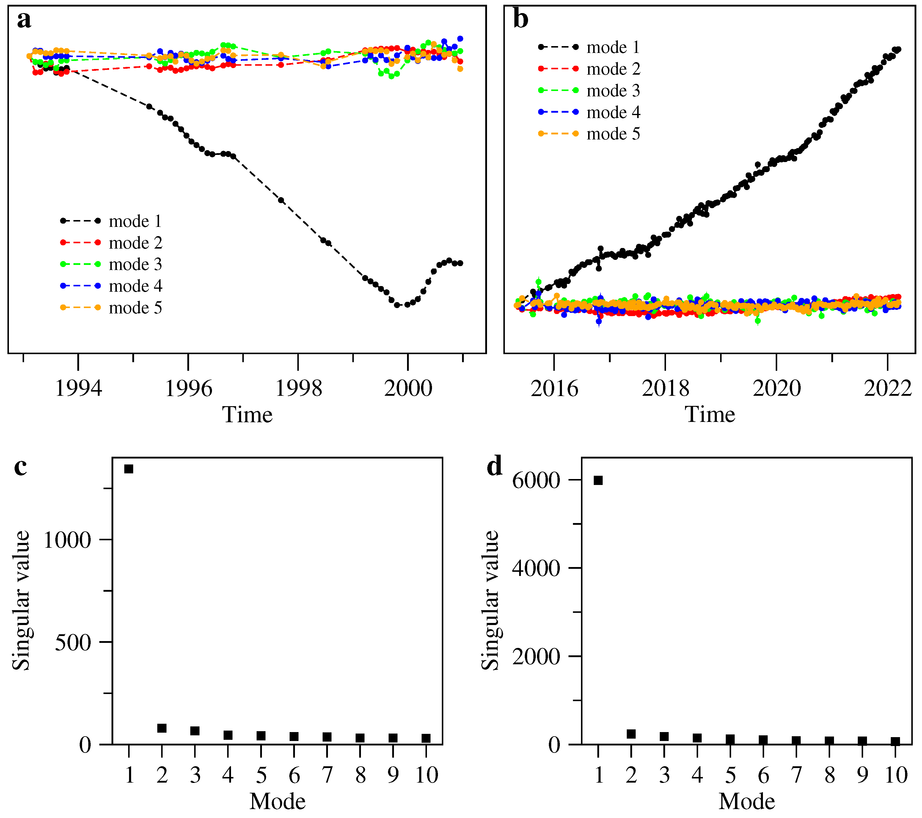
• We retain only EOFs related to the first mode, which captures the main deformation during both investigated periods (Figure 6c,d) and is the sole mode clearly related to long-lasting (years) processes (Figure 6a,b). Positive EOF elements indicate downward or westward relative displacement during 1993–2000 and upward or eastward relative displacement during 2015–2022, because related temporal evolutions represent subsidence and uplift, respectively (Figure 6a,b); the opposite holds for negative values.
• From the first mode EOFs we generate four datasets: (i) 1993–2000 vertical relative displacements ($h_{1,j}^v,j=1,\dots ,n_p$), (ii) 1993–2000 eastward relative displacements ($h_{1,j}^e,j=1,\dots ,n_p$), (iii) 2015–2022 vertical relative displacements ($h_{2,j}^v,j=1,\dots ,n_p$), (iv) 2015–2022 eastward relative displacements ($h_{2,j}^e,j=1,\dots ,n_p$), where v stands for “vertical”, e stands for “eastward”, $n_p$ is the number of pixels common to the gridded ERS/ENVISAT and Sentinel-1A time series, subscript 1 is for 1993–2000, and subscript 2 is for 2015–2022.
• We compute vertical ($f_{k,j}^v,j=1,\dots ,n_p$) and eastward ($f_{k,j}^e,j=1,\dots ,n_p$) displacements from the PTE ($k=1$), DS ($k=2$), PS ($k=3$), RFI ($k=4$) and PMC ($k=5$) on the pixels common to the gridded ERS/ENVISAT and Sentinel-1A time series, for unit source volume change (i.e., potency).

We assume that the first mode EOF coefficient for pixel j ($j=1,\dots ,n_p$) is approximately given by a linear combination of the effects of the PTE, DS, PS, RFI and PMC:

$$\begin{array}{ccc}\hfill h_{1,j}^v& \simeq & \sum _{k=1}^5{a}_{1,k}{f}_{k,j}^v+t_1^v\hfill \\ \hfill h_{1,j}^e& \simeq & \sum _{k=1}^5{a}_{1,k}{f}_{k,j}^e+t_1^e\hfill \\ \hfill h_{2,j}^v& \simeq & \sum _{k=1}^5{a}_{2,k}{f}_{k,j}^v+t_2^v\hfill \\ \hfill h_{2,j}^e& \simeq & \sum _{k=1}^5{a}_{2,k}{f}_{k,j}^e+t_2^e\hfill \end{array}$$

(1)

where $a_{1,k}$ and $a_{2,k}$ are multiplication factors for the k-th source; $t_1^v$, $t_2^v$, $t_1^e$ and $t_2^e$ make ${\sum }_{j=1}^{n_p}{h}_{1,j}^v={\sum }_{j=1}^{n_p}{h}_{1,j}^e={\sum }_{j=1}^{n_p}{h}_{2,j}^v={\sum }_{j=1}^{n_p}{h}_{2,j}^e=0$, consistently with the pixel-wise zero-mean displacements in the data matrices.

To compare the 1993–2000 and 2015–2022 deformation patterns, we normalize EOFs by computing ${\tilde{h}}_{1,j}^v=h_{1,j}^v/r_1^v$, ${\tilde{h}}_{1,j}^e=h_{1,j}^e/r_1^v$, ${\tilde{h}}_{2,j}^v=h_{2,j}^v/r_2^v$, and ${\tilde{h}}_{2,j}^e=h_{2,j}^e/r_2^v$, where $r_1^v$ and $r_2^v$ are the range of variability (difference between the maximum and minimum values) of $h_{1,j}^v$ and $h_{2,j}^v$, $j=1,\dots ,n_p$, respectively:

$$\begin{array}{ccc}\hfill {\tilde{h}}_{1,j}^v& \simeq & \sum _{k=1}^5\frac{a_{1,k}}{r_1^v}{f}_{k,j}^v+\frac{t_1^v}{r_1^v}\hfill \\ \hfill {\tilde{h}}_{1,j}^e& \simeq & \sum _{k=1}^5\frac{a_{1,k}}{r_1^v}{f}_{k,j}^e+\frac{t_1^e}{r_1^v}\hfill \\ \hfill {\tilde{h}}_{2,j}^v& \simeq & \sum _{k=1}^5\frac{a_{2,k}}{r_2^v}{f}_{k,j}^v+\frac{t_2^v}{r_2^v}\hfill \\ \hfill {\tilde{h}}_{2,j}^e& \simeq & \sum _{k=1}^5\frac{a_{2,k}}{r_2^v}{f}_{k,j}^e+\frac{t_2^e}{r_2^v}\hfill \end{array}$$

(2)

From Equation (2) we obtain:

$$\begin{array}{ccc}\hfill {\tilde{h}}_{1,j}^v-{\tilde{h}}_{2,j}^v& \simeq & \sum _{k=1}^5\left(\frac{a_{1,k}}{r_1^v}-\frac{a_{2,k}}{r_2^v}\right)f_{k,j}^v+\left(\frac{t_1^v}{r_1^v}-\frac{t_2^v}{r_2^v}\right)\hfill \\ \hfill {\tilde{h}}_{1,j}^e-{\tilde{h}}_{2,j}^e& \simeq & \sum _{k=1}^5\left(\frac{a_{1,k}}{r_1^v}-\frac{a_{2,k}}{r_2^v}\right)f_{k,j}^e+\left(\frac{t_1^e}{r_1^v}-\frac{t_2^e}{r_2^v}\right)\hfill \end{array}$$

(3)

Subtracting the normalized EOF related to 2015–2022 from the normalized EOF related to 1993–2000 (left sides of Equation (3)) cancels out or at least reduces the effects of deformation sources which contributed similarly to the normalized EOFs during the two time periods, and enhances the effects of deformation sources that contributed differently (in intensity and/or polarity). Because of the EOF normalization, left sides of Equation (3) are not affected by the largely different amplitudes of the subsidence and uplift (Figure 2). The left and right sides of Equation (3) act as “observations” and “computations”, respectively; thus, their differences act as “model residuals”.

For simplicity, we fix the geographic position of the PTE, PS, RFI and PMC centers relying on previous works [5,6]. We carry out a least squares minimization of the model residuals by choosing the other sources parameters (i.e., the depth of the PTE, PS, RFI and PMC, the 3D position of the DS center, the PTE and DS radius, and the PS, RFI and PMC aspect ratios) through trial and error; namely, for each tested source parameter set we compute $f_{k,j}^v$ and $f_{k,j}^e$ and perform a linear optimization of $A_k=a_{1,k}/r_1^v-a_{2,k}/r_2^v$, $T^v=t_1^v/r_1^v-t_2^v/r_2^v$, and $T^e=t_1^e/r_1^v-t_2^e/r_2^v$. $A_k{f}_{k,j}^v$ is the difference between the normalized vertical displacements caused to pixel j by source k during 1993–2000 and 2015–2022; analogously, $A_k{f}_{k,j}^e$ is the difference between the normalized eastward displacements caused to pixel j by source k during 1993–2000 and 2015–2022.

2.5. Source Volume Changes during Subsidence and Uplift Periods

We start from Equation (2) to see whether the same five sources satisfy each of the 1993–2000 and 2015–2022 deformation patterns as approximated by the first EOFs and estimate source volume changes. First, we compute $f_{k,j}^v$ and $f_{k,j}^e$ for unit potency using the source parameters obtained after analyzing the difference between the subsidence and uplift spatial patterns (Section 2.4). Second, parameters $a_{1,k}/r_1^v$, $a_{2,k}/r_2^v$, $t_1^v/r_1^v$, $t_1^e/r_1^v$, $t_2^v/r_2^v$ and $t_2^e/r_2^v$ are optimized by least squares minimization. Third, we compute the range of variability (difference of the maximum and minimum values) of the pixel-wise mean displacement rate during the subsidence and uplift periods ($u_1$ and $u_2$, respectively). Quantities

$$\begin{array}{ccc}\hfill V_{1,k}& =& \frac{a_{1,k}}{r_1^v}{u}_1\hfill \\ \hfill V_{2,k}& =& \frac{a_{2,k}}{r_2^v}{u}_2\hfill \end{array}$$

(4)

give estimates of the volume change rates for the k-th source.

3. Results

3.1. EOF Analysis

Figure 6 shows temporal evolution and singular values for the first five modes from the joint EOF analysis of vertical and eastward displacements. The first mode captures most of the deformation history for both ERS/ENVISAT and Sentinel-1A (see Figure 2), while the other modes do not seem to bring clear information, as also suggested by the singular values. Only the ERS/ENVISAT third mode suggests a potentially interesting feature, but it is confined to less than one year before and during the 2000 uplift; the related singular value is very small and close to the singular values of the adjacent modes, suggesting possible contamination. For brevity, hereinafter we simply use “EOF” instead of “first-mode EOF” unless it is misleading.

The temporal evolution has to be multiplied by the related vertical and eastward displacement coefficient of each pixel (EOF elements $h_{1,j}^v$, $h_{1,j}^e$, $h_{2,j}^v$, and $h_{2,j}^e$, Equation (1)) to obtain its relative displacement time history. Temporal evolutions of the first mode are consistent with subsidence during 1993–2000 and uplift during 2015–2022 (Figure 6a). Thus, during 1993–2000 those pixels that have positive values of the vertical EOF move downward while pixels with negative values move upward, so to preserve the zero pixel-wise mean of the vertical displacements at each time; the opposite occurs during 2015–2022. As for eastward relative displacements, those pixels that have positive values move westward during 1993–2000 and eastward during 2015–2022. In other words, EOF maps look related to uplift for both 1993–2000 and 2015–2022, while the temporal evolutions discriminate subsidence from uplift.

EOF spatial patterns are shown in Figure 7. Since we are interested in comparing the spatial patterns during subsidence and uplift periods, EOF values in Figure 7a (1993–2000, vertical displacement) and Figure 7c (2015–2022, vertical displacement) are normalized by their original range of variability (difference between the maximum and minimum values, Equation (2)); values in Figure 7b (1993–2000, eastward displacement) and Figure 7d (2015–2022, eastward displacement) are normalized by the same values as Figure 7a,c, respectively.

3.2. Differences between Subsidence and Uplift Spatial Patterns

Figure 7e,f show the left sides of Equation (3), i.e., the differences between the normalized EOFs obtained from the analysis of 1993–2000 and 2015–2022 data for vertical (${\tilde{h}}_1^v-{\tilde{h}}_2^v$) and eastward (${\tilde{h}}_1^e-{\tilde{h}}_2^e$) displacements, respectively. Although the differences are small with respect to the normalized EOFs, remarkable anomalies at PS are evident in Figure 7e as a spot of positive values and in Figure 7f as two lobes of positive (East of PS) and negative (West of PS) values. Less evident similar anomalies can be seen at RFI and along the coast close to PMC. Colors of spots (Figure 7e) and lobes (Figure 7f) are consistent with local subsidence at PS, RFI and PMC during 1993–2000 and/or 2015–2022.

In addition to the above described local features, Figure 7f shows two noticeable very large lobes of positive and negative values to the west and east, respectively. Although less clear and regular, Figure 7e also espies a large annulus of negative (southernmost parts mainly) or at least less positive values; the annulus is approximately centered at DS. The large size of this last feature and related colors indicate inflation of a deep deformation source, that we tentatively relate to the reservoir at about 8 km depth (e.g., [8,17,34]). As the spatial size of the lateral lobes is much larger during 2015–2022 (Figure 7d) than 1993–2000 (Figure 7b), the deep-source activity was probably higher during 2015–2022 than during 1993–2000.

Now we test whether inflation/deflation of simple deformation sources below RFI, PMC, PS, PTE and DS (Figure 1) can justify most of the deformation features that we have just evidenced in Figure 7e,f. To avoid possible overmodeling induced by noise and very local features, for simplicity we follow the approach described in Section 2.4. Figure 8c–f show computed differences between 1993–2000 and 2015–2022 normalized EOFs and model residuals when the aspect ratio (polar to equatorial radius) of the PMC, RFI and PS is 0.25; depths are 1000 m, 1000 m and 1500 m, respectively. The PTE and DS radii are 2000 m and 5000 m; depths are 3000 m and 8000 m. Because of the “focusing effect” (Section 2.3), depths of the PTE and PS are consistent with [29]. It is hard to quantify rock heterogeneity effects on a source as deep as the DS. Several tests show that changing depths by hundreds of meters does not affect our results appreciably; also the aspect ratio of spheroids is not resolved robustly. Figure 9 shows the contribution of each deformation source to the computed differences between 1993–2000 and 2015–2022 normalized EOFs.

3.3. Source Volume Changes during Subsidence and Uplift Periods

Now we apply the five-source (RFI, PMC, PS, PTE and DS) model to the 1993–2000 and 2015–2022 normalized EOFs (redrawn in Figure 10a,b and Figure 11a,b for clarity) separately, following the approach in Section 2.5. Model residuals are shown in Figure 10c,d and Figure 11c,d; their patterns evidence strong similarity between the two periods. Contributions of the two sources of large-scale deformation (PTE and DS) are in Figure 10e,f and Figure 11e,f. The PTE contributes similarly to the normalized EOF during the two periods, but deflates during 1993–2000 and inflates during 2015–2022, because of the opposite trend of the temporal evolution of the first mode (Figure 6a). Estimated volume change rates (Equation (4)) are given in

Table 1. Estimated volume change rate of the five deformation sources.

Source	1993–2000	2015–2022
PTE	$-1.2\times {10}^6$ m${}^3$ y${}^{-1}$	$2.7\times {10}^6$ m${}^3$ y${}^{-1}$
DS	$1.1\times {10}^5$ m${}^3$ y${}^{-1}$	$2.5\times {10}^6$ m${}^3$ y${}^{-1}$
PS	$-2.7\times {10}^4$ m${}^3$ y${}^{-1}$	$-2.8\times {10}^4$ m${}^3$ y${}^{-1}$
RFI	$1.7\times {10}^3$ m${}^3$ y${}^{-1}$	$-2.2\times {10}^4$ m${}^3$ y${}^{-1}$
PMC	$-3.2\times {10}^3$ m${}^3$ y${}^{-1}$	$-5.2\times {10}^4$ m${}^3$ y${}^{-1}$

.

Indeed, contribution of the DS, RFI and PMC to the vertical and eastward EOFs during 1993–2000 is so small that estimates of their volume change rate are unreliable. The 1993–2000 volume change rate of the PTE is about 20% larger than in [5]; such difference is not surprising because [5] fully accounted for rock layering and their optimal PTE is not exactly circular (see Figure 1). As for the PS, its 1993–2000 volume change rate in [5] is about twice than here, but we only estimate its contribution to the first EOF, which is dominated by the PTE.

4. Discussion

Ground deformation is a powerful source of information for studying the activity of magmatic sources and hydrothermal systems, even when difficult to detect otherwise. As this work also demonstrates, Campi Flegrei is an excellent example to illustrate the potential of deformation data. However, it is well known that the “true values” of the deformation at a given area cannot be actually measured, and that each geodetic technique has its own detection threshold. Generally speaking, accuracy of data from permanent GNSS stations and geodetic leveling surveys are better than from SAR imagery (e.g., [35]). GNSS systems provide 3-dimensional displacements while SAR measures ground deformation in the LOS direction; however, GNSS measurements are affected by spatial aliasing and possible very local environmental noise—e.g., soil compaction—which can result in differences among time series recorded at different stations that are merely related to artifacts. GNSS data drawbacks are partially overcome by SAR measurements, considering their wide areal coverage—GNSS stations are absent in many potentially interesting locations—and geometric resolution. The opportunity of jointly consider each pixel value and that of the neighboring pixels—e.g., averaging over small areas—allows to provide a more reliable identification even of local deformation. Geodetic leveling measurements were (and are) occasionally carried out along leveling lines and observe 1-dimensional—namely, vertical—deformation only; past and present frequency of the surveys allows comparisons with other kind of geodetic data, but only for enough slow or long-lasting processes (e.g., the 1982–1984 unrest).

Differently from previous studies, which have mainly focused on interpreting the unrests and/or particular—even long—time periods related to uplift and/or subsidence, we compare the Campi Flegrei deformation fields during different periods with each other to discern similarities or differences in the deformation pattern and changes over time. We aim to highlight possible anomalies in particular areas and their time history, which could be diagnostic of local and/or large-scale unrevealed processes. For this purpose, we apply the EOF analysis to ground displacement data obtained from ERS-ENVISAT and Sentinel-1A SAR images to investigate the 1993–2000 subsidence—including the 2000 mini-uplift—and part (2015–2022) of the present unrest (Figure 2), and decompose the space-time fields into uncorrelated spatial patterns and associated time patterns.

After identifying the main differences in the deformation field between the two periods (Figure 7), we test if they can be linked to known or still unknown processes. Although reality is probably much more complex and we have considered very simple models for the deformation sources (sills and spheroids) and the medium (isotropic homogeneous elastic half–space, with an approximate correction for the rock layering effects), the agreement between computations and observations is very good and our results confirm or evidence some important features of the Campi Flegrei caldera system.

More specifically, we substantiate the persistence of an offshore deformation source (PTE) at 3–4 km depth ([5,10,15,34]) intruded by degassing magma and/or magmatic fluids. Further, persistent deformation features are caused by a paired local hydrothermal deformation source (PS) located beneath Solfatara ([5,15]), where a similar rate of local subsidence with respect to the surrounding area is observed during both subsidence and uplift of the caldera at least as regards the caldera dynamics accounted for by the first mode. This demonstrates that the related deformation anomaly is not a mere local distortion of the large-scale deformation field. Confirmation of the existence of the PTE and PS comes also from seismic data (e.g., [16] for the 1982–1984 unrest); moreover, the two paired large-scale and local deformation sources are compatible with many previous studies (e.g., [11,12]). If the PS contribution to the overall deformation field is not taken into account and deformation data are inverted to derive the features of a single source, the inferred source of the 1993–2000 inflation would be ENE–WSW oriented instead of NW to SE, as our PTE is. Moreover, depending on the time-varying activity of the PS and thus of its contribution to the overall deformation field, features of the large-scale source would seem to change over time. The peculiar behavior of the PS may be related to degassing from fluid pockets (e.g., [6]) and a conduit-like path—recognized by seismic and audio-magneto-telluric measurements—which is a permeable zone allowing fluid discharge from the hottest and deepest portions of the system, behaving as a valve and allowing the temporary depressurization of the source region (e.g., [36]).

During 2015–2022, deformation anomalies are clearly detected at RFI, where repeated fluid injections occurred at least in September–October 1983 [6,12], and PMC, where the spatial 1983–1984 seismic pattern (connecting the 3–4 km deep reservoir to the fumaroles at Mofete/Monte Nuovo) turns from E-W to NW-SE [6]. Those anomalies are probably more linked to a peculiar response of fluid-rich fractured rock to the uplift-generated stress, resulting in a local “uplift deficiency”, than to real deflation. 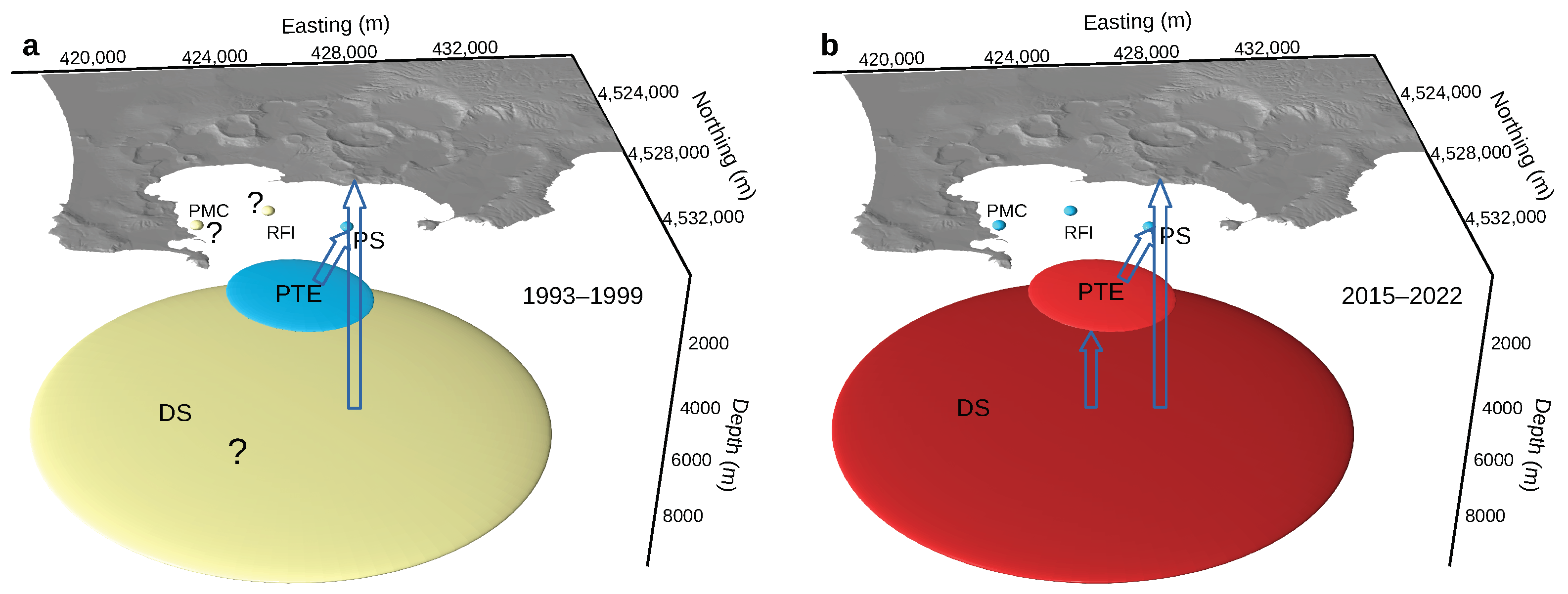Figure 12 summarizes the behavior of the PTE, DS, PS, RFI and PMC during 1993–1999 and 2015–2022.

Differences between the normalized EOFs and the computed cumulated contributions of the tested sources (PTE, DS, PS, RFI and PMC) are probably ascribable in large part to the simple assumptions of the modeling, which is based on circular sills and oblate spheroids embedded in a homogeneous isotropic elastic half-space, with some correction to the computed horizontal-to-vertical displacement ratio so to roughly account at least for rock layering. However, those differences are very similar for the 1993–2000 subsidence and 2015–2022 uplift (Figure 10c,d and Figure 11c,d), thus suggesting persistent local distortion of the deformation field.

The most intriguing result is certainly the evidence of the inflation of a deep (>7 km) reservoir (DS) since 2015. Until now, some indication of the activity of the deep source—identified by seismic data [17]—had been obtained from the geochemical composition of the fumaroles, but no direct evidence of its dynamics has been provided. Two opposite-polarity sources, about 3000 m and 8000 m deep, respectively, were obtained by [28] from SAR images related to 1993–1999 (subsidence) and 2007–2013 (uplift), after inverting the sole vertical displacements for two Mogi pressure sources embedded in a homogeneous half-space. However, as pointed out e.g., by [37], fitting a Mogi pressure source to uplift data only may yield estimates of the source parameters that are not reliable. Reliability of the source parameters is also affected by the use of a homogeneous half-space without any correction for the presence of layered rock heterogeneity, particularly important at Campi Flegrei [30]. We demonstrate that inflation of the deep source is necessary to justify the differences between the 1993–2000 and 2015–2022 deformation fields, and is currently contributing to about 20% of the caldera deformation (Figure 11g,h). As shown in [34], the contribution of a deformation source at about 8 km depth is also necessary to satisfy vertical displacement data during the period (1400–1536) of increasing seismicity and uplift which preceded the Monte Nuovo eruption.

The activity of the deep source is worrying also given the current elevation of Pozzuoli, which can be considered the point of maximum elevation of the caldera and has returned to the levels of 1984. It becomes even more troubling when considering suggestions by [9] to distinguish between pre-eruptive and non-eruptive unrests: according to [9], successive unrests have promoted the accumulation of stress in the crust, the continuation of the current uplift could lead to a notable increase in seismicity, and there is a greater potential for eruption than during previous unrests.

5. Conclusions

We analyze ground displacement from ERS-ENVISAT and Sentinel-1A SAR images to investigate the 1993–2000 subsidence—including the 2000 uplift—and part (2015–2022) of the present unrest at Campi Flegrei caldera, Italy. Space-time fields are decomposed into uncorrelated spatial patterns and associated temporal evolutions by applying the empirical orthogonal function analysis to the displacement time series. We find that the first EOF is able to capture most of the long-lasting deformation history, while the other modes do not seem to bring clear information, as also suggested by the singular values.

Our main results:

• Confirm that most of the deformation is related to the activity of a 3–4 km deep sill-like source (the PTE), which is inflated by magma and/or magmatic fluids during periods of unrest and deflates during periods of subsidence;
• Evidence ongoing deformation linked to local fluid migration in the Solfatara area (the PS);
• Identify persistent deformation features where peculiar fluid migration processes occurred during the 1982–1984 unrest (the RFI and PMC);
• Evidence inflation of the ∼8 km deep reservoir (the DS) at least since 2015.

The last result is particular important and worrisome. Whatever is really happening, the deep source should be carefully monitored from now on, because magma of the next eruption will come from there.

Future work will be devoted to analyze EOF modes other than the first, link the persistent distortions of the deformation field to geological features of the caldera and/or non-modeled source complexity and, mainly, analyze deformation in a larger area, so to improve on detection of the deep source activity and investigate possible interconnected processes in the Neapolitan volcanic area.

References

1. Rosi, M.; Sbrana, A. (Eds.) Phlegrean Fields. Quaderni de “La Ricerca Scientifica”; CNR: Roma, Italy, 1987; Volume 9, p. 175. ISSN 0556-9664. [Google Scholar]
2. Orsi, G.; Civetta, L.; Del Gaudio, C.; de Vita, S.; Di Vito, M.; Isaia, R.; Petrazzuoli, S.; Ricciardi, G.; Ricco, C. Short-term ground deformations and seismicity in the resurgent Campi Flegrei caldera Italy: An example of active block-resurgence in a densely populated area. J. Volcanol. Geotherm. Res. 1999, 91, 415–451. [Google Scholar] [CrossRef]
3. TINITALY, 10 m-Cell Size Grid. Available online: http://tinitaly.pi.ingv.it/Download_Area2.html (accessed on 17 August 2022).
4. De Martino, P.; Dolce, M.; Brandi, G.; Scarpato, G.; Tammaro, U. The Ground Deformation History of the Neapolitan Volcanic Area (Campi Flegrei Caldera, Somma–Vesuvius Volcano, and Ischia Island) from 20 Years of Continuous GPS Observations (2000–2019). Remote Sens. 2021, 13, 2725. [Google Scholar] [CrossRef]
5. Amoruso, A.; Crescentini, L.; Sabbetta, I. Paired deformation sources of the Campi Flegrei caldera (Italy) required by recent (1980–2010) deformation history. J. Geophys. Res. Solid Earth 2014, 119, 858–879. [Google Scholar] [CrossRef]
6. De Siena, L.; Chiodini, G.; Vilardo, G.; Del Pezzo, E.; Castellano, M.; Colombelli, S.; Tisato, N.; Ventura, G. Source and dynamics of a volcanic caldera unrest: Campi Flegrei, 1983–84. Sci. Rep. 2017, 7, 8099. [Google Scholar] [CrossRef] [Green Version]
7. Chiodini, G.; Caliro, S.; Avino, R.; Bini, G.; Giudicepietro, F.; De Cesare, W.; Ricciolino, P.; Aiuppa, A.; Cardellini, C.; Petrillo, Z.; et al. Hydrothermal pressure-temperature control on CO2 emissions and seismicity at Campi Flegrei (Italy). J. Volcanol. Geotherm. Res. 2021, 414, 107245. [Google Scholar] [CrossRef]
8. Buono, G.; Paonita, A.; Pappalardo, L.; Caliro, S.; Tramelli, A.; Chiodini, G. New insights into the recent magma dynamics under Campi Flegrei caldera (Italy) from petrological and geochemical evidence. J. Geophys. Res. Solid Earth 2022, 127, e2021JB023773. [Google Scholar] [CrossRef]
9. Kilburn, C.R.; De Natale, G.; Carlino, S. Progressive approach to eruption at Campi Flegrei caldera in southern Italy. Nat. Commun. 2017, 8, 15312. [Google Scholar] [CrossRef] [Green Version]
10. Amoruso, A.; Crescentini, L.; Berrino, G. Simultaneous inversion of deformation and gravity changes in a horizontally layered half-space: Evidences for magma intrusion during the 1982–1984 unrest at Campi Flegrei caldera (Italy). Earth Planet. Sci. Lett. 2008, 272, 181–188. [Google Scholar] [CrossRef]
11. Castaldo, R.; Tizzani, P.; Solaro, G. Inflating Source Imaging and Stress/Strain Field Analysis at at Campi Flegrei Caldera: The 2009–2013 Unrest Episode. Remote Sens. 2021, 13, 2298. [Google Scholar] [CrossRef]
12. Chiodini, G.; Paonita, A.; Aiuppa, A.; Costa, A.; Caliro, S.; De Martino, P.; Acocella, V.; Vandemeulebrouck, J. Magmas near the critical degassing pressure drive volcanic unrest towards a critical state. Nat. Commun. 2016, 7, 13712. [Google Scholar] [CrossRef]
13. Arienzo, I.; Moretti, R.; Civetta, L.; Orsi, G.; Papale, P. The feeding system of Agnano-Monte Spina eruption (Campi Flegrei, Italy): Dragging the past into present activity and future scenarios. Chem. Geol. 2010, 270, 135–147. [Google Scholar] [CrossRef]
14. Moretti, R.; Arienzo, I.; Civetta, L.; Orsi, G.; Papale, P. Multiple magma degassing sources at an explosive volcano. Earth Planet. Sci. Lett. 2013, 367, 95–104. [Google Scholar] [CrossRef]
15. Amoruso, A.; Crescentini, L.; Sabbetta, I.; De Martino, P.; Obrizzo, F.; Tammaro, U. (Clues to the cause of the 2011–2013 Campi Flegrei caldera unrest, Italy, from continuous GPS data. Geophys. Res. Lett. 2014, 41, 3081–3088. [Google Scholar] [CrossRef]
16. De Siena, L.; Amoruso, A.; Del Pezzo, E.; Wakeford, Z.; Castellano, M.; Crescentini, L. Space-weighted seismic attenuation mapping of the aseismic source of Campi Flegrei 1983–1984 unrest. Geophys. Res. Lett. 2017, 44, 1740–1748. [Google Scholar] [CrossRef] [Green Version]
17. Zollo, A.; Maercklin, N.; Vassallo, M.; Dello Iacono, D.; Virieux, J.; Gasparini, P. Seismic reflections reveal a massive melt layer feeding Campi Flegrei caldera. Geophys. Res. Lett. 2008, 35, L12306. [Google Scholar] [CrossRef] [Green Version]
18. Fedi, M.; Cella, F.; D’Antonio, M.; Florio, G.; Paoletti, V.; Morra, V. Gravity modeling finds a large magma body in the deep crust below the Gulf of Naples, Italy. Sci. Rep. 2018, 8, 8229. [Google Scholar] [CrossRef]
19. Fournier, N.; Chardot, L. Understanding volcano hydrothermal unrest from geodetic observations: Insights from numerical modeling and application to White Island volcano, New Zealand. J. Geophys. Res. 2012, 117, B11208. [Google Scholar] [CrossRef]
20. Envisat Mission Description. Available online: https://earth.esa.int/eogateway/missions/envisat (accessed on 17 August 2022).
21. Sentinel1 Mission Description. Available online: https://sentinel.esa.int/web/sentinel/missions/sentinel-1 (accessed on 17 August 2022).
22. Berardino, P.; Fornaro, G.; Lanari, R.; Sansosti, E. A New Algorithm for Surface Deformation Monitoring Based on Small Baseline Differential SAR Interferograms. IEEE Trans. Geosci. Remote Sens. 2002, 40, 2375–2383. [Google Scholar] [CrossRef] [Green Version]
23. Sentinel-1 Acquisition Modes, Interferometric Wide Swath. Available online: https://sentinels.copernicus.eu/web/sentinel/user-guides/sentinel-1-sar/acquisition-modes/interferometric-wide-swath (accessed on 17 August 2022).
24. Alaska Satellite Facility. Available online: https://asf.alaska.edu/data-sets/sar-data-sets/sentinel-1/ (accessed on 17 August 2022).
25. Sandwell, D.; Mellors, R.; Tong, X.; Wei, M.; Wessel, P. Open radar interferometry software for mapping surface deformation. Eos Trans. AGU 2011, 92, 234–235. [Google Scholar] [CrossRef] [Green Version]
26. Tymofyeyeva, E.; Fialko, Y. Mitigation of atmospheric phase delays in InSAR data, with application to the eastern California shear zone. J. Geophys. Res. Solid Earth 2015, 120, 5952–5963. [Google Scholar] [CrossRef]
27. Navarra, A.; Simoncini, V. A Guide to Empirical Orthogonal Functions for Climate Data Analysis; Springer: Dordrecht, The Netherlands, 2010; p. 151. ISBN 978-90-481-3701-5. [Google Scholar]
28. Tiampo, K.F.; González, P.J.; Samsonov, S.; Fernández, J.; Camacho, A. Principal component analysis of MSBAS DInSAR time series from Campi Flegrei, Italy. J. Volcanol. Geotherm. Res. 2017, 344, 139–153. [Google Scholar] [CrossRef] [Green Version]
29. Amoruso, A.; Crescentini, L.; Fidani, C. Effects of crustal layering on source parameter inversion from coseismic geodetic data. Geophys. J. Int. 2004, 159, 353–364. [Google Scholar] [CrossRef] [Green Version]
30. Crescentini, L.; Amoruso, A. Effects of crustal layering on the inversion of deformation and gravity data in volcanic areas: An application to the Campi Flegrei caldera, Italy. Geophys. Res. Lett. 2007, 34, L09303. [Google Scholar] [CrossRef]
31. Fialko, Y.; Khazan, Y.; Simons, M. Deformation due to a pressurized horizontal circular crack in an elastic half-space, with applications to volcano geodesy. Geophys. J. Int. 2001, 146, 181–190. [Google Scholar] [CrossRef] [Green Version]
32. Battaglia, M.; Cervelli, P.F.; Murray, J.R. dMODELS: A MATLAB software package for modeling crustal deformation near active faults and volcanic centers. J. Volcanol. Geotherm. Res. 2013, 254, 1–4. [Google Scholar] [CrossRef]
33. Cervelli, P.F. Analytical expressions for deformation from an arbitrarily oriented spheroid in a half-space. In Proceedings of the American Geophysical Union Fall Meeting, San Francisco, CA, USA, 9–13 December 2013. [Google Scholar]
34. Amoruso, A.; Crescentini, L.; D’Antonio, M.; Acocella, V. Thermally-assisted magma emplacement explains restless calderas. Sci. Rep. 2017, 7, 7948. [Google Scholar] [CrossRef] [Green Version]
35. Cigna, F.; Esquivel Ramírez, R.; Tapete, D. Accuracy of Sentinel-1 PSI and SBAS InSAR Displacement Velocities against GNSS and Geodetic Leveling Monitoring Data. Remote Sens. 2021, 13, 4800. [Google Scholar] [CrossRef]
36. Giudicepietro, F.; Chiodini, G.; Avino, R.; Brandi, G.; Caliro, S.; De Cesare, W.; Galluzzo, D.; Esposito, A.; La Rocca, A.; Lo Bascio, D.; et al. Tracking Episodes of Seismicity and Gas Transport in Campi Flegrei Caldera Through Seismic, Geophysical, and Geochemical Measurements. Seismol. Res. Lett. 2021, 92, 965–975. [Google Scholar] [CrossRef]
37. Battaglia, M.; Segall, P. The Interpretation of Gravity Changes and Crustal Deformation in Active Volcanic Areas. Pure Appl. Geophys. 2004, 161, 1453–1467. [Google Scholar] [CrossRef]
Figure 1. Map of the Campi Flegrei caldera, UTM WGS84 33N coordinates. Colors give topography [3]. Cyan and light blue discontinuous lines with triangles indicate the Campanian Ignimbrite (CI) and Neapolitan Yellow Tuff (NYT) caldera borders, respectively (adapted from [2]). Magenta labels and dots: M, Mofete area; MN, Monte Nuovo; P, Pozzuoli; SF, Solfatara fumarolic field. Red labels and circles: 25A, leveling benchmark in the area of maximum vertical displacement; LR, reference benchmark for levelings. Black labels and dots: continuous GPS stations [4] used to validate Sentinel 1A displacement time series; GPS and SAR displacements are referred to MAFE for validation. Blue labels and triangles: PS, injection point of magmatic fluids into the hydrothermal system [5]; RFI, area of repeated fluid injections during 1983–1984 [6]; PMC, area of the fluid transfer connection between Pozzuoli and Mofete/Monte Nuovo where the spatial 1983–1984 seismic pattern turns from E-W to NW-SE [6]; DS, center of the deep reservoir contributing to 2015–2022 deformation. Blue label and dashed ellipse: PTE, border of the around 3500 m deep sill-like reservoir [5]. The black dashed circle bounds the area where EOFs of SAR displacements are computed.
Remotesensing 14 05698 g001
Figure 2. Ground level changes in the area of maximum vertical displacement. Blue dots, leveling data [5] at benchmark 25A referred to LR (see Figure 1). Red crosses and pluses, median vertical displacement referred to LR inside a 200 m radius circular area around benchmark 25A from ERS/ENVISAT and Sentinel-1A images, respectively. Green dots, GPS vertical displacement of RITE referred to a net of six stations of the INGV RING (Rete Integrata Nazionale GNSS) network located outside the Neapolitan volcanic area [4]. Cyan bars indicate the two time periods—1993–2000 and 2015–2022—investigated in this work.
Remotesensing 14 05698 g002
Figure 3. Time series of SAR LOS displacements. (a) Red and green squares, acquisition dates of the ascending- and descending-orbit images; only those out of the grey rectangle are used in this work. (b) Mean LOS displacement rate during 1993–1999, ERS/ENVISAT ascending orbit. (c) Mean LOS displacement rate during 2015–2022, Sentinel-1A ascending orbit. (d) Mean LOS displacement rate during 1993–1999, ERS/ENVISAT descending orbit. (e) Mean LOS displacement rate during 2015–2022, Sentinel-1A descending orbit.
Remotesensing 14 05698 g003
Figure 4. Time series of SAR vertical and horizontal displacements. (a) Dates of vertical and horizontal displacement data used in this work. (b) Mean upward displacement rate during 1993–1999, ERS/ENVISAT. (c) Mean upward displacement rate during 2015–2022, Sentinel-1A. (d) Mean eastward displacement rate during 1993–1999, ERS/ENVISAT. (e) Mean eastward displacement rate during 2015–2022, Sentinel-1A.
Remotesensing 14 05698 g004
Figure 5. Comparison between GPS and Sentinel-1A SAR vertical and eastward displacements for the GPS stations within the dashed black circle in Figure 1. GPS displacements (black dots) are referred to MAFE (see Figure 1); SAR displacements (red dots) are referred to the median value within a circular area, 200 m in radius, centered on MAFE.
Remotesensing 14 05698 g005
Figure 6. Temporal evolutions and singular values for the first modes from the joint EOF analysis of vertical and eastward displacements: (a) temporal evolutions from ERS/ENVISAT data; (b) temporal evolutions from Sentinel-1A data; (c) singular values from ERS/ENVISAT data; (d) singular values from Sentinel-1A data. The y-axis scales in (a,b) are arbitrary because the temporal evolution has to be multiplied by the related vertical and eastward displacement EOF coefficient of each pixel to obtain displacement time histories.
Remotesensing 14 05698 g006
Figure 7. Spatial patterns of the first mode from the joint EOF analysis of vertical and eastward displacements. Vertical and eastward EOFs are normalized by the range of variability (difference of the maximum and minimum values) of the vertical EOF for each time period (1993–2000 and 2015–2022), see Section 2.4. (a) ERS/ENVISAT data, vertical displacement ( h ˜ 1 v in Equation (2)); (b) ERS/ENVISAT data, eastward displacement ( h ˜ 1 e in Equation (2)); (c) Sentinel-1A data, vertical displacement ( h ˜ 2 v in Equation (2)); (d) Sentinel-1A data, eastward displacement ( h ˜ 2 e in Equation (2)); (e) difference of values in (a,c) ( h ˜ 1 v h ˜ 2 v in Equation (3)); (f) difference of values in (b,d) ( h ˜ 1 e h ˜ 2 e in Equation (3)). Green and magenta triangles and labels in panels (e,f) correspond to the positions of the DS, PMC, RFI and PS. Color palette and range in (e,f) have been chosen so to enhance visibility of the pattern differences between 1993–2000 and 2015–2022.
Remotesensing 14 05698 g007
Figure 8. Modeling of the differences between the 1993–2000 and 2015–2022 normalized EOFs. (a,b) Difference between normalized EOFs ( h ˜ 1 v h ˜ 2 v and h ˜ 1 e h ˜ 2 e in Equation (3), respectively), redrawn from Figure 7e,f for clarity. (c,d) Computed cumulative contribution of the PS, RFI, PMC, PTE and DS deformation sources to the difference between normalized EOFs, i.e., k = 1 5 a 1 , k / r 1 v a 2 , k / r 2 v f k v and k = 1 5 a 1 , k / r 1 v a 2 , k / r 2 v f k e in Equation (3), respectively. (e,f) Model residuals, i.e., differences of the left and right side of Equation (3).
Remotesensing 14 05698 g008
Figure 9. Contribution of each deformation source to the differences between the 1993–2000 and 2015–2022 normalized EOFs. Maps show a 1 , k / r 1 v a 2 , k / r 2 v f k v and a 1 , k / r 1 v a 2 , k / r 2 v f k e in Equation (3), where subscript k indicates the deformation source. (a), PTE, vertical displacement; (b), PTE, eastward displacement; (c), DS, vertical displacement; (d), DS, eastward displacement; (e), PS, vertical displacement; (f), PS, eastward displacement; (g), RFI, vertical displacement; (h), RFI, eastward displacement; (i), PMC, vertical displacement; (j), PMC, eastward displacement. The green or magenta dot in each panel gives the center position of the related source.
Remotesensing 14 05698 g009
Figure 10. Modeling of the normalized 1993–2000 EOFs. (a,b) Normalized vertical and horizontal EOFs ( h ˜ 1 v and h ˜ 1 e in Equation (2), respectively), redrawn from Figure 7a,b. (c,d) Model residuals after subtracting the cumulative contribution of the PTE, DS, PS, RFI and PMC. (e,f) Contribution of the PTE, i.e., a 1 , 1 / r 1 v f 1 v and a 1 , 1 / r 1 v f 1 e in Equation (2), respectively. (g,h) Contribution of the DS, i.e., a 1 , 2 / r 1 v f 2 v and a 1 , 2 / r 1 v f 2 e in Equation (2), respectively. The magenta dot in panels (eh) gives the center position of the related source.
Remotesensing 14 05698 g010
Figure 11. Modeling of the normalized 2015–2022 EOFs. (a,b) Normalized vertical and horizontal EOFs ( h ˜ 2 v and h ˜ 2 e in Equation (2), respectively), redrawn from Figure 7a,b. (c,d) Residuals after subtracting the cumulative contribution of the PTE, DS, PS, RFI and PMC. (e,f) Contribution of the PTE, i.e., a 2 , 1 / r 2 v f 1 v and a 2 , 1 / r 2 v f 1 e in Equation (2), respectively. (g,h) Contribution of the DS, i.e., a 2 , 2 / r 2 v f 2 v and a 2 , 2 / r 2 v f 2 e in Equation (2), respectively. The magenta dot in panels (eh) gives the center position of the related source.
Remotesensing 14 05698 g011
Figure 12. Cartoons of the dynamics of the PTE, DS, PS, RFI and PMC deformation sources in different periods. (a), 1993–1999; (b), 2015–2022. The time period in (a) is 1993–1999 instead of 1993–2000 (as from 1993-2000 SAR data) to exclude the 2000 mini-uplift (see Figure 2). Reddish colors indicate source inflation, cyan indicates deflation and yellow indicates lack of reliable detected activity, emphasized by question marks. Empty blue arrows schematize possible magmatic fluid transfers from the DS and PTE.
Remotesensing 14 05698 g012