Article

Prediction of Future Spatial and Temporal Evolution Trends of Reference Evapotranspiration in the Yellow River Basin, China

1
Yellow River Laboratory, Zhengzhou University, Zhengzhou 450001, China
2
China Institute of Water Resources and Hydropower Research, Beijing 100038, China
*
Author to whom correspondence should be addressed.
Remote Sens. 2022, 14(22), 5674; https://doi.org/10.3390/rs14225674
Submission received: 15 October 2022 / Revised: 6 November 2022 / Accepted: 7 November 2022 / Published: 10 November 2022
(This article belongs to the Topic Water Management in the Era of Climatic Change)

Abstract

:
Reference evapotranspiration (ET0) is an integral part of the regional hydrological cycle and energy balance and is extremely sensitive to climate change. Based on temperature data from 24 global climate models (GCMs) in the Coupled Model Intercomparison Project Phase 6 (CMIP6), this study developed a multi-model ensemble based on delta statistical downscaling with multiple interpolation methods and evaluation indicators to predict the spatial and temporal evolution trends of ET0 in the Yellow River Basin (YRB) under four emission scenarios (SSP126, SSP245, SSP370, and SSP585) for the near- (2022–2040), mid- (2041–2060), and long- (2081–2100) term future. Results demonstrate that regional data generated based on delta statistical downscaling had good simulation performance for the monthly mean, maximum, and minimum temperatures in the YRB, and the developed multi-model ensemble had better simulation capability than any single model. Compared to the historical period (1901–2014), the annual ET0 showed a highly significant increase for different future emission scenarios, and the increase is faster with increasing radiative forcing. The first main cycle of ET0 change was 52, 53, 60, and 48 years for the SSP126, SSP245, SSP370, and SSP585, respectively. ET0 in the YRB had positive values for EOF1 under all four emission scenarios, responding to a spatially consistent trend across the region. Compared to the historical period, the spatial distribution of ET0 under different future emission scenarios was characterized by being larger in the west and smaller in the east. As the radiative forcing scenario increased and time extended, ET0 significantly increased, with a maximum variation of 112.91% occurring in the western part of the YRB in the long-term future under the SSP585 scenario. This study can provide insight into the water cycle patterns of watersheds and scientific decision support for relevant departments to address the challenges of climate change.

1. Introduction

Climate change and its impacts on the water cycle, particularly on regional hydrological systems, are major global challenges in the 21st century [1,2,3]. As an important factor in the regional hydrological cycle and energy balance, reference evapotranspiration (ET0) can be used to make total energy estimates of actual evapotranspiration [4], and is the component of the water cycle that is directly affected by climate change. Changes in ET0 have a significant impact on the global water cycle and water resources [5], thereby leading to droughts and floods, water scarcity, and ecosystem degradation. In the context of climate change, ET0 is an important guide for understanding the hydrological cycle and formulating water resource plans in watersheds [6,7,8].
Although studies on ET0 have been conducted recently [9,10,11,12,13,14], most existing studies focused on the historical period. With the development of global climate models (GCMs), exploring the future ET0 of watersheds based on historical data has become a topic of research interest in the context of climate change. GCMs are the most powerful tools for climate change modeling and future predictions [15,16], and the modeling results can provide valuable data to support studies on climate change-induced impacts at regional and continental scales. Nevertheless, low-resolution data will lead to large biases in the prediction of regional climate change when climate studies are conducted at regional scales. Downscaling is an effective method for transforming large-scale, low-resolution outputs from GCMs into small-scale, high-resolution regional ground information [17,18]. Current mainstream downscaling methods include dynamic downscaling [19] and statistical downscaling [20]. Compared to statistical downscaling, dynamic downscaling requires a large number of complex inputs and computational requirements [21,22], and sometimes fine and reliable climate data at regional scales are not available [22,23]. Statistical downscaling is the most widely used and established downscaling technique in basin climate change studies because of its low computational cost, easy model construction, multiple implementation methods, ease of operation, and lack of consideration of the influence of boundary conditions on prediction results [24].
Two methods are widely used for ET0 prediction under future climate scenarios: (1) input of future meteorological data from GCMs into ET0 models [25,26]; and (2) directly predicting future ET0 via downscaling methods based on historical ET0 [1,27]. Liu et al. [28] used Coupled Model Intercomparison Project Phase 5 (CMIP5) and Coupled Model Intercomparison Project Phase 6 (CMIP6) climate models to compare global potential evapotranspiration and found that both models could effectively simulate the increasing trend; they also revealed that CMIP6 multi-model results simulated higher values of global potential evapotranspiration than CMIP5 for the same emission scenario. Nistor et al. [29] assessed the impact of climate change on ET0 in Turkey in the 21st century based on the Thornthwaite equation and the CMIP5 dataset. They revealed that ET0 will increase in southern and southeastern Turkey and along the Mediterranean coast in the coming period owing to climate warming.
The Yellow River Basin (YRB) is an important component of China’s strategic ecological security pattern, and most of the YRB is an arid and semi-arid region. Because of its unique geographical location, its environment is fragile and highly sensitive to global climate change [21,30], making it a good indicator of climate change. Despite the high sensitivity of the region to climate change, studies on the evolution of ET0 in the YRB in the context of future climate are limited, and most of the existing studies on future ET0 in other regions are at the CMIP5 stage [21,30,31], with no downscaling treatment [1], a single spatial interpolation method [21], or a single indicator for climate model preferences [32]. Therefore, against the backdrop of global warming, the ET0 predictions in the YRB can provide a theoretical reference basis for water resource planning and management, as well as a scientific basis for relevant authorities to formulate future climate change response strategies.
This study used the YRB as the study area and developed a multi-model ensemble based on the delta statistical downscaling using multiple interpolation methods and multiple evaluation indicators to predict the spatial and temporal evolution characteristics of ET0 in the YRB under different CMIP6 emission scenarios. Studies on ET0 not only enhance the understanding of hydrological processes in the YRB but also provide data to support and guide future water resource management and drought mitigation. The specific objectives are to: (1) obtain monthly mean, maximum, and minimum temperature datasets in the YRB with a resolution of 1 × 1 km based on CMIP6 climate model data and delta statistical downscaling; (2) select the best simulated climate model and multi-model ensemble by evaluating and validating historical measured data; and (3) predict the spatial and temporal changes in ET0 under different emission scenarios in the future based on the Hargreaves formula and downscaled temperature data from 2022 to 2100.

2. Materials and Methods
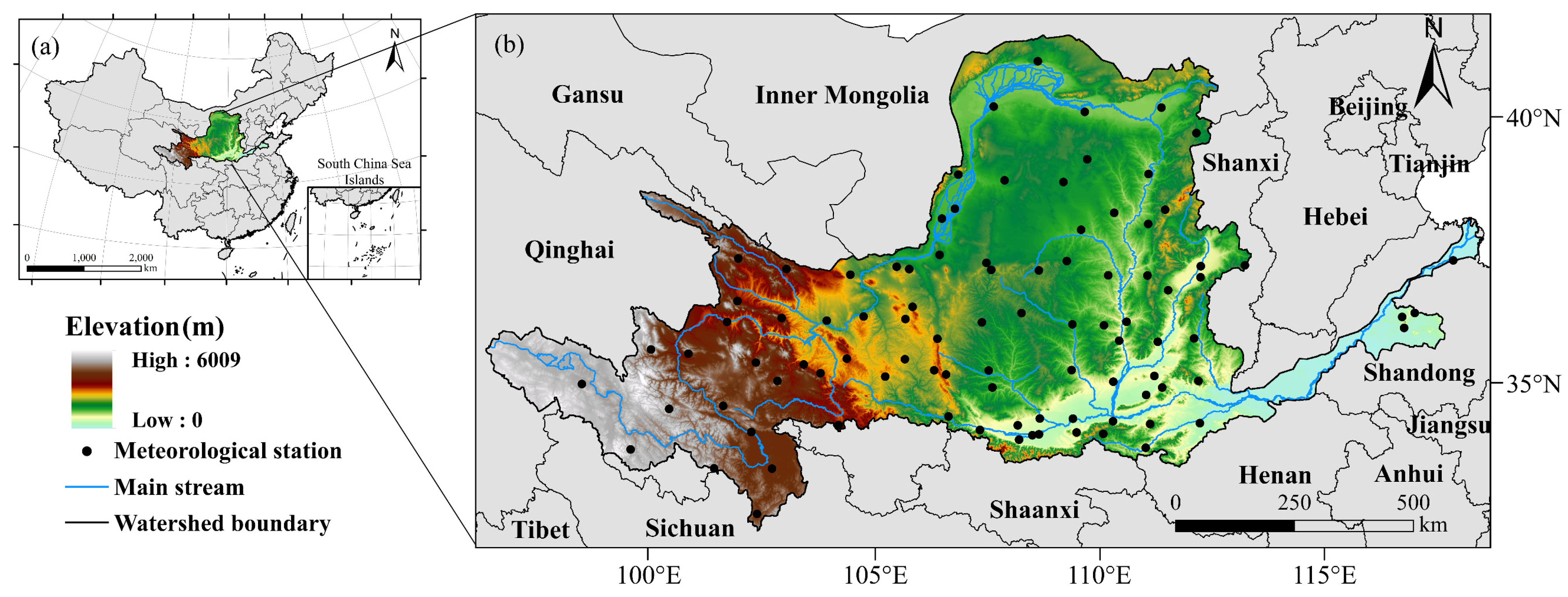
2.1. Study Area

The Yellow River, the second-largest river in China, starts from the Bayankara Mountains in the west, crosses the Qinghai–Tibetan Plateau, Loess Plateau, and Huang-Huai-Hai Plain, and flows into the Bohai Sea in Shandong Province. The total length of the basin is 5464 km, covering an area of approximately 79.5 × 10⁴ km2 (95°53′E–119°05′E, 32°10′N–41°50′N), accounting for 8% of China’s land area (Figure 1). The YRB is in the mid-latitude zone, with complex natural conditions and undulating basin topography, and is influenced by atmospheric and monsoonal circulation, making the climate different from that of the other basins in China [33,34]. The average annual precipitation in the basin is 495 mm, with concentrated and highly variable interannual precipitation and an evident downward trend from the southeast to the northwest [35]. The average annual temperature ranges from −4 to 14 °C, varying with latitude and altitude [36]. The basin’s evapotranspiration varies markedly, with an average annual ET0 of 700–1800 mm and an increasing trend from the southeast to the northwest. As the basin straddles arid, semi-arid, and semi-humid zones, it is in the transition zone between semi-arid and semi-humid climates, rendering it extremely sensitive to climate change [21]. Climate change has exacerbated the uneven spatial and temporal distributions of water resources in the YRB, and the contradiction between water resource supply and demand has become evident, seriously affecting the production and life of human society and restricting the high-quality economic development of the region.

2.2. Data Collection

2.2.1. Ground-Based Observation Data

In this study, monthly monitoring data from 93 national meteorological stations in the YRB from 1980 to 2014 were obtained from the National Meteorological Information Centre-China Meteorological Data Network (http://data.cma.cn/ (accessed on 11 March 2022)), including monthly mean temperature (tas), monthly mean maximum temperature (tasmax), monthly mean minimum temperature (tasmin), and monthly pan evaporation. Some of the missing data were reasonably interpolated via the hydrologic analogy method and the linear interpolation method. The tas, tasmax, and tasmin were used to assess the accuracy of the climate model simulations, and the converted value based on pan evaporation data [4] were used to assess the ET0 values based on the multi-model ensemble and Hargreaves formula.

2.2.2. Reference Data on Downscaling

The national 30-year cumulative mean, mean maximum, and mean minimum temperature datasets with a resolution of 1 km from 1971 to 2000 were selected as the regional high-resolution reference data to construct the delta statistical downscaling model in this study. Data were obtained from the National Ecosystem Science Data Center (NESDC) (http://www.nesdc.org.cn/ (accessed on 9 May 2022)).

2.2.3. Future Climate Data

In this study, 24 GCMs were selected from CMIP6 (https://esgf-node.llnl.gov/search/cmip6/ (accessed on 13 May 2022)) for the historical period (1901–2014) and three future periods (near-term 2022–2040, mid-term 2041–2060, and long-term 2081–2100). The tas, tasmax, and tasmin data of the models were presented, which contained 21, 19, and 21 GCMs, respectively; the basic details about each model and variable are summarized in Table 1. For future forcing scenarios, the recent shared socioeconomic pathways (SSPs), such as SSP1-2.6 (low-forcing scenario, SSP126), SSP2-4.5 (medium-forcing scenario, SSP245), SSP3-7.0 (medium to high-forcing scenario, SSP370), and SSP5-8.5 (high-forcing scenario, SSP585), were selected [37]. Notably, the future scenarios of the climate model were set for the 2015–2100 period; the historical period in this study did not extend back to 2021, and the future period did not extend forward to 2015 to ensure the reasonability of the data. The selection of the periods for downscaling the simulation accuracy and Hargreaves model validation were based on these considerations.

2.3. Research Methodology

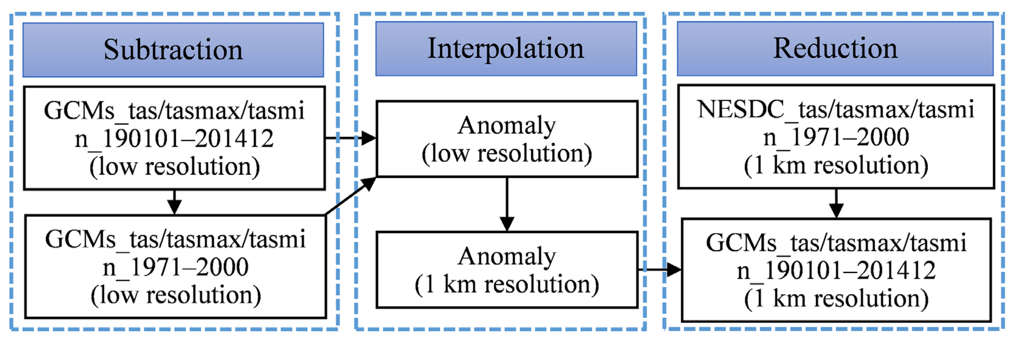
2.3.1. Delta Statistical Downscaling

The delta statistical downscaling method is a simple bias correction technique recommended by the U.S. Global Change Research Program (see http://www.nacc.usgcrp.gov (accessed on 6 June 2022)) that is easy to understand and operate, requires fewer factors, and is widely used in a wide range of fields related to climate change impact studies [21,38,39]. For the temperature variables used in this study, the delta method was used to compare the temperature of different periods of each simulation grid with the simulated average temperature of the base period, calculate the absolute change in temperature in each period of each simulation grid, and add the measured average temperature of each base period with the change in the grid based on the spatial interpolation of the change to obtain the temperature scenarios of different periods in the reconstruction grid [21]. The calculation equation is as follows:
T f = T 0 + ( T M f T M 0 )
where T f is the grid temperature data reconstructed by the delta method, T M f is the simulated grid temperature data for a certain period, T M 0 is the simulated grid multi-year average temperature data for the base period, and T 0 is the measured multi-year average temperature data for the base period. In this study, five interpolation methods were considered: bilinear interpolation (BI), inverse distance weighted (IDW), kriging, natural neighbor interpolation (NNI), and spline. The delta statistical downscaling process is shown in Figure 2.

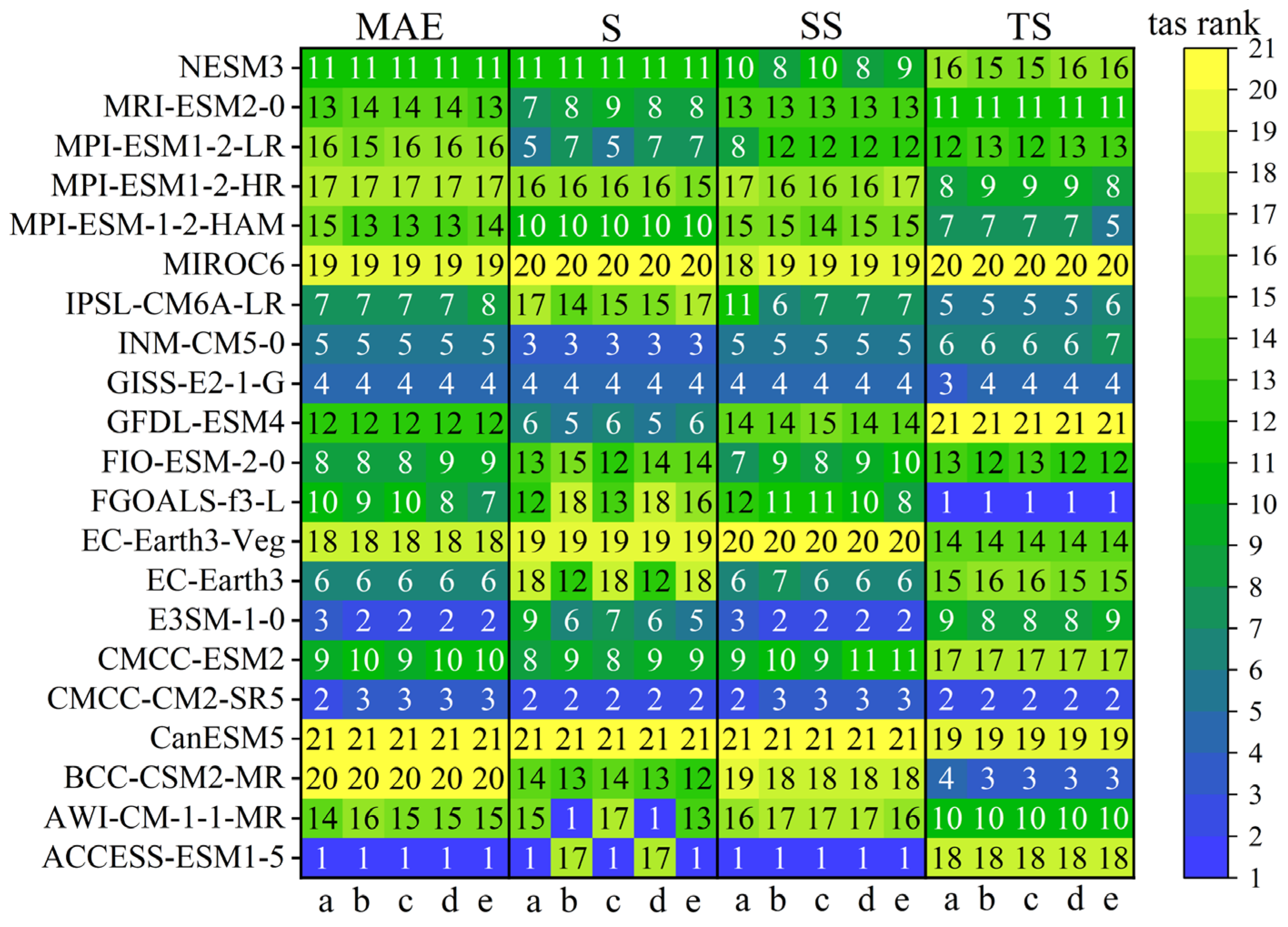
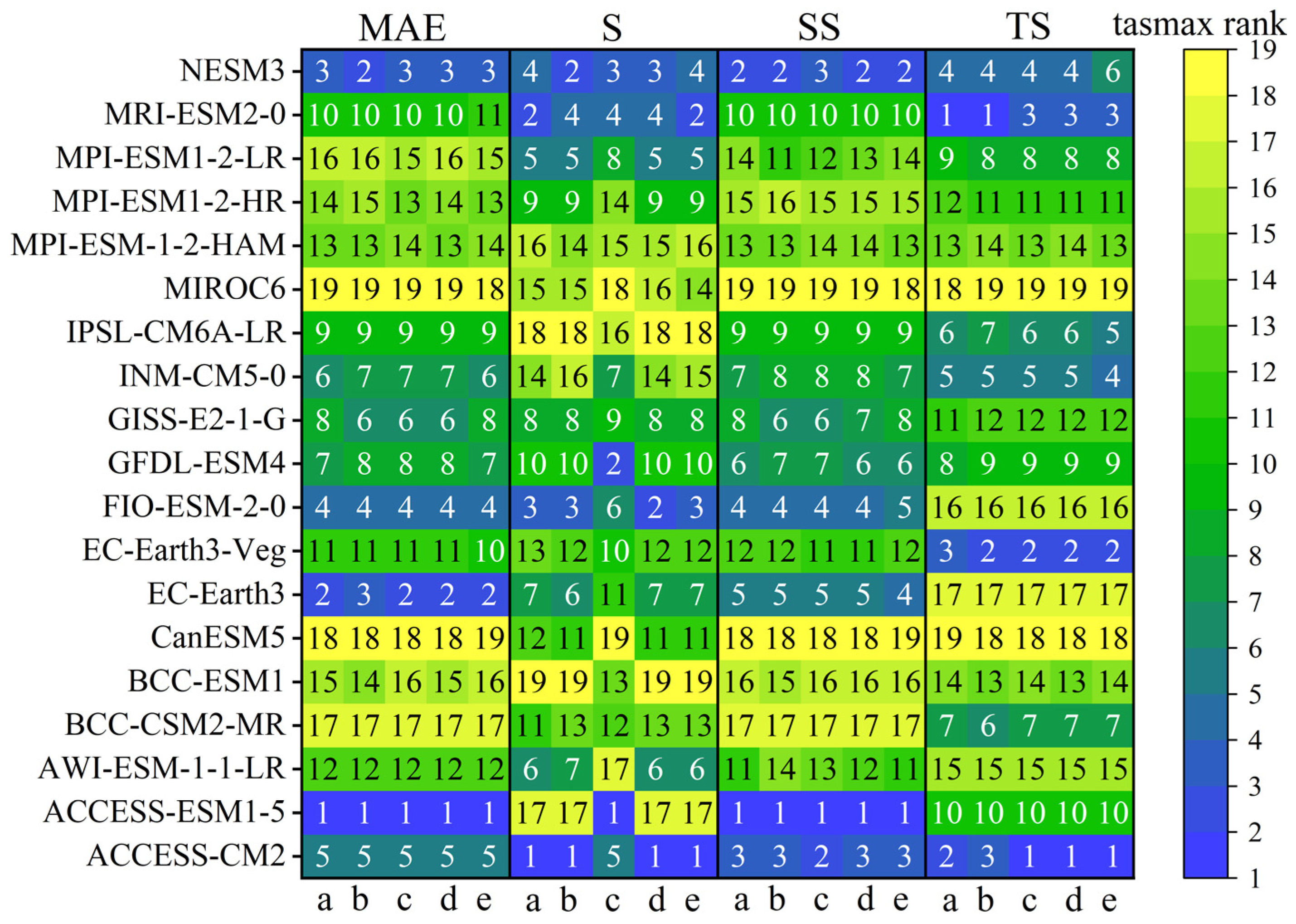
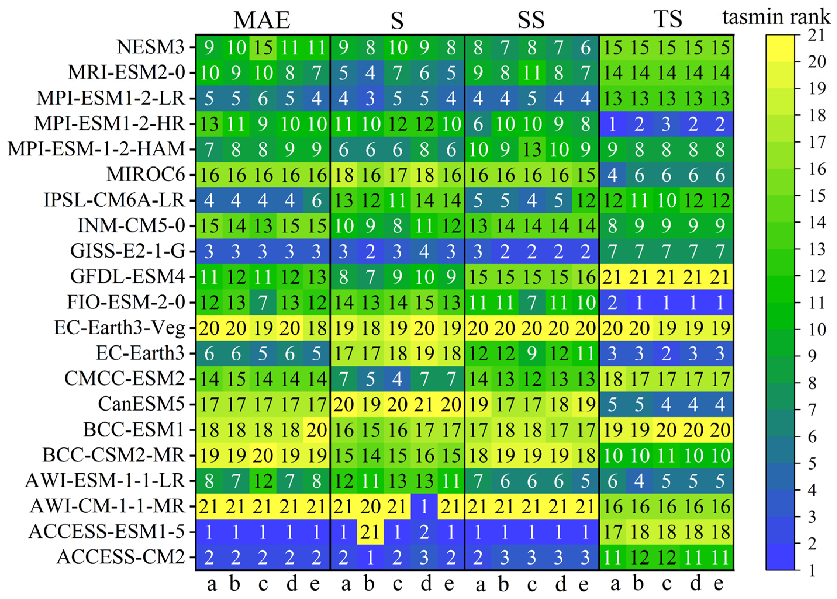
2.3.2. Climate Model Accuracy Assessment and Multi-Model Ensemble

To effectively assess the accuracy and applicability of climate model forecasts in the YRB, the evaluation metrics used were mean absolute error (MAE) [40], Taylor diagram-based quantile S [41], spatial skills score (SS) [42], and temporal skills score (TS) [43]. The closer the MAE and TS are to 0, the better the simulation ability of the model. The closer S and SS are to 1, the better the simulation ability of the model.
The downscaling results of different GCMs differ, and the performance of multi-model averaging is considered to be better than that of individual models [44,45]. In this study, multi-model ensemble averaging of preferred climate models was performed using the equally weighted ensemble averaging (MME) method commonly used in multi-model prediction studies.

2.3.3. ET0 Calculation Model

The Hargreaves model, which can reveal the physics of the evaporative process, was used for calculating monthly ET0 based on a future climate. It has been widely demonstrated to be able to provide reliable estimations [31,46,47]. The Food and Agriculture Organization of the United Nations (FAO) [4] also suggests it as the simplified standard algorithm for ET0 under the missing meteorological observations as required by the Penman–Monteith formula. Several improvements were made to the original equation [48,49]. The form used in this study was published in 1985 [50] and expressed as follows:
E T 0 ( H a r ) = 0.0023 R a ( T m a x T m i n ) 0.5 ( T m e a n + 17.8 )
where E T 0 ( H a r ) is the ET0 calculated by the Hargreaves empirical formula (mm/d); T m a x and T m i n are the mean maximum and minimum temperatures for the calculation time interval (°C), respectively; T m e a n is the mean temperature for the calculation time interval (°C); and R a is the zenith radiation (mm/d); the applicable time scale is 30 or 10 days.

2.3.4. Methods for Spatial and Temporal Trend Analysis

In this study, Morlet wavelet analysis was used to study the significant cycle changes in ET0 time series at different time scales, which has significant advantages in revealing the multiscale configuration and main climate change cycle [51]. Empirical orthogonal function (EOF) analysis produces a set of orthogonal spatial and temporal patterns in the order of explained variance, reducing the dimensionality of the analyzed system and finding relatively few independent variables that can provide comprehensive information about the variability of the raw data [52]. EOF analysis, supplemented by the North test [53], was used to study the spatial and temporal patterns of the ET0 climate field in the YRB. In addition, spatial changes in the near-, mid-, and long-term future relative to the historical period were estimated by comparing historical long-term (1901–2014) annual ET0 averages for different emission scenarios of ET0.

3. Results

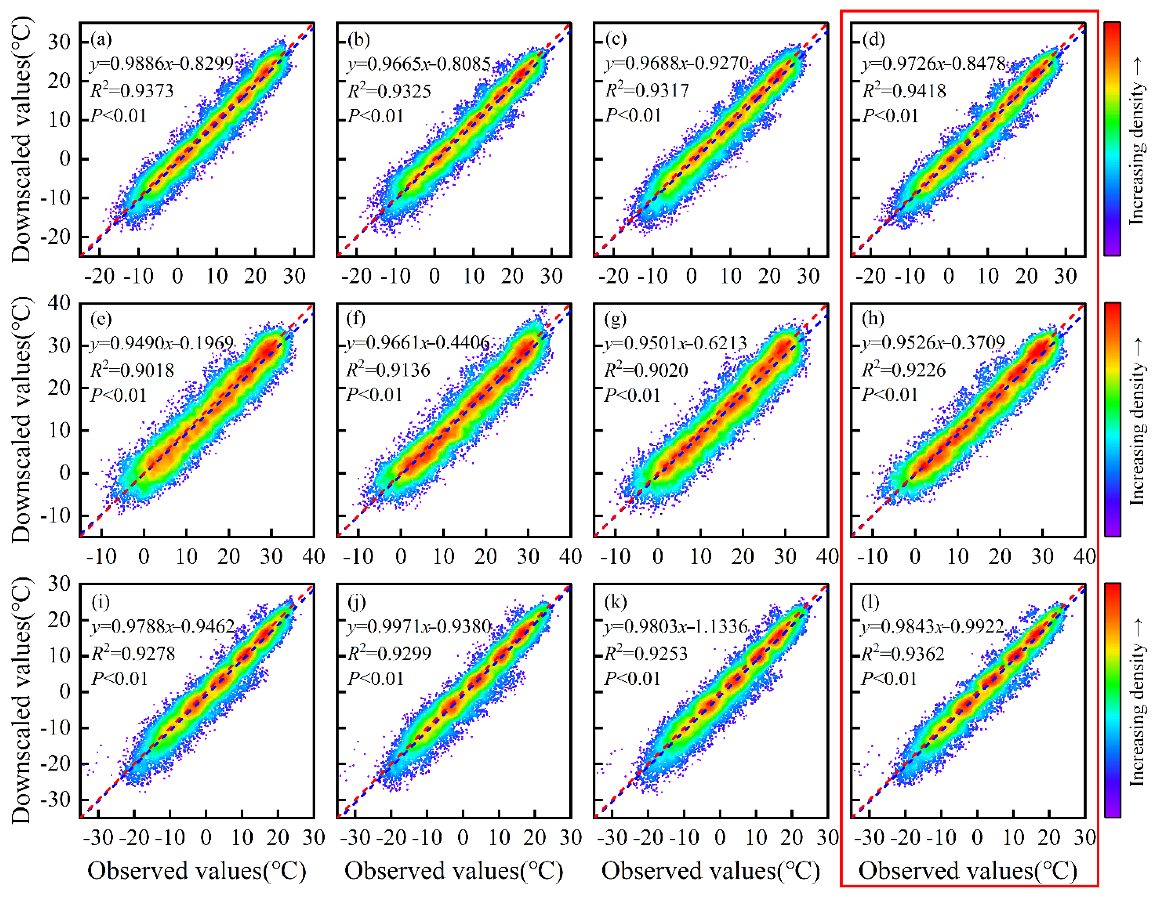
3.1. Simulation Accuracy Assessment of Regional Temperatures and Multi-Model Ensemble

For the three temperature variables, tas, tasmax, and tasmin, out of all interpolation methods, IDW exhibited the lowest overall error for all four different evaluation metrics, and therefore, it was used to further assess the effectiveness of the temperature simulations for all climate models (Figure 3, Figure 4 and Figure 5). For tas, the climate models ACCESS-ESM1-5, CMCC-CM2-SR5, and GISS-E2-1-G were ranked high for each evaluation index; for tasmax, ACCESS-CM2, NESM3, and ACCESS-ESM1-5 were ranked high for each evaluation index; for tasmin, ACCESS-CM2, ACCESS-ESM1-5, and GISS-E2-1-G were ranked high for each evaluation index. Because some climate models do not have data on future emission scenarios, considering the data integrity and actual fitting performance of climate models, tas selected ACCESS-ESM1-5, CMCC-CM2-SR5, and INM-CM5-0; tasmax selected ACCESS-CM2, ACCESS-ESM1-5, and MRI-ESM2-0; and tasmin selected ACCESS-CM2, ACCESS-ESM1-5, and MPI-ESM1-2-LR for the ensemble analysis of subsequent temperature patterns in the YRB. The fitting results of the simulated data of the selected climate model for each variable and MME of the 1995–2014 period to the observed data from 93 ground-based meteorological stations (Figure 6) show that, although the simulated tas, tasmax, and tasmin of the YRB by CMIP6 were slightly lower than the observed values, most of the points were near the 1:1 line, and the R2 and regression coefficients were greater than 0.9, with all passing the 99% confidence level test. The simulated and observed values of the MME dataset were more concentrated than those of the three independent climate models, and the R2 values of the three variables were 0.9418, 0.9226, and 0.9362, respectively (Figure 6d,h,l), which reduced the errors caused by outlier points and slightly improved the fit of the simulated data. The above analysis reveals that climate models have high application potential in the YRB, and the CMIP6 multi-model ensemble is a good reference value for predicting ET0 trends in the YRB under future climate scenarios.

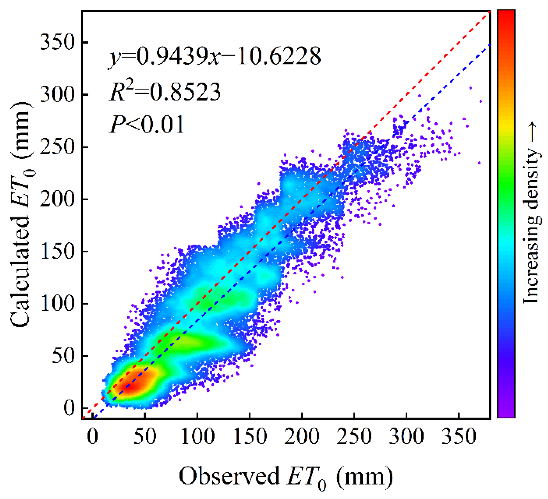
3.2. Simulation Accuracy Assessment of Regional ET0

The scatter density plots of the actual monthly pan evaporation converted values (ET0(pan)) and simulated ET0 values based on the multi-model ensemble-Hargreaves formula (ET0(Har)) for the YRB from 1980 to 2014 (Figure 7) showed that the CMIP6-simulated ET0(Har) for the YRB correlated well with the evaporation dish converted ET0(pan) at the monthly scale, with a fitted line regression coefficient of 0.9439 and R2 of 0.8523, passing the 99% confidence level test. Although the Hargreaves formula partially underestimated ET0, most of the points were near the 1:1 line, making them good reference values for calculating the monthly ET0 under the conditions of missing meteorological observations in the future. Therefore, future ET0 can be simulated using the Hargreaves formula.

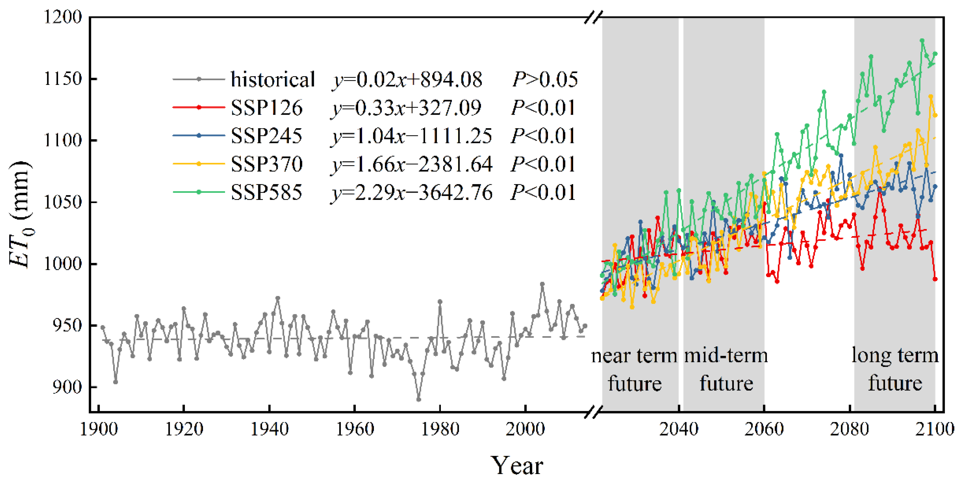
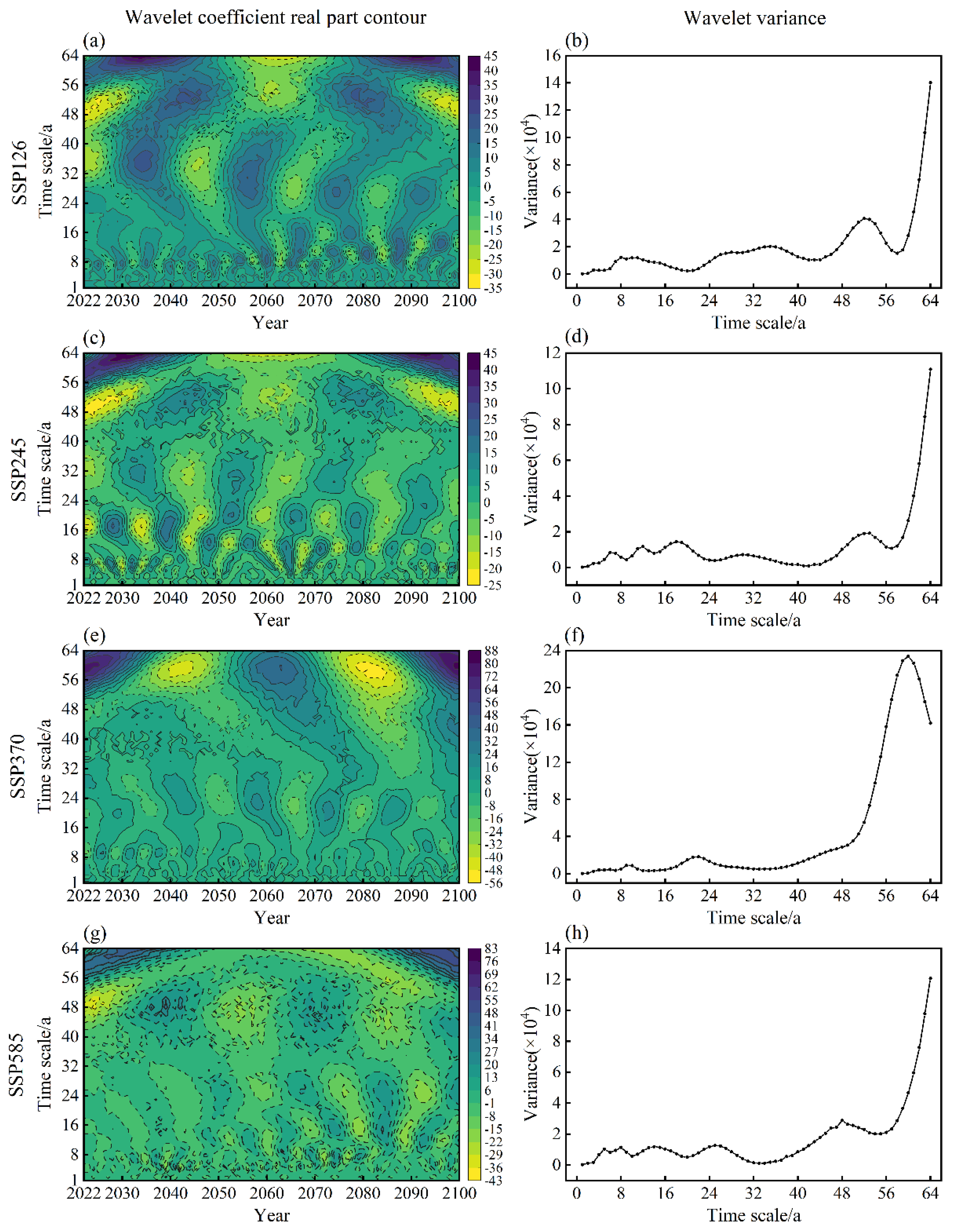
3.3. Temporal Trends and Cyclic Characteristics of ET0

Based on the 1 km high-resolution regional climate data generated by the delta statistical downscaling and multi-model ensemble, annual ET0 trends were estimated for the YRB from 1901 to 2100 (Figure 8). The annual ET0 of the basin under the different future emission scenarios (2022–2100; SSP126, SSP245, SSP370, and SSP585) substantially increased with time relative to the historical period (1901–2014), and all passed the 99% confidence test. Among all scenarios, the SSP585 scenario had the most pronounced upward trend in ET0, increasing at a rate of 22.9 mm/10a, reaching 1170.39 mm in 2100. It was followed by the SSP370 scenario, which increased at a rate of 16.6 mm/10a, reaching 1120.42 mm in 2100. However, SSP245 and SSP126 scenarios had relatively small trends in ET0, increasing at rates of 10.4 and 3.3 mm/10a, reaching 1062.71 and 987.68 mm in 2100, respectively. In general, the annual ET0 in the YRB will rapidly increase with increasing levels of radiative forcing in the future.
To comprehensively understand the temporal ET0 variations in the basin, Morlet wavelet analysis was used to investigate the cyclic variations in ET0 in the YRB under the four future emission scenarios (Figure 9). In the SSP126 scenario, three distinct peaks were observed in the wavelet variance of ET0 in the YRB, corresponding to the time scales of 52, 35, and 8 years, with the most pronounced periodic oscillation of approximately 52 years and a cyclic pattern of 34–38 years for ET0 in the basin under this time scale (Figure 9a,b). In the SSP245 scenario, the ET0 in the YRB considerably oscillated for approximately 53 years, and there was a cyclic pattern of approximately 34 years in the basin ET0 at this time scale (Figure 9c,d). In the SSP370 scenario, the ET0 in the YRB considerably oscillated for approximately 60 years, and there was a cyclic pattern of approximately 39 years in the basin ET0 at this time scale (Figure 9e,f). In the SSP585 scenario, the ET0 in the YRB substantially oscillated for approximately 48 years, and there was a cyclic pattern of approximately 27–32 years in the basin ET0 at this time scale (Figure 9g,h).

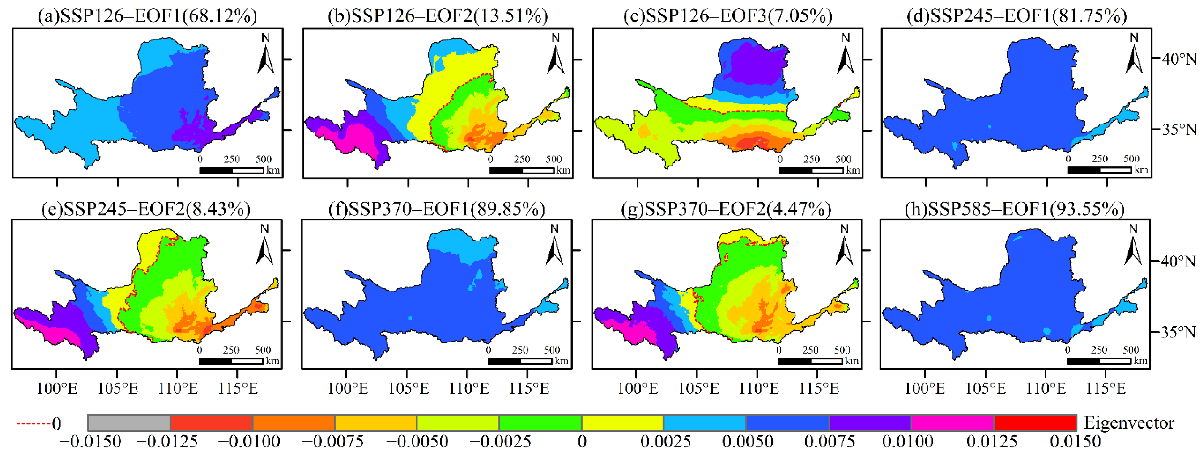
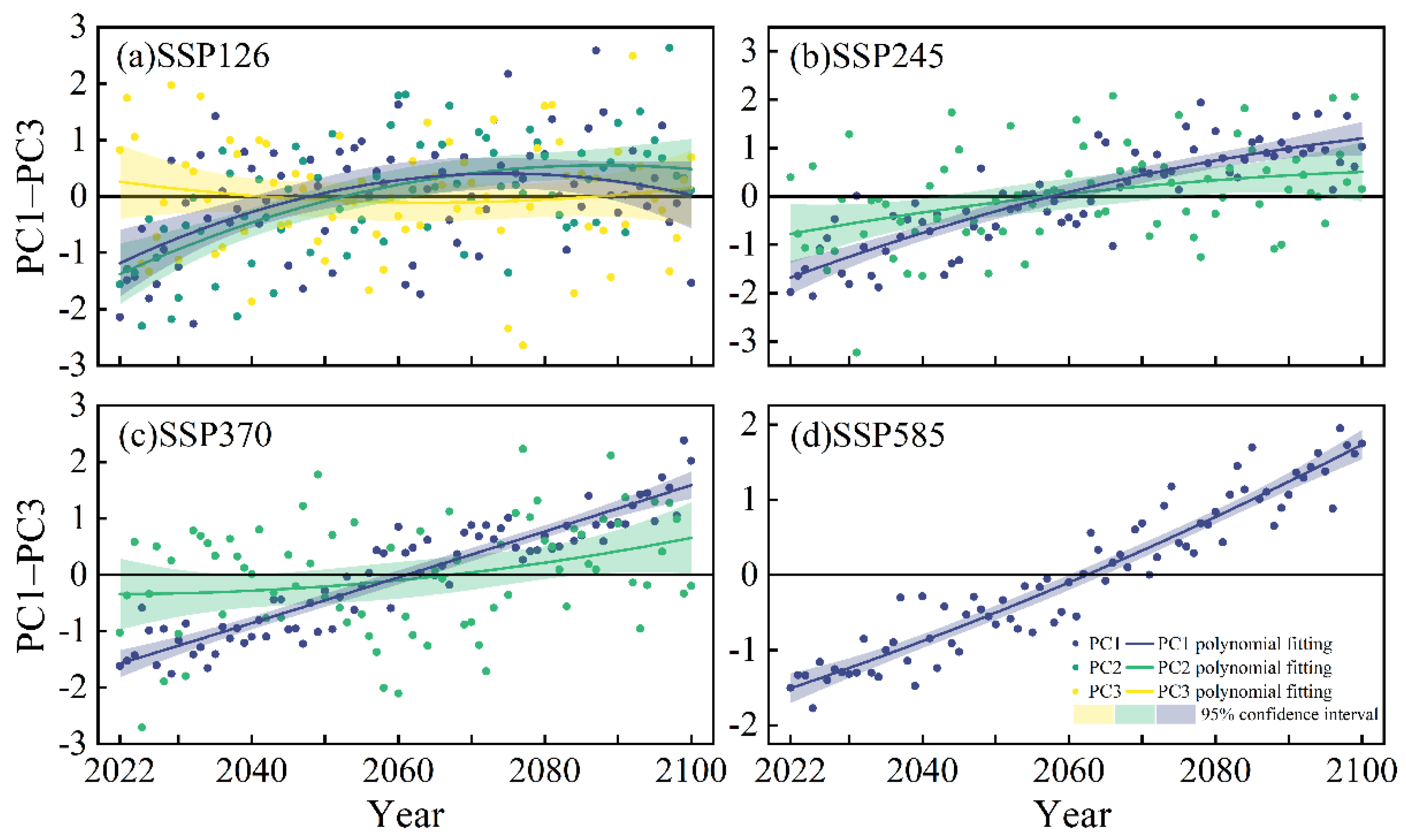
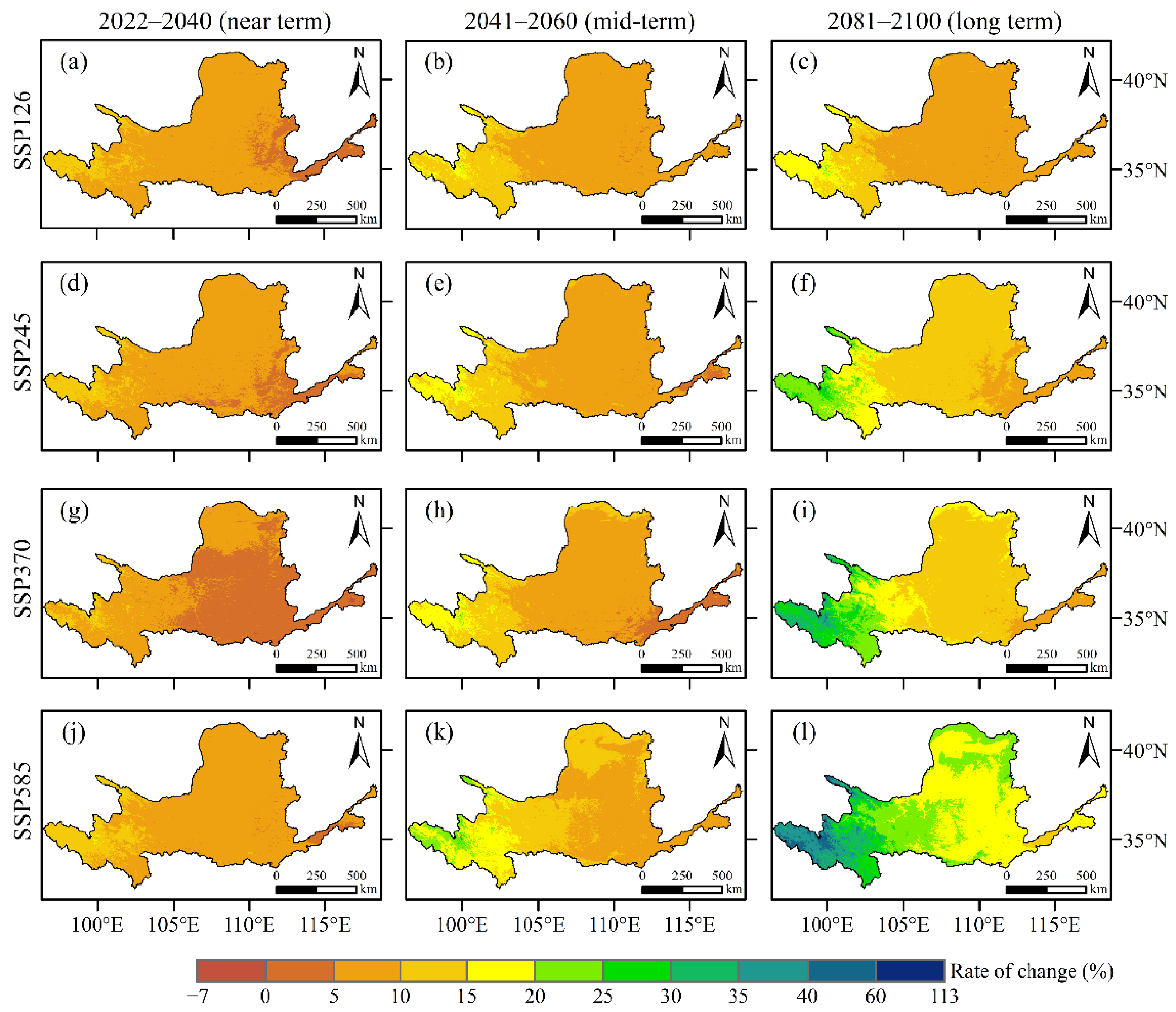
3.4. Spatial Evolution Characteristics of ET0

The EOF analysis of ET0 was conducted under four future emission scenarios in the YRB for 2022–2100, and the results were tested for modal significance using the North test, which are presented in Table 2 and Figure 10 and Figure 11. As presented in Table 2, the first three modes of ET0 in SSP126 passed the North test with a cumulative variance contribution of 88.68%; the first two modes of ET0 in SSP245 passed the North test with a cumulative variance contribution of 90.18%; the first two modes of ET0 in SSP370 passed the North test with a cumulative variance contribution of 94.32%; and the first mode of ET0 in SSP585 passed the North test with a cumulative variance contribution of 93.55%.
Under the SSP126 scenario, the first EOF modal eigenvector (EOF1) of ET0 in the YRB was positive, reflecting a spatially consistent trend of ET0 across the region, and exhibited an increasing trend from the northwest to the southeast, indicating a more pronounced increase in ET0 in the lower YRB (Figure 10a). EOF2 and EOF3, which explained 20.56% of the variations, reflected the secondary spatial characteristics of ET0 with opposite trends from northwest to southeast and from north to south (Figure 10b,c). Combined with the temporal coefficients (Figure 11a), PC1 and PC2 exhibited roughly the same trend, with an increasing trend from 2022 to 2100, particularly after the 2150s when PC1 and PC2 remained positive, indicating that ET0 remained high throughout this period. PC3 fluctuated at a value of approximately 0, reflecting no significant trend in ET0. Under SSP245 and SSP370, the EOF1 eigenvectors of ET0 in the basin were all positive, exhibiting spatial trends of larger values in the upper and middle reaches and smaller values in the lower reaches, as well as larger values in the central and western parts and smaller values in the northern and eastern parts (Figure 10d,f). All the EOF2 eigenvectors exhibited a secondary spatial trend of positive in the northwest and negative in the rest of the basin, with a relatively larger increase in ET0 near the source area in the upper part of the basin and a relatively larger decrease in ET0 in the south. Combined with the temporal coefficients (Figure 11b,c), PC1 and PC2 exhibited an increasing trend from 2022 to 2100 under the SSP245 and SSP370 scenarios, and PC1 increased more than PC2, particularly after the 2060s, when PC1 and PC2 always maintained positive values, indicating that ET0 remained high during this period. The distribution of EOF1 eigenvectors for ET0 in the basin under the SSP585 scenario was similar to that of EOF1 under the SSP245 scenario (Figure 10h), with an increasing trend in the time coefficient PC1 (Figure 11d), indicating an increasing trend in ET0 in the basin and a significant increase in ET0 after the 2060s.
As observed from the spatial variations in annual ET0 in the YRB in the near-, mid-, and long-term future relative to historical periods in the 21st century (Figure 12), the near-annual ET0 growth was generally low on an annual scale, and the rate of ET0 change was even negative in parts of Tai’an, Shandong Province, located in the lower reaches of the YRB, at −6.09% under the SSP370 scenario. In the mid- and long-term future scenarios, the ET0 rate of change gradually increased in the whole basin, and the areas with high ET0 variations were primarily concentrated in the YRB source area and a small part of the northern basin. In the lower reaches, the ET0 change rate was low, and the variations were spatially distributed as high in the west and low in the east. As the radiative forcing increased, the increase in ET0 became more significant, ranging from −3.08 to 50.78% under SSP126, from −1.32 to 68.88% under SSP245, from −6.09 to 89.30% under SSP370, and from −1.27 to 112.91% under SSP585. A maximum variation of 112.91% was observed in the western part of the YRB in the long-term future (2081–2100) under the SSP585 scenario.

4. Discussion

4.1. Influence of the ET0 Model

The models commonly used internationally for ET0 estimation can generally be divided into four major categories [54]: temperature methods, such as the Hargreaves [50] and Blaney–Criddle models [55]; mass transfer methods, such as the Rohwer [56] and Penman models [57]; radiation methods, such as the Priestley–Taylor [58] and Jensen–Haise models [59]; and synthesis methods, such as the Penman–Monteith model [4]. Although the Penman–Monteith model is considered the standard method for calculating ET0, accurate predictions of future ET0 in watersheds require more reliable meteorological data, and the outputs of existing GCMs and downscaling methods typically have low modeling accuracy for meteorological parameters such as wind speed, relative humidity, and radiation. Compared to other models, temperature-based models have lower data requirements and are computationally simple, and downscaling methods have a clear advantage in modeling temperature [60,61], with correlation coefficients generally above 0.90 (Figure 6), making them more widely applicable [31]. In addition, several studies have revealed strong relationships between future ET0 and temperature in other basins or regions. Xing et al. [27] attributed the increase in ET0 in the 21st century to an increase in temperature, and Ding and Peng [31] found that global warming led to a change in the main sensitive factor for potential evapotranspiration in the Loess Plateau from the average temperature in the historical period to the maximum temperature in the future period. The results of both these studies theoretically supported the use of the temperature-based ET0 model. Ahmadi and Baaghideh [25] explored the effect of climate change on ET0 in pistachio cultivation areas in Iran using the Hargreaves model. Yan and Mohammadian [47] evaluated the performance of the evaporation model based on the Hargreaves formulation using various fitting methods, and the results showed that the simulation was satisfactory. Among the many ET0 simplification methods, this study also selected the Hargreaves model, a temperature method recommended by the FAO [4] and researchers [62,63], to estimate the spatial and temporal characteristics of ET0 in the YRB under four future emission scenarios. The fitted scatter density plot had an R2 of 0.8523 at the monthly scale (Figure 7). The Hargreaves model can effectively simulate basin ET0; reflecting the rationality of the formula selection in this study. Notably, this study only considered the effect of temperature on ET0, thus, there may be some bias in the estimation results. The applicability of temperature models in specific regions [64,65] should be improved, and the effect of other meteorological elements on future ET0 [66] should be explored in future studies.

4.2. Spatial and Temporal Variations in Future ET0

As a result of global climate change, the hydrometeorological elements and hydrological environment of the YRB have been significantly affected [67]. Although many studies have examined the trends and attribution of ET0 in the YRB [36,68], previous studies were based on site-scale and historical data. Studies on future water balance and hydrological cycles in the YRB are relatively weak owing to the lack of studies on ET0.
This study predicted ET0 trends in the YRB for different periods under four future emission scenarios based on CMIP6 temperature data with high spatial and temporal resolution generated by the delta statistical downscaling method and the Hargreaves model. This study revealed an overall significant increase in ET0 in the YRB from 2022 to 2100 (p < 0.01) (Figure 8), without the “evaporation paradox” [69], which is similar to the future ET0 trends predicted by many studies [28,69,70]. Based on the Hargreaves model (i.e., Equation (2)), the change in ET0 is proportional to tas and the difference between tasmax and tasmin. With general global warming, tas, tasmax, and tasmin in the YRB in the future period showed sudden increases relative to the historical period (Figure S1). Therefore, the abrupt increase of ET0 can be attributed to the abrupt increase of temperature-like variables in the future period [27]. Radiative forcing is expected to stabilize at 2.6 W/m2 by 2100 for SSP126 and 8.5 W/m2 by 2100 for SSP585, and radiation values and temperature are positively related to ET0 [4]. The positive effects of increasing climatic factors, such as temperature and radiation, on ET0 in the YRB were greater than the negative effects of other factors, and therefore, the latter trend was greater than the former as emission concentrations increased in the YRB (Figure 8). The ET0 changes in the YRB in the near-, mid-, and long-term future under different future scenarios exhibited high spatial heterogeneity (Figure 10 and Figure 12), with a spatial distribution high in the west and low in the east, and the ET0 increase became more significant as the radiative forcing scenario increased. Consistent with the results of Ding and Peng [31], the increase in ET0 was generally greater at higher elevations than at lower elevations in the basin, with the most pronounced change in ET0 in the western part of the basin, reaching a maximum variation of 112.91% compared to that in the historical period (Figure 12). According to the ET0 equation (i.e., Equation (2)) and Figure S2, this change can be attributed to the largest temperature difference between tasmax and tasmin in the western part of the basin. In addition, as shown in the change in future precipitation in the YRB relative to the historical period (Figure S3), precipitation in the western part of the basin showed less growth overall and even negative growth in some phases. Warming and decreasing precipitation caused an increase in dryness in the western part of the basin, and the warm-dry trend intensified. Wang et al. [71] found that the evapotranspiration process was more sensitive to relative humidity in the western part of the basin, and a decrease in relative humidity caused an increase in evapotranspiration. Therefore, ET0 predictions based on the Hargreaves model were greater in these areas. Water loss in the YRB is likely to accelerate in the future than in historical periods, which will threaten the food and ecological security of the region; thus, developing flexible mitigation strategies tailored to local conditions is critical to coping with climate change [72].

4.3. Climate Model Uncertainty Analysis

Because of the differences in the feedback processes of different GCMs, a certain degree of uncertainty exists in their response to future greenhouse gas emissions, and the actual generalized optimal climate models and ET0 models cannot be determined [73]. Inevitable uncertainties exist in future ET0 predictions stemming from climate scenarios, climate models, and ET0 models [74], which greatly affect the confidence of the prediction results.
In response to the uncertainty of climate scenarios, this study selected the CMIP6 data, which had the largest number of participating models, the richest design of numerical experiments, and the largest amount of simulated data available than other CMIP generations for more than 20 years of the CMIP [37,75], initiated by the current Working Group on Coupled Models (WGCM). Compared to previous generations (CMIP3, CMIP5, etc.), CMIP6 uses a new scenario combining shared socio-economic pathways and typical concentration pathways to constrain multi-model predictions of key climate change indicators such as global surface temperature and ocean heat content based on historical observations, climate simulations, and climate sensitivity awareness, reducing uncertainty in predictions and providing higher resolution and reliability [76], thereby making the results more informative and time-sensitive than those based on CMIP5 for future ET0 studies, such as in Ahmadi and Baaghideh [25], Ding and Peng [31], Kundu et al. [6] and Le and Bae [77]. In response to the uncertainty of climate models, this study selected 24 GCMs with historical and future emission scenarios, which is more extensive than the studies of Li et al. [70], which only used one climate model (HadCM3) under two emission scenarios (A2 and B2), and Nooni et al. [1], which used only one climate model (CNRM-CM6). In addition, this study reduced the uncertainty of future temperature data by preferentially selecting climate models based on multiple interpolation methods, multiple evaluation indicators, and equal weight sets on a downscaling basis. The MAE was controlled within 2.5 mm, S and SS were approximately 1, and TS was approximately 0, indicating very high simulation accuracy (Table 3). Wang and Chen [24] reduced the spatial resolution of GCMs’ data to 0.5° based on the delta method, and the MAE of tas was in the range of 1.6–5.7 °C. However, the MAE of tas in this study was controlled in the range of 2.2–2.6 °C and had a higher spatial resolution of 1 km.
Although this study provides a comprehensive theoretical basis for future ET0 assessments, the uncertainties in the downscaling of GCMs [78] and in the selection and accuracy of ET0 models [74] may impact the prediction results. To improve ET0 estimates in future studies, consideration should be given to the long-term goal of the United Nations Framework Convention on Climate Change (Paris Agreement) to limit the increase in global average temperature to less than 2 °C compared to the pre-industrial period and to further efforts to limit it to less than 1.5 °C [79], as well as to achieve China’s 2060 carbon neutrality and global carbon neutrality. Describing and quantifying the relative importance of various uncertainty sources and the risks they pose in the assessment is important in current and future climate change impact studies and water resource assessments that should be strengthened to reduce prediction uncertainty.

5. Conclusions

Based on the 24 GCMs in CMIP6 and temperature data with high spatial and temporal resolution generated by the delta statistical downscaling model, this study assessed the evolution of ET0 in the YRB under four emission scenarios (SSP126, SSP245, SSP370, and SSP585) for the near (2022–2040), mid- (2041–2060), and long (2081–2100) term future. The major conclusions are as follows:
The regionally high-precision climate data generated by delta statistical downscaling based on multiple interpolation methods reduced the uncertainty in the GCM dataset. For the YRB, tas selected the climate models ACCESS-ESM1-5, CMCC-CM2-SR5, and INM-CM5-0; tasmax selected ACCESS-CM2, ACCESS-ESM1-5, and MRI-ESM2-0; and tasmin selected ACCESS-CM2, ACCESS-ESM1-5, and MPI-ESM1-2-LR. The equal-weighted multi-model ensemble had smaller mean absolute errors and higher correlation coefficients than single climate models, and CMIP6 efficiently simulated the temperature and ET0 in the YRB.
Compared with that of the historical period (1901–2014), the annual ET0 in the YRB under different emission scenarios (SSP126, SSP245, SSP370, and SSP585) in the future (2022–2100) substantially increased; the rate increased with the increase in emission concentration, and the ET0 in 2100 under the SSP585 scenario reached 1170.39 mm. Morlet wavelet analysis revealed that ET0 in the YRB had cyclic patterns of 34–38, 34, 39, and 27–32 years under the SSP126, SSP245, SSP370, and SSP585 scenarios, respectively.
Compared with that in the historical period, the ET0 variation in the YRB in the near-, mid-, and long-term future under different future scenarios exhibited strong spatial heterogeneity. EOF analysis revealed that ET0 had positive EOF1 values under all four emission scenarios, exhibiting a spatially consistent trend of ET0 variation across the region. A maximum variation of 112.91% occurred in the western part of the YRB in the long-term future (2081–2100) under the SSP585 scenario. Without a scientific response, future increases in ET0 could further reduce the shortage of water resources in the YRB.

Supplementary Materials

The following supporting information can be downloaded at: https://www.mdpi.com/article/10.3390/rs14225674/s1. Figure S1: Interannual variations in tas (a)/tasmax (b)/tasmin (c) in the Yellow River Basin over the historical period (1901–2014) and under different future emission scenarios; Figure S2: Spatial variations in the near (2022–2040; (a,d,g,j)), mid- (2041–2060; (b,e,h,k)), and long (2081–2100; (c,f,i,l)) term future difference between tasmax and tasmin of the Yellow River Basin relative to the historical period (1901–2014) under four SSP scenarios (SSP126, SSP245, SSP370, and SSP585); Figure S3: Spatial variations in the near (2022–2040; (a,d,g,j)), mid- (2041–2060; b,e,h,k), and long (2081–2100; (c,f,i,l)) term future annual precipitation of the Yellow River Basin relative to the historical period (1901–2014) under four SSP scenarios (SSP126, SSP245, SSP370, and SSP585).

Author Contributions

Conceptualization, S.J. and A.W.; methodology, C.S.; validation, S.J., A.W. and C.S.; investigation, A.W.; resources, S.J.; data curation, A.W.; writing—original draft, S.J. and A.W.; writing—review and editing, C.S. and K.W.; supervision, A.W. and K.W.; funding acquisition, S.J. and C.S. All authors have read and agreed to the published version of the manuscript.

Funding

This research was funded by the Training Program for Young Backbone Teachers in Colleges and Universities of Henan Province (2021GGJS003), the Henan Natural Science Foundation (212300410413), the Henan Youth Talent Promotion Project (2021HYTP030), the China Postdoctoral Science Foundation (2020M672247), the Key Science and Technology Project of Henan Province (No. 222102320108), and the First-class Project Special Funding of Yellow River Laboratory (No. YRL22IR12).

Institutional Review Board Statement

Not applicable.

Informed Consent Statement

Not applicable.

Data Availability Statement

Not applicable.

Conflicts of Interest

The authors declare no conflict of interest.

References

  1. Nooni, I.K.; Hagan, D.F.T.; Wang, G.; Ullah, W.; Lu, J.; Li, S.; Dzakpasu, M.; Prempeh, N.A.; Lim Kam Sian, K.T.C. Future Changes in Simulated Evapotranspiration across Continental Africa Based on CMIP6 CNRM-CM6. Int. J. Environ. Res. Public Health. 2021, 18, 6760. [Google Scholar] [CrossRef] [PubMed]
  2. Wang, T.; Tu, X.; Singh, V.P.; Chen, X.; Lin, K. Global data assessment and analysis of drought characteristics based on CMIP6. J. Hydrol. 2021, 596, 126091. [Google Scholar] [CrossRef]
  3. Zhang, Y.; Fu, B.; Feng, X.; Pan, N. Response of Ecohydrological Variables to Meteorological Drought under Climate Change. Remote Sens. 2022, 14, 1920. [Google Scholar] [CrossRef]
  4. Allen, R.G.; Pereira, L.S.; Raes, D.; Smith, M. Crop Evapotranspiration-Guidelines for Computing Crop Water Requirements; FAO Irrigation and Drainage Paper 56; FAO: Rome, Italy, 1998. [Google Scholar]
  5. Liu, Y.; Yue, Q.; Wang, Q.; Yu, J.; Zheng, Y.; Yao, X.; Xu, S. A Framework for Actual Evapotranspiration Assessment and Projection Based on Meteorological, Vegetation and Hydrological Remote Sensing Products. Remote Sens. 2021, 13, 3643. [Google Scholar] [CrossRef]
  6. Kundu, S.; Mondal, A.; Khare, D.; Hain, C.; Lakshmi, V. Projecting Climate and Land Use Change Impacts on Actual Evap-otranspiration for the Narmada River Basin in Central India in the Future. Remote Sens. 2018, 10, 578. [Google Scholar] [CrossRef] [Green Version]
  7. Shi, L.; Feng, P.; Wang, B.; Liu, D.L.; Zhang, H.; Liu, J.; Yu, Q. Assessing future runoff changes with different potential evapotranspiration inputs based on multi-model ensemble of CMIP5 projections. J. Hydrol. 2022, 612, 128042. [Google Scholar] [CrossRef]
  8. Zeng, P.; Sun, F.; Liu, Y.; Feng, H.; Zhang, R.; Che, Y. Changes of potential evapotranspiration and its sensitivity across China under future climate scenarios. Atmos. Res. 2021, 261, 105763. [Google Scholar] [CrossRef]
  9. Guo, D.; Westra, S.; Maier, H.R. Sensitivity of potential evapotranspiration to changes in climate variables for different Aus-tralian climatic zones. Hydrol. Earth Syst. Sci. 2017, 21, 2107–2126. [Google Scholar] [CrossRef] [Green Version]
  10. Jhajharia, D.; Dinpashoh, Y.; Kahya, E.; Singh, V.P.; Fakheri-Fard, A. Trends in reference evapotranspiration in the humid region of northeast India. Hydrol. Process. 2012, 26, 421–435. [Google Scholar] [CrossRef]
  11. Kuang, X.; Jiao, J.J. Review on climate change on the Tibetan Plateau during the last half century. J. Geophys. Res. Atmos. 2016, 121, 3979–4007. [Google Scholar] [CrossRef]
  12. PascoliniCampbell, M.; Reager, J.T.; Chandanpurkar, H.A.; Rodell, M. Retraction Note: A 10 per cent increase in global land evapotranspiration from 2003 to 2019. Nature 2022, 604, 202. [Google Scholar] [CrossRef] [PubMed]
  13. She, D.; Xia, J.; Zhang, Y. Changes in reference evapotranspiration and its driving factors in the middle reaches of Yellow River Basin, China. Sci. Total Environ. 2017, 607–608, 1151–1162. [Google Scholar] [CrossRef] [PubMed]
  14. Yagob, D.; Deepak, J.; Ahmad, F.; Vijay, P.S.; Ercan, K. Trends in reference crop evapotranspiration over Iran. J. Hydrol. 2011, 399, 422–433. [Google Scholar]
  15. Huang, J.; Zhai, J.; Jiang, T.; Wang, Y.; Li, X.; Wang, R.; Xiong, M.; Su, B.; Fischer, T. Analysis of future drought characteristics in China using the regional climate model CCLM. Clim. Dyn. 2018, 50, 507–525. [Google Scholar] [CrossRef]
  16. Torres, R.R.; Marengo, J.A. Climate change hotspots over South America: From CMIP3 to CMIP5 multi-model datasets. Theor. Appl. Climatol. 2014, 117, 579–587. [Google Scholar] [CrossRef]
  17. Chen, H.; Guo, J.; Xiong, W.; Guo, S.; Xu, C. Downscaling GCMs using the Smooth Support Vector Machine method to predict daily precipitation in the Hanjiang Basin. Adv. Atmos. Sci. 2010, 27, 274–284. [Google Scholar] [CrossRef]
  18. Harding, K.J.; Snyder, P.K. Examining future changes in the character of Central U.S. warm-season precipitation using dynamical downscaling. J. Geophys. Res.-Atmos. 2014, 119, 13116–13136. [Google Scholar] [CrossRef] [Green Version]
  19. Giorgi, F.; Mearns, L.O. Approaches to the simulation of regional climate change: A review. Rev. Geophys. 1991, 29, 191–216. [Google Scholar] [CrossRef]
  20. Benestad, R.E. A comparison between two empirical downscaling strategies. Int. J. Climatol. 2001, 21, 1645–1668. [Google Scholar] [CrossRef]
  21. Peng, S.; Ding, Y.; Wen, Z.; Chen, Y.; Cao, Y.; Ren, J. Spatiotemporal change and trend analysis of potential evapotranspiration over the Loess Plateau of China during 2011–2100. Agric. For. Meteorol. 2017, 233, 183–194. [Google Scholar] [CrossRef] [Green Version]
  22. Xu, J.; Gao, Y.; Chen, D.; Xiao, L.; Ou, T. Evaluation of global climate models for downscaling applications centred over the Tibetan Plateau. Int. J. Climatol. 2017, 37, 657–671. [Google Scholar] [CrossRef]
  23. Dosio, A.; Panitz, H.; Schubert-Frisius, M.; Lüthi, D. Dynamical downscaling of CMIP5 global circulation models over CORDEX-Africa with COSMO-CLM: Evaluation over the present climate and analysis of the added value. Clim. Dyn. 2015, 44, 2637–2661. [Google Scholar] [CrossRef] [Green Version]
  24. Wang, L.; Chen, W. A CMIP5 multimodel projection of future temperature, precipitation, and climatological drought in China. Int. J. Climatol. 2014, 34, 2059–2078. [Google Scholar] [CrossRef]
  25. Ahmadi, H.; Baaghideh, M. Assessment of anomalies and effects of climate change on reference evapotranspiration and water requirement in pistachio cultivation areas in Iran. Arab. J. Geosci. 2020, 13, 332. [Google Scholar] [CrossRef]
  26. Das, S.; Datta, P.; Sharma, D.; Goswami, K. Trends in Temperature, Precipitation, Potential Evapotranspiration, and Water Availability across the Teesta River Basin under 1.5 and 2 °C Temperature Rise Scenarios of CMIP6. Atmosphere. 2022, 13, 941. [Google Scholar] [CrossRef]
  27. Xing, W.; Wang, W.; Shao, Q.; Peng, S.; Yu, Z.; Yong, B.; Taylor, J. Changes of reference evapotranspiration in the Haihe River Basin: Present observations and future projection from climatic variables through multi-model ensemble. Glob. Planet. Change 2014, 115, 1–15. [Google Scholar] [CrossRef]
  28. Liu, X.; Li, C.; Zhao, T.; Han, L. Future changes of global potential evapotranspiration simulated from CMIP5 to CMIP6 models. Atmos. Ocean. Sci. Lett. 2020, 13, 568–575. [Google Scholar] [CrossRef]
  29. Nistor, M.; Mîndrescu, M.; Petrea, D.; Nicula, A.; Rai, P.K.; Benzaghta, M.A.; Dezsi, Ş.; Hognogi, G.; Porumb-Ghiurco, C.G. Climate change impact on crop evapotranspiration in Turkey during the 21st Century. Meteorol. Appl. 2019, 26, 442–453. [Google Scholar] [CrossRef] [Green Version]
  30. Zhang, Q.; Zhang, Z.; Shi, P.; Singh, V.P.; Gu, X. Evaluation of ecological instream flow considering hydrological alterations in the Yellow River basin, China. Glob. Planet. Change 2018, 160, 61–74. [Google Scholar] [CrossRef]
  31. Ding, Y.; Peng, S. Spatiotemporal change and attribution of potential evapotranspiration over China from 1901 to 2100. Theor. Appl. Climatol. 2021, 145, 79–94. [Google Scholar] [CrossRef]
  32. Pan, S.; Xu, Y.; Xuan, W.; Gu, H.; Bai, Z. Appropriateness of Potential Evapotranspiration Models for Climate Change Impact Analysis in Yarlung Zangbo River Basin, China. Atmosphere 2019, 10, 453. [Google Scholar] [CrossRef]
  33. Zhu, Y.; Chang, J.; Huang, S.; Huang, Q. Characteristics of integrated droughts based on a nonparametric standardized drought index in the Yellow River Basin, China. Hydrol. Res. 2016, 47, 454–467. [Google Scholar] [CrossRef]
  34. Sheng, X.Y.; Wang, J.K.; Cui, Q.T.; Zhang, W.; Zhu, X.F. A feasible biochar derived from biogas residue and its application in the efficient adsorption of tetracycline from an aqueous solution. Environ. Res. 2022, 207, 112175. [Google Scholar] [CrossRef] [PubMed]
  35. Yin, L.; Feng, X.; Fu, B.; Wang, S.; Wang, X.; Chen, Y.; Tao, F.; Hu, J. A coupled human-natural system analysis of water yield in the Yellow River basin, China. Sci. Total Environ. 2021, 762, 143141. [Google Scholar] [CrossRef] [PubMed]
  36. Zhao, F.; Ma, S.; Wu, Y.; Qiu, L.; Wang, W.; Lian, Y.; Chen, J.; Sivakumar, B. The role of climate change and vegetation greening on evapotranspiration variation in the Yellow River Basin, China. Agric. For. Meteorol. 2022, 316, 108842. [Google Scholar] [CrossRef]
  37. O’Neill, B.C.; Tebaldi, C.; van Vuuren, D.P.; Eyring, V.; Friedlingstein, P.; Hurtt, G.; Knutti, R.; Kriegler, E.; Lamarque, J.; Lowe, J.; et al. The Scenario Model Intercomparison Project (ScenarioMIP) for CMIP6. Geosci. Model Dev. 2016, 9, 3461–3482. [Google Scholar] [CrossRef] [Green Version]
  38. Zhang, Z.H.; Deng, S.F.; Zhao, Q.D.; Zhang, S.Q.; Zhang, X.W. Projected glacier meltwater and river run-off changes in the Upper Reach of the Shule River Basin, north-eastern edge of the Tibetan Plateau. Hydrol. Process. 2019, 33, 1059–1074. [Google Scholar] [CrossRef]
  39. Hay, L.E.; Wilby, R.; Leavesley, G.H. A comparison of delta change and downscaled GCM scenarios for three mountainous basins in the United States. J. Am. Water Resour. Assoc. 2000, 36, 387–397. [Google Scholar] [CrossRef]
  40. Willmott, C.J.; Matsuura, K. Advantages of the mean absolute error (MAE) over the root mean square error (RMSE) in assessing average model performance. Clim. Res. 2005, 30, 79–82. [Google Scholar] [CrossRef]
  41. Taylor, K.E. Summarizing multiple aspects of model performance in a single diagram. J. Geophys. Res. Atmos. 2001, 106, 7183–7192. [Google Scholar] [CrossRef]
  42. Jiang, Z.; Song, J.; Li, L.; Chen, W.; Wang, Z.; Wang, J. Extreme climate events in China: IPCC-AR4 model evaluation and projection. Clim. Change 2012, 110, 385–401. [Google Scholar] [CrossRef]
  43. Chen, W.; Jiang, Z.; Li, L. Probabilistic Projections of Climate Change over China under the SRES A1B Scenario Using 28 AOGCMs. J. Clim. 2011, 24, 4741–4756. [Google Scholar] [CrossRef] [Green Version]
  44. Jiang, D.; Wang, H.; Lang, X. Evaluation of East Asian Climatology as Simulated by Seven Coupled Models. Adv. Atmos. Sci. 2005, 22, 479–495. [Google Scholar]
  45. Ma, Z.; Sun, P.; Zhang, Q.; Zou, Y.; Lv, Y.; Li, H.; Chen, D. The Characteristics and Evaluation of Future Droughts across China through the CMIP6 Multi-Model Ensemble. Remote Sens. 2022, 14, 1097. [Google Scholar] [CrossRef]
  46. Pelosi, A.; Medina, H.; Villani, P.; Urso, D.G.; Chirico, G.B. Probabilistic forecasting of reference evapotranspiration with a limited area ensemble prediction system. Agric. Water Manag. 2016, 178, 106–118. [Google Scholar] [CrossRef]
  47. Yan, X.; Mohammadian, A. Estimating future daily pan evaporation for Qatar using the Hargreaves model and statistically downscaled global climate model projections under RCP climate change scenarios. Arab. J. Geosci. 2020, 13, 938. [Google Scholar] [CrossRef]
  48. Hargreaves, G.H. Moisture Availability and Crop Production. Trans. ASAE 1975, 18, 980–0984. [Google Scholar] [CrossRef]
  49. Hargreaves, G.H.; Samani, Z.A. Estimating Potential Evapotranspiration. J. Irrig. Drain. Div. 1982, 108, 225–230. [Google Scholar] [CrossRef]
  50. Hargreaves, G.H.; Samani, Z.A. Reference Crop Evapotranspiration from Temperature. Appl. Eng. Agric. 1985, 2, 96–99. [Google Scholar] [CrossRef]
  51. Li, H.; Wang, Y.; Jia, L.; Wu, Y.; Xie, M. Runoff Characteristics of the Nen River Basin and its Cause. J. Mt. Sci. 2014, 11, 110–118. [Google Scholar] [CrossRef]
  52. Naren, A.; Maity, R. Modeling of local sea level rise and its future projection under climate change using regional information through EOF analysis. Theor. Appl. Climatol. 2018, 134, 1269–1285. [Google Scholar] [CrossRef]
  53. North, G.R.; Bell, T.L.; Cahalan, R.F.; Moeng, F.J. Sampling Errors in the Estimation of Empirical Orthogonal Functions. Am. Meteorol. Soc. 1982, 110, 699–706. [Google Scholar] [CrossRef]
  54. Singh, V.P.; Xu, C.Y. Evaluation and generalization of 13 mass-transfer equations for determining free water evaporation. Hydrol. Process. 1997, 3, 311–323. [Google Scholar] [CrossRef]
  55. Blaney, H.F.; Criddle, W.D. Determining Consumptive Use and Irrigation Water Requirements. Tech. Bull. 1962, 4, 369–373. [Google Scholar]
  56. Rohwer, C. Evaporation from a Free Water Surface; US Department of Agriculture: Washington, DC, USA, 1931.
  57. Penman, H.L. Natural Evaporation from Open Water, Bare Soil and Grass. Proc. R. Soc. Lond. Ser. A Math. Phys. Sci. 1948, 193, 120–145. [Google Scholar]
  58. Priestley, C.H.B.; Taylor, R.J. On the Assessment of Surface Heat Flux and Evaporation Using Large-Scale Parameters. Mon. Weather Rev. 1972, 100, 81–92. [Google Scholar] [CrossRef]
  59. Jensen, M.E.; Haise, H.R. Estimating Evapotranspiration from Solar Radiation. J. Irrig. Drain. Div. 1963, 89, 15–41. [Google Scholar] [CrossRef]
  60. Peng, S.; Gang, C.; Cao, Y.; Chen, Y. Assessment of climate change trends over the Loess Plateau in China from 1901 to 2100. Int. J. Climatol. 2018, 38, 2250–2264. [Google Scholar] [CrossRef]
  61. Yang, X.; Zhou, B.; Xu, Y.; Han, Z. CMIP6 Evaluation and Projection of Temperature and Precipitation over China. Adv. Atmos. Sci. 2021, 38, 817–830. [Google Scholar] [CrossRef]
  62. Er-Raki, S.; Chehbouni, A.; Khabba, S.; Simonneaux, V.; Jarlan, L.; Ouldbba, A.; Rodriguez, J.C.; Allen, R. Assessment of reference evapotranspiration methods in semi-arid regions: Can weather forecast data be used as alternate of ground meteorological parameters? J. Arid. Environ. 2010, 74, 1587–1596. [Google Scholar] [CrossRef] [Green Version]
  63. Zhao, C.; Nan, Z.; Feng, Z. GIS-assisted spatially distributed modeling of the potential evapotranspiration in semi-arid climate of the Chinese Loess Plateau. J. Arid. Environ. 2004, 58, 387–403. [Google Scholar]
  64. Bourletsikas, A.; Argyrokastritis, I.; Proutsos, N. Comparative evaluation of 24 reference evapotranspiration equations applied on an evergreen-broadleaved forest. Hydrol. Res. 2018, 49, 1028–1041. [Google Scholar] [CrossRef]
  65. Lang, D.; Zheng, J.; Shi, J.; Liao, F.; Ma, X.; Wang, W.; Chen, X.; Zhang, M. A Comparative Study of Potential Evapotranspiration Estimation by Eight Methods with FAO Penman–Monteith Method in Southwestern China. Water 2017, 9, 734. [Google Scholar] [CrossRef] [Green Version]
  66. Yan, X.; Mohammadian, A. Forecasting daily reference evapotranspiration for Canada using the Penman-Monteith model and statistically downscaled global climate model projections. Alex. Eng. J. 2020, 59, 883–891. [Google Scholar] [CrossRef]
  67. Omer, A.; Elagib, N.A.; Ma, Z.; Saleem, F.; Mohammed, A. Water scarcity in the Yellow River Basin under future climate change and human activities. Sci. Total Environ. 2020, 749, 141446. [Google Scholar] [CrossRef]
  68. Jiang, Z.; Yang, Z.; Zhang, S.; Liao, C.; Hu, Z.; Cao, R.; Wu, H. Revealing the spatio-temporal variability of evapotranspiration and its components based on an improved Shuttleworth-Wallace model in the Yellow River Basin. J. Environ. Manag. 2020, 262, 110310. [Google Scholar] [CrossRef]
  69. Roderick, M.L.; Farquhar, G.D. The cause of decreased pan evaporation over the past 50 years. Science 2002, 298, 1410–1411. [Google Scholar] [CrossRef]
  70. Li, Z.; Zheng, F.; Liu, W. Spatiotemporal characteristics of reference evapotranspiration during 1961–2009 and its projected changes during 2011–2099 on the Loess Plateau of China. Agric. For. Meteorol. 2012, 154–155, 147–155. [Google Scholar] [CrossRef]
  71. Wang, W.; Shao, Q.; Peng, S.; Xing, W.; Yang, T.; Luo, Y.; Yong, B.; Xu, J. Reference evapotranspiration change and the causes across the Yellow River Basin during 1957-2008 and their spatial and seasonal differences. Water Resour. Res. 2012, 48, 113–122. [Google Scholar] [CrossRef]
  72. Cook, P.A.; Black, E.C.L.; Verhoef, A.; Macdonald, D.M.J.; Sorensen, J.P.R. Projected increases in potential groundwater recharge and reduced evapotranspiration under future climate conditions in West Africa. J. Hydrol. Reg. Stud. 2022, 41, 101076. [Google Scholar] [CrossRef]
  73. Gharbia, S.S.; Smullen, T.; Gill, L.; Johnston, P.; Pilla, F. Spatially distributed potential evapotranspiration modeling and climate projections. Sci. Total Environ. 2018, 633, 571–592. [Google Scholar] [CrossRef] [PubMed]
  74. Dallaire, G.; Poulin, A.; Arsenault, R.; Brissette, F. Uncertainty of potential evapotranspiration modelling in climate change impact studies on low flows in North America. Hydrol. Sci. J. 2021, 66, 689–702. [Google Scholar] [CrossRef]
  75. Liu, J.; Lu, Y. How Well Do CMIP6 Models Simulate the Greening of the Tibetan Plateau? Remote Sens. 2022, 14, 4633. [Google Scholar] [CrossRef]
  76. Stouffer, R.J.; Eyring, V.; Meehl, G.A.; Bony, S.; Senior, C.; Stevens, B.; Taylor, K.E. CMIP5 Scientific Gaps and Recommendations for CMIP6. Bull. Amer. Meteorol. Soc. 2017, 98, 95–105. [Google Scholar] [CrossRef]
  77. Le, T.; Bae, D. Response of global evaporation to major climate modes in historical and future Coupled Model Intercomparison Project Phase 5 simulations. Hydrol. Earth Syst. Sci. 2020, 24, 1131–1143. [Google Scholar] [CrossRef]
  78. Gao, C.; Booij, M.J.; Xu, Y. Assessment of extreme flows and uncertainty under climate change: Disentangling the uncertainty contribution of representative concentration pathways, global climate models and internal climate variability. Hydrol. Earth Syst. Sci. 2020, 24, 3251–3269. [Google Scholar] [CrossRef]
  79. Meinshausen, M.; Lewis, J.; McGlade, C.; Gütschow, J.; Nicholls, Z.; Burdon, R.; Cozzi, L.; Hackmann, B. Realization of Paris Agreement pledges may limit warming just below 2 °C. Nature 2022, 604, 304–309. [Google Scholar] [CrossRef]
Figure 1. (a) Location and digital elevation model of the Yellow River Basin in China and (b) the distribution of 93 national meteorological stations in the Yellow River Basin.
Remotesensing 14 05674 g001
Figure 2. The delta downscaling process of the climate models over the Yellow River Basin.
Remotesensing 14 05674 g002
Figure 3. Fitting performance ranking of 21 climate models simulating tas monthly series of the Yellow River Basin from 1995 to 2014 under different interpolation methods and evaluation metrics. a, b, c, d, and e under each evaluation method are the evaluation rankings of the five interpolation methods: BI, IDW, kriging, NNI, and spline, respectively. The higher the ranking, the higher the model’s fitting accuracy.
Remotesensing 14 05674 g003
Figure 4. Fitting performance ranking of 19 climate models simulating tasmax monthly series of the Yellow River Basin from 1995 to 2014 under different interpolation methods and evaluation metrics. a, b, c, d, and e under each evaluation method are the evaluation rankings of the five interpolation methods: BI, IDW, kriging, NNI, and spline, respectively. The higher the ranking, the higher the model’s fitting accuracy.
Remotesensing 14 05674 g004
Figure 5. Fitting performance ranking of 21 climate models simulating the tasmin monthly series of the Yellow River Basin from 1995 to 2014 under different interpolation methods and evaluation metrics. a, b, c, d, and e under each evaluation method are the evaluation rankings of the five interpolation methods: BI, IDW, kriging, NNI, and spline, respectively. The higher the ranking, the higher the model’s fitting accuracy.
Remotesensing 14 05674 g005
Figure 6. Scatter density plots of measured and selected climate models and multi-model ensembles simulating monthly temperatures in the Yellow River Basin at stations from 1995 to 2014. (ac) correspond to the fitting effects of ACCESS-ESM1-5, CMCC-CM2-SR5, and GISS-E2-1-G, respectively, under tas variable; (d) corresponds to the fitting effect of MMEtas; (eg) correspond to the fitting effects of ACCESS-CM2, ACCESS-ESM1-5, and MRI-ESM2-0, respectively, under tasmax variable; (h) corresponds to the fitting effect of MMEtasmax; (ik) correspond to the fitting effects of ACCESS-CM2, ACCESS-ESM1-5, and MPI-ESM1-2-LR, respectively, under tasmin variable; and (l) corresponds to the fitting effect of MMEtasmin.
Remotesensing 14 05674 g006
Figure 7. Scatter density plot of monthly observed pan evaporation converted values (ET0(pan)) and multi-model ensemble simulations (ET0(Har)) in the Yellow River Basin from 1980 to 2014.
Remotesensing 14 05674 g007
Figure 8. Interannual variations in ET0 in the Yellow River Basin over the historical period (1901–2014) and under different future emission scenarios (2022–2100; SSP126, SSP245, SSP370, and SSP585) (p is an indicator of significance obtained by the F-test).
Remotesensing 14 05674 g008
Figure 9. Wavelet analysis of ET0 in the Yellow River Basin under four future emission scenarios (SSP126, SSP245, SSP370, and SSP585), including wavelet coefficient contour plots of the real part (a,c,e,g) and wavelet variance plots (b,d,f,h).
Remotesensing 14 05674 g009
Figure 10. Main modal eigenvectors of the EOF of the ET0 spatial field in the Yellow River Basin for 2022–2100 under scenarios SSP126 (ac), SSP245 (d,e), SSP370 (f,g), and SSP585 (h), where SSP126/245/370/585–EOFi (contribution/%) in each figure represents the i-th modal eigenvector (EOFi) of ET0 under scenarios SSP126/245/370/585, with the contribution of each mode in parentheses. The red dashed lines in (b,c,e,g) are the positive and negative dividing lines of the eigenvectors.
Remotesensing 14 05674 g010
Figure 11. Principal component time coefficients (PC1–PC3) and their polynomial fits for the EOF analysis of future ET0 in the Yellow River Basin under four emission scenarios ((a) SSP126, (b) SSP245, (c) SSP370, and (d) SSP585).
Remotesensing 14 05674 g011
Figure 12. Spatial variations in the near (2022–2040; a,d,g,j), mid- (2041–2060; b,e,h,k), and long (2081–2100; c,f,i,l) term future annual ET0 of the Yellow River Basin relative to the historical period (1901–2014) under four SSP scenarios (SSP126, SSP245, SSP370, and SSP585).
Remotesensing 14 05674 g012
Table 1. Introduction to climate models with temperature variables.
Serial NumberClimate ModelsVariablesResearch Institution, CountrySpatial Resolution
1ACCESS-CM2tasmax, tasminACCESS, Australia1.9° × 1.3°
2ACCESS-ESM1-5tas, tasmax, tasminACCESS, Australia1.9° × 1.3°
3AWI-CM-1-1-MRtas, tasminAWI, Germany0.9° × 0.9°
4AWI-ESM-1-1-LRtasmax, tasminAWI, Germany1.9° × 1.9°
5BCC-CSM2-MRtas, tasmax, tasminBBC, CMA, China1.125° × 1.125°
6BCC-ESM1tasmax, tasminBBC, CMA, China2.8° × 2.8°
7CanESM5tas, tasmax, tasminCCCMA, Canada2.8125° × 2.8125°
8CMCC-CM2-SR5tasCMCC, Italy1.250° × 0.938°
9CMCC-ESM2tas, tasminCMCC, Italy1.25° × 0.9375°
10E3SM-1-0tasLLNL, ANL, LANL, LBNL, ORNL, PNNL, SNL, U.S.A1° × 1°
11EC-Earth3tas, tasmax, tasminEC-Earth, 10 European countries0.7° × 0.7°
12EC-Earth3-Vegtas, tasmax, tasminEC-Earth, 10 European countries0.703° × 0.703°
13FGOALS-f3-LtasIAP, CAS, China1° × 1.25°
14FIO-ESM-2-0tas, tasmax, tasminFIO, China0.9424° × 1.25°
15GFDL-ESM4tas, tasmax, tasminGFDL, U.S.A1° × 1.25°
16GISS-E2-1-Gtas, tasmax, tasminNASA-GISS, U.S.A1° × 1.25°
17INM-CM5-0tas, tasmax, tasminINM, Russia2° × 1.5°
18IPSL-CM6A-LRtas, tasmax, tasminIPSL, France1.2676° × 2.5°
19MIROC6tas, tasmax, tasminMIROC, Japan1.389° × 1.406°
20MPI-ESM-1-2-HAMtas, tasmax, tasminMPI, Germany1.865° × 1.875°
21MPI-ESM1-2-HRtas, tasmax, tasminMPI, Germany0.9375° × 0.9375°
22MPI-ESM1-2-LRtas, tasmax, tasminMPI, Germany1.875° × 1.875°
23MRI-ESM2-0tas, tasmax, tasminMRI, Japan1.124° × 1.125°
24NESM3tas, tasmax, tasminNUIST, China1.865° × 1.875°
Note: In the variable column, tas is the average temperature, tasmax is the average maximum temperature, and tasmin is the average minimum temperature.
Table 2. Main modes and contributions of ET0 under future climate scenarios in EOF analysis.
Climate ScenariosCorresponding ModesVariance ContributionCumulative Variance ContributionNorth Test
SSP126EOF168.12%68.12%pass
EOF213.51%81.63%pass
EOF37.05%88.68%pass
SSP245EOF181.75%81.75%pass
EOF28.43%90.18%pass
SSP370EOF189.85%89.85%pass
EOF24.47%94.32%pass
SSP585EOF193.55%93.55%pass
Table 3. Evaluation of the fitting error of downscaled climate models for monthly temperatures (tas/tasmax/tasmin) in the Yellow River Basin from January 1995 to December 2014.
ModelsTasTasmaxTasmin
MAESSSTSMAESSSTSMAESSSTS
ACCESS-CM2\\\\2.6754890.9998770.8898051.94 × 10−62.3389170.9975360.9159410.001035
ACCESS-ESM1-52.1964490.9847450.9266810.0017492.4974310.9742970.9014890.0004642.2950150.9636890.9171580.004465
AWI-CM-1-1-MR2.4428220.9995480.9092360.00021\\\\2.8378470.9656670.8810390.003347
AWI-ESM-1-1-LR\\\\2.7891430.9870860.8768860.002682.4708420.9900190.9076960.000134
BCC-CSM2-MR2.5482590.9861990.9046987.59 × 10−62.8860120.9794980.8716590.0002292.651750.9850430.894620.00095
BCC-ESM1\\\\2.8104140.9542780.8763250.001362.6172580.984850.8980640.005105
CanESM52.5537480.9657380.9008030.0024062.9097490.9806010.8670350.0078832.5724980.9708030.8980880.000166
CMCC-CM2-SR52.2737620.995010.9203462.77 × 10−6\\\\\\\\
CMCC-ESM22.3934240.9902470.9126770.001578\\\\2.4963310.993730.9050890.003913
E3SM-1-02.2648770.9909430.9212410.000168\\\\\\\\
EC-Earth32.3453910.9864130.915180.0012212.6306970.987090.8879310.0058392.451740.9808050.9058823.75 × 10−5
EC-Earth3-Veg2.5181350.9800410.9017820.0009442.7601980.98010.8775075.90 × 10−72.6539310.9764770.8872520.005208
FGOALS-f3-L2.3928950.9827420.9126699.79 × 10−8\\\\\\\\
FIO-ESM-2-02.390420.9860340.9131270.0006042.6604440.9893160.8885240.0033132.4835920.988290.9063823.56 × 10−6
GFDL-ESM42.4151560.9917490.9114210.0025982.7024980.9841360.8849430.0003812.4793620.992170.9024940.006418
GISS-E2-1-G2.29510.9926670.9193732.03 × 10−52.677670.9852820.8859170.0010972.3639760.9972950.9167920.000367
INM-CM5-02.3133180.9941960.9173275.45 × 10−52.6880340.9769840.8848530.0002012.4947030.9919610.9048550.000691
IPSL-CM6A-LR2.3664870.9861570.9151972.53 × 10−52.7092990.9595370.883370.0002682.4332050.9897670.9088170.001011
MIROC62.5389820.9752220.9033790.0024192.9447480.9774220.864460.0081822.5340290.9829930.9021850.000318
MPI-ESM-1-2-HAM2.4262830.9881530.9112447.45 × 10−52.7957970.977820.87740.0016992.4722260.9933530.9065090.000618
MPI-ESM1-2-HR2.4825150.9853070.909340.0001792.8130330.9848010.875780.0008552.4789920.9905030.9064712.68 × 10−5
MPI-ESM1-2-LR2.4401390.9908950.9125160.0006082.8255830.9871120.878010.0003332.444280.9948610.9095020.001426
MRI-ESM2-02.4304810.990840.9117750.0003862.7543170.9891830.8805035.16 × 10−72.4729970.9938230.9072910.001735
NESM32.3937440.9881310.9135260.001152.6254480.9899530.8901048.44 × 10−52.4751250.9921280.9075850.002775
Note: MAE, S, SS, and TS are mean absolute error, Taylor diagram-based quantifiers, spatial skill scores, and temporal skill scores, respectively. MAE is measured in °C, and the others are dimensionless indicators. The closer MAE and TS are to 0, the better the simulation ability of the model; the closer S and SS are to 1, the better the simulation ability of the model.
Publisher’s Note: MDPI stays neutral with regard to jurisdictional claims in published maps and institutional affiliations.

