Figure 1.
Reference data in study areas of Sherman, Thomas, Gray, and McPherson in Kansas, US.
Figure 1.
Reference data in study areas of Sherman, Thomas, Gray, and McPherson in Kansas, US.
Figure 2.
MODIS NDVI time series. Different colored lines represent the NDVI curves of different selected pixels in each subfigure. (a) NDVI time series of five crop classes at 60 pixels in Sherman County in 2017; (b) NDVI time series of five crops at 60 pixels in Thomas County in 2017; (c) NDVI time series of five crops at 60 pixels in Sherman County in 2018; (d) NDVI time series of five crops at 60 pixels in the Thomas County in 2018. Although these pixels were extracted from relatively pure pixels in the study areas, the time series curves still demonstrate the strong growth pattern variabilities in all crop types, especially in winter wheat. Moreover, the growth trends of different regions and different years for the same crop also have inevitable differences. The corn and soybean, which are both summer crops, have confusing phenological periods. These inner-class variabilities, inter-class similarities, and spatial/temporal discrepancies impose big challenges on crop type separation and spatial and temporal generalization capabilities of classifiers.
![Remotesensing 14 05605 g002]()
Figure 3.
The framework of the ST-DRes model. As shown in the figure, the framework involves three parts. The top section (in the green dashed box) is the overall architecture of ST-DRes, while the red dashed box shows and blocks using depth-wise convolution and point-wise convolution, respectively. The black dashed box gives the full names of some layers, which are denoted by acronyms in the figure.
Figure 4.
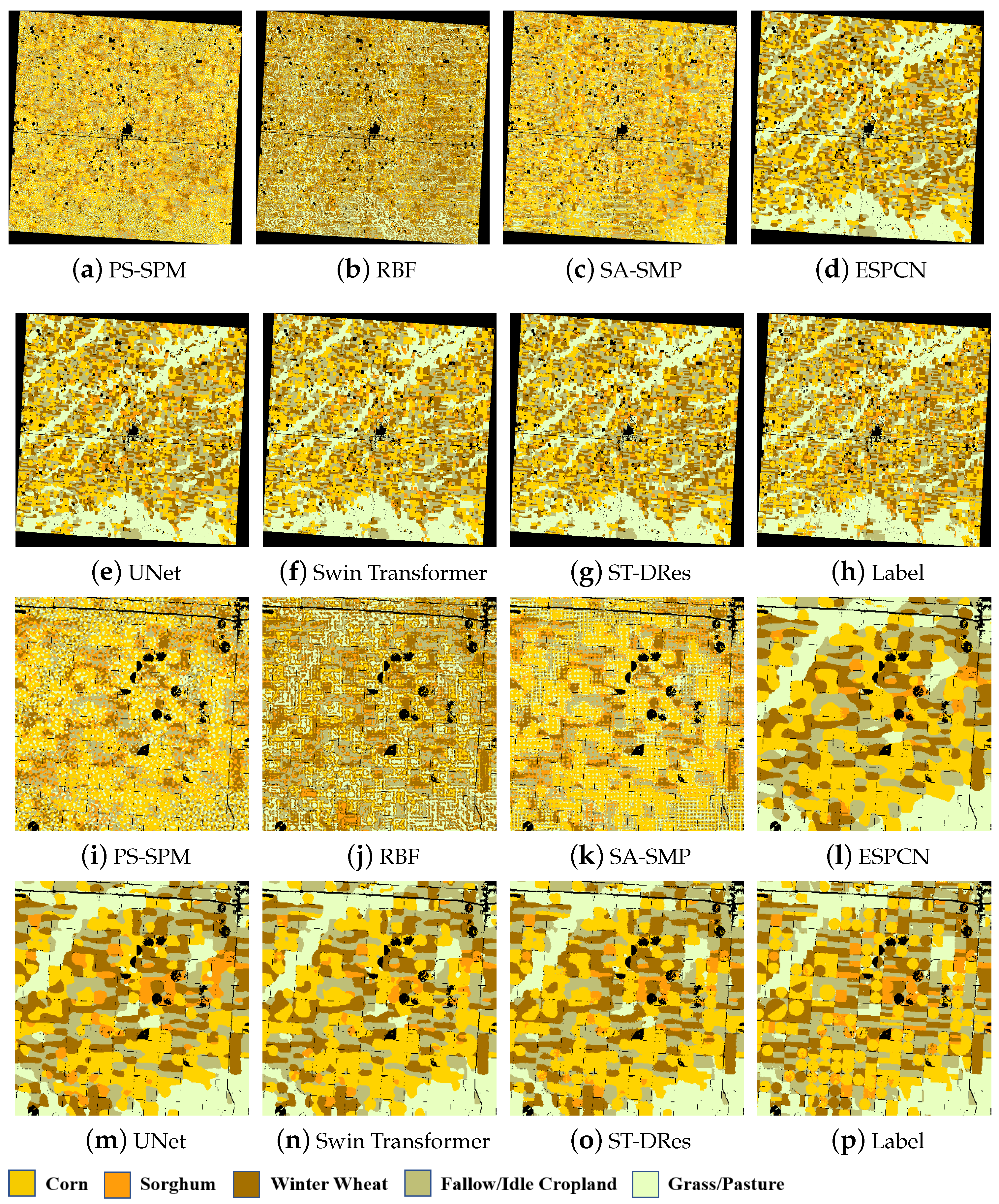
Predicted sub-pixel maps of different methods in Sherman Country in 2017 achieved by different methods. (a–g) show predictions for the entire Sherman County by different methods and (h) is the label map, (i–o) show SPM results for a small example area in Sherman County, and (p) is the corresponding label. Obviously, there are many misclassification pixels in the traditional SPM methods, and ESPCN and UNet networks produce excessively smooth maps. Moreover, the ST-DRes method achieves a good classification result, while Swin Transformer also shows a good result, inferior to ST-DRes only in some details and small classes, such as sorghum.
Figure 4.
Predicted sub-pixel maps of different methods in Sherman Country in 2017 achieved by different methods. (a–g) show predictions for the entire Sherman County by different methods and (h) is the label map, (i–o) show SPM results for a small example area in Sherman County, and (p) is the corresponding label. Obviously, there are many misclassification pixels in the traditional SPM methods, and ESPCN and UNet networks produce excessively smooth maps. Moreover, the ST-DRes method achieves a good classification result, while Swin Transformer also shows a good result, inferior to ST-DRes only in some details and small classes, such as sorghum.
Figure 5.
The optional upsampling architectures at the end of the network.
Figure 5.
The optional upsampling architectures at the end of the network.
Figure 6.
The subfigures (a–e) represent the sub-pixel mapping of five different upsampling methods (nearest, area, bilinear, bicubic and pixelshuffle) implemented on a small portion of the Sherman dataset, including the test accuracy they achieved. And (f) is the corresponding label. It shows that the pixelshuffle layer is more capable of generating sub-pixel maps even in fragmentary parcels and limited crop categories.
Figure 7.
Four small sub-pixel example maps () in the Sherman dataset are displayed by using different temporal and spatial information. (a,e,i) represent the results generated by the three methods (S-DRes,T-DRes, ST-DRes) on example map-1, while (m) is the corresponding label. Similarly, (b,f,j) represent the results generated by the three methods on example map-2, while (n) is the corresponding label; (c,g,k) represent the results generated by the three methods on example map-3, while (o) is the corresponding label; (d,h,l) represent the results generated by the three methods on example map-4, while (p) is the corresponding label. It shows that T-DRes is more capable of generating sub-pixel maps that are closest to the ground truth than S-DRes architecture. ST-DRes outperformed the other two models, which is especially noticeable in the highlighted red box area.
Figure 8.
SPM results of small examples () in different spatial and temporal generalization experiments of different methods are displayed. The rows of “(a) Thomas-2017” and “(b) Gray-2017” represent the results of training in Sherman County in 2017 and testing in Thomas County and Gray County in 2017, respectively. The rows of “(c) Sherman-2018”, “(d) Thomas-2018”, and “(e) McPherson-2018” represent the results of training in Sherman County in 2017 and testing in Sherman County, Thomas Count, and McPherson County in 2018, respectively.
Table 1.
Each class is expressed as an area (km), the number of pixels, and the proportion in Sherman, Thomas, Gray, and McPherson in 2017, respectively.
Table 1.
Each class is expressed as an area (km), the number of pixels, and the proportion in Sherman, Thomas, Gray, and McPherson in 2017, respectively.
| Statistics | County | Corn | Sorghum | Winter Wheat | Fallow | Grass |
|---|
| Pixel Count | Sherman | 684,100 | 174,898 | 640,994 | 616,584 | 758,504 |
| Thomas | 566,438 | 175,689 | 544,659 | 491,250 | 1,119,019 |
| McPherson | 222,513 | 64,398 | 627,134 | 460 | 697,496 |
| Gray | 492,152 | 378,682 | 487,001 | 389,280 | 532,036 |
| Area (km) | Sherman | 615.71 | 157.41 | 576.91 | 554.94 | 682.68 |
| Thomas | 509.81 | 158.13 | 490.21 | 442.14 | 1007.15 |
| McPherson | 200.27 | 57.96 | 564.44 | 0.41 | 627.77 |
| Gray | 442.95 | 340.83 | 438.32 | 350.36 | 478.85 |
| Proportion | Sherman | 22.51% | 5.75% | 21.09% | 20.29% | 24.96% |
| Thomas | 36.18% | 5.68% | 18.31% | 17.61% | 15.88% |
| McPherson | 8.58% | 2.48% | 24.19% | 0.02% | 26.90% |
| Gray | 19.67% | 15.14% | 19.47% | 15.56% | 21.27% |
Table 2.
The accuracy, F1 score of each class, OA, mIoU, and Kappa coefficients of the test sets of different methods (the highest accuracy in each column is in bold).
Table 2.
The accuracy, F1 score of each class, OA, mIoU, and Kappa coefficients of the test sets of different methods (the highest accuracy in each column is in bold).
| Method | Corn | Sorghum | Winter Wheat | Fallow | Grass | OA | mIoU | Kappa |
|---|
| Acc | F1 | Acc | F1 | Acc | F1 | Acc | F1 | Acc | F1 |
|---|
| PS-SMP | 0.6052 | 0.4828 | 0.1762 | 0.0995 | 0.3024 | 0.3765 | 0.3925 | 0.4066 | 0.2348 | 0.2934 | 0.3650 | 0.2765 | 0.3362 |
| RBF | 0.2676 | 0.3267 | 0.0310 | 0.0287 | 0.5368 | 0.3876 | 0.4275 | 0.4547 | 0.3753 | 0.4309 | 0.3766 | 0.2714 | 0.3401 |
| SA-SMP | 0.6576 | 0.5248 | 0.1670 | 0.0943 | 0.3194 | 0.3976 | 0.4359 | 0.4513 | 0.2450 | 0.3062 | 0.3924 | 0.2957 | 0.3649 |
| ESPCN | 0.8315 | 0.7759 | 0.3726 | 0.4413 | 0.7821 | 0.7727 | 0.7483 | 0.7657 | 0.8467 | 0.8625 | 0.7827 | 0.7292 | 0.7588 |
| UNet | 0.8273 | 0.8042 | 0.5458 | 0.5884 | 0.8191 | 0.7914 | 0.7692 | 0.7782 | 0.8598 | 0.8820 | 0.8070 | 0.7701 | 0.7942 |
| Swin Transformer | 0.9045 | 0.8660 | 0.5776 | 0.6775 | 0.8543 | 0.8552 | 0.8531 | 0.8498 | 0.9139 | 0.9231 | 0.8680 | 0.8369 | 0.8443 |
| ST-DRes | 0.9185 | 0.8867 | 0.6405 | 0.7357 | 0.8946 | 0.8802 | 0.8659 | 0.8744 | 0.9267 | 0.9346 | 0.8894 | 0.8639 | 0.8684 |
Table 3.
The train accuracy, train mIoU, test accuracy, test mIoU, predict accuracy, and predict mIoU of the dataset from four kinds of spatial interpolation methods and pixelshuffle layer at the end of the network (the highest accuracy in each column is in bold format.
Table 3.
The train accuracy, train mIoU, test accuracy, test mIoU, predict accuracy, and predict mIoU of the dataset from four kinds of spatial interpolation methods and pixelshuffle layer at the end of the network (the highest accuracy in each column is in bold format.
| Upsample | Train Acc | Train mIoU | Test Acc | Test mIoU | Predict Acc | Predict mIoU |
|---|
| nearest | 0.8411 | 0.8295 | 0.8108 | 0.7726 | 0.7999 | 0.7550 |
| area | 0.8421 | 0.8310 | 0.8145 | 0.7772 | 0.8033 | 0.7570 |
| bilinear | 0.9323 | 0.9231 | 0.8683 | 0.8345 | 0.8521 | 0.8122 |
| bicubic | 0.9272 | 0.9184 | 0.8644 | 0.8319 | 0.8459 | 0.8062 |
| pixelshuffle | 0.9566 | 0.9508 | 0.8784 | 0.8498 | 0.8671 | 0.8337 |
Table 4.
Experimental results of the test dataset from the different temporal channels (
), the number of temporal blocks (
), spatial channel (
), and the number of temporal blocks (
) from the model architecture (
Figure 3). T-DRes indicates that the model uses only temporal blocks. S-DRes indicates that the model uses only spatial blocks. ST-DRes indicates that the model uses both temporal and spatial blocks.
| Method | S Channel | S Block | Train Acc | Train mIoU | Test Acc | Test mIoU |
|---|
| S-DRes | 512 | 1 | 0.8876 | 0.8748 | 0.8471 | 0.8153 |
| S-DRes | 512 | 2 | 0.9287 | 0.9191 | 0.8642 | 0.8336 |
| S-DRes | 512 | 3 | 0.9440 | 0.9357 | 0.8667 | 0.8361 |
| S-DRes | 512 | 4 | 0.9531 | 0.9464 | 0.8670 | 0.8382 |
| S-DRes | 512 | 5 | 0.9558 | 0.9497 | 0.8663 | 0.8352 |
| S-DRes | 512 | 6 | 0.9574 | 0.9513 | 0.8630 | 0.8326 |
| S-DRes | 64 | 4 | 0.8725 | 0.8593 | 0.8327 | 0.7954 |
| S-DRes | 128 | 4 | 0.8978 | 0.8858 | 0.8420 | 0.8080 |
| S-DRes | 256 | 4 | 0.9271 | 0.9165 | 0.8565 | 0.8234 |
| S-DRes | 512 | 4 | 0.9531 | 0.9464 | 0.8670 | 0.8382 |
| S-DRes | 1024 | 4 | 0.9765 | 0.9734 | 0.8779 | 0.8494 |
| Method | T Channel | T Block | Train Acc | Train mIoU | Test Acc | Test mIoU |
| T-DRes | 512 | 1 | 0.7819 | 0.7553 | 0.7640 | 0.7217 |
| T-DRes | 512 | 2 | 0.8319 | 0.8156 | 0.7852 | 0.7479 |
| T-DRes | 512 | 3 | 0.8858 | 0.8702 | 0.8084 | 0.7723 |
| T-DRes | 512 | 4 | 0.8997 | 0.8857 | 0.8154 | 0.7804 |
| T-DRes | 512 | 5 | 0.9229 | 0.9103 | 0.8263 | 0.7917 |
| T-DRes | 512 | 6 | 0.9129 | 0.8999 | 0.8196 | 0.7860 |
| T-DRes | 64 | 5 | 0.8307 | 0.8172 | 0.7808 | 0.7404 |
| T-DRes | 128 | 5 | 0.8843 | 0.8701 | 0.8013 | 0.7659 |
| T-DRes | 256 | 5 | 0.9325 | 0.9205 | 0.8270 | 0.7938 |
| T-DRes | 512 | 5 | 0.9229 | 0.9103 | 0.8263 | 0.7917 |
| T-DRes | 1024 | 5 | 0.7642 | 0.7428 | 0.7550 | 0.7092 |
| Method | S Channel | S Block | T Channel | T Block | Test Acc | Test mIoU |
| ST-DRes | 1024 | 4 | 256 | 5 | 0.8894 | 0.8639 |
Table 5.
The results of different satellite-derived metrics and combinations of reflectance bands for crops SPM.
Table 5.
The results of different satellite-derived metrics and combinations of reflectance bands for crops SPM.
| Input | Train Acc | Train mIoU | Test Acc | Test mIoU | Predict Acc | Predict mIoU |
|---|
| NDVI | 0.9840 | 0.9817 | 0.8893 | 0.8638 | 0.8790 | 0.8524 |
| EVI | 0.9753 | 0.9808 | 0.8744 | 0.8552 | 0.8630 | 0.8436 |
| BRNM | 0.9885 | 0.9826 | 0.8842 | 0.8582 | 0.8806 | 0.8522 |
Table 6.
The accuracy, F1 score of each class, mIoU, OA, and mean mIoU of the test sets of different methods (the highest accuracy in each column is in bold). The table is divided into five sections. The “Thomas-2017” and “Gray-2017” sections represent the results of training in Sherman County in 2017 and testing in Thomas County and Gray County in 2017, respectively. The “Sherman-2018”, “Thomas-2018”, and “McPherson-2018” sections represent the results of training in Sherman County in 2017 and testing in Sherman County, Thomas County, and McPherson County in 2018, respectively.
| Thomas-2017 |
| Method | Corn | Sorghum | Winter Wheat | Fallow | Grass | OA | mIoU |
| Acc | F1 | Acc | F1 | Acc | F1 | Acc | F1 | Acc | F1 |
| ESPCN | 0.7741 | 0.7594 | 0.2841 | 0.3194 | 0.6706 | 0.6589 | 0.6001 | 0.6498 | 0.7453 | 0.6952 | 0.6924 | 0.6165 |
| UNet | 0.6310 | 0.7112 | 0.4338 | 0.3767 | 0.6794 | 0.6401 | 0.7532 | 0.6606 | 0.7195 | 0.7119 | 0.6669 | 0.6201 |
| Swin Transformer | 0.7561 | 0.7608 | 0.3663 | 0.4015 | 0.6662 | 0.6490 | 0.6502 | 0.6607 | 0.7460 | 0.7179 | 0.6992 | 0.6380 |
| ST-DRes | 0.7831 | 0.7727 | 0.3286 | 0.3986 | 0.6597 | 0.6577 | 0.6569 | 0.6640 | 0.7588 | 0.7251 | 0.7096 | 0.6436 |
| Gray-2017 |
| Method | Corn | Sorghum | Winter Wheat | Fallow | Grass | OA | mIoU |
| Acc | F1 | Acc | F1 | Acc | F1 | Acc | F1 | Acc | F1 |
| ESPCN | 0.5014 | 0.4166 | 0.1593 | 0.2259 | 0.5859 | 0.5611 | 0.5055 | 0.4926 | 0.6461 | 0.6050 | 0.5132 | 0.4602 |
| UNet | 0.4752 | 0.3934 | 0.2111 | 0.2886 | 0.5686 | 0.5411 | 0.5703 | 0.4922 | 0.6179 | 0.5939 | 0.4949 | 0.4618 |
| Swin Transformer | 0.5828 | 0.4795 | 0.2211 | 0.2955 | 0.5684 | 0.5387 | 0.5422 | 0.4830 | 0.5707 | 0.6188 | 0.5251 | 0.4831 |
| ST-DRes | 0.5462 | 0.4856 | 0.2329 | 0.3177 | 0.6050 | 0.5479 | 0.5396 | 0.4990 | 0.6173 | 0.6363 | 0.5418 | 0.4973 |
| Sherman-2018 |
| Method | Corn | Sorghum | Winter Wheat | Fallow | Grass | OA | mIoU |
| Acc | F1 | Acc | F1 | Acc | F1 | Acc | F1 | Acc | F1 |
| ESPCN | 0.6743 | 0.6597 | 0.0399 | 0.0643 | 0.5045 | 0.6264 | 0.6891 | 0.7139 | 0.8566 | 0.6530 | 0.6589 | 0.5435 |
| UNet | 0.6783 | 0.6926 | 0.2997 | 0.2928 | 0.7052 | 0.6951 | 0.7879 | 0.6766 | 0.6379 | 0.6875 | 0.6831 | 0.6089 |
| Swin Transformer | 0.6382 | 0.6669 | 0.0700 | 0.1133 | 0.6711 | 0.5730 | 0.8051 | 0.6176 | 0.3826 | 0.4978 | 0.6001 | 0.4937 |
| ST-DRes | 0.6685 | 0.6891 | 0.0518 | 0.0802 | 0.6621 | 0.6962 | 0.6564 | 0.6425 | 0.8393 | 0.7182 | 0.6862 | 0.5653 |
| Thomas-2018 |
| Method | Corn | Sorghum | Winter Wheat | Fallow | Grass | OA | mIoU |
| Acc | F1 | Acc | F1 | Acc | F1 | Acc | F1 | Acc | F1 |
| ESPCN | 0.7857 | 0.7116 | 0.0377 | 0.0534 | 0.4248 | 0.5425 | 0.5264 | 0.5664 | 0.6813 | 0.5438 | 0.6131 | 0.4835 |
| UNet | 0.5608 | 0.6473 | 0.3409 | 0.2987 | 0.6318 | 0.6058 | 0.7388 | 0.5422 | 0.4359 | 0.4438 | 0.5664 | 0.5076 |
| Swin Transformer | 0.7617 | 0.7158 | 0.0262 | 0.0446 | 0.4640 | 0.5127 | 0.7898 | 0.4960 | 0.2017 | 0.3101 | 0.5686 | 0.4159 |
| ST-DRes | 0.7561 | 0.7214 | 0.0306 | 0.0498 | 0.5583 | 0.6221 | 0.4690 | 0.5063 | 0.7271 | 0.5866 | 0.6335 | 0.4972 |
| McPherson-2018 |
| Method | Corn | Sorghum | Winter Wheat | Fallow | Grass | OA | mIoU |
| Acc | F1 | Acc | F1 | Acc | F1 | Acc | F1 | Acc | F1 |
| ESPCN | 0.3833 | 0.3389 | 0.2338 | 0.2186 | 0.1765 | 0.2802 | 0.1752 | 0.0006 | 0.6803 | 0.6172 | 0.4631 | 0.2911 |
| UNet | 0.4248 | 0.2942 | 0.0000 | 0.0000 | 0.5355 | 0.6220 | 0.1910 | 0.0007 | 0.6415 | 0.6372 | 0.5610 | 0.3108 |
| Swin Transformer | 0.0937 | 0.1604 | 0.4518 | 0.3625 | 0.8594 | 0.7004 | 0.0125 | 0.0040 | 0.4192 | 0.4688 | 0.6271 | 0.3392 |
| ST-DRes | 0.1473 | 0.2323 | 0.3217 | 0.3364 | 0.8341 | 0.7409 | 0.0111 | 0.0055 | 0.6071 | 0.5901 | 0.6872 | 0.3810 |

 ,
, 


