Individual Tree Detection in Coal Mine Afforestation Area Based on Improved Faster RCNN in UAV RGB Images

Abstract

Forests are the most important part of terrestrial ecosystems. In the context of China’s industrialization and urbanization, mining activities have caused huge damage to the forest ecology. In the Ulan Mulun River Basin (Ordos, China), afforestation is standard method for reclamation of coal mine degraded land. In order to understand, manage and utilize forests, it is necessary to collect local mining area’s tree information. This paper proposed an improved Faster R-CNN model to identify individual trees. There were three major improved parts in this model. First, the model applied supervised multi-policy data augmentation (DA) to address the unmanned aerial vehicle (UAV) sample label size imbalance phenomenon. Second, we proposed Dense Enhance Feature Pyramid Network (DE-FPN) to improve the detection accuracy of small sample. Third, we modified the state-of-the-art Alpha Intersection over Union (Alpha-IoU) loss function. In the regression stage, this part effectively improved the bounding box accuracy. Compared with the original model, the improved model had the faster effect and higher accuracy. The result shows that the data augmentation strategy increased AP by 1.26%, DE-FPN increased AP by 2.82%, and the improved Alpha-IoU increased AP by 2.60%. Compared with popular target detection algorithms, our improved Faster R-CNN algorithm had the highest accuracy for tree detection in mining areas. AP was 89.89%. It also had a good generalization, and it can accurately identify trees in a complex background. Our algorithm detected correct trees accounted for 91.61%. In the surrounding area of coal mines, the higher the stand density is, the smaller the remote sensing index value is. Remote sensing indices included Green Leaf Index (GLI), Red Green Blue Vegetation Index (RGBVI), Visible Atmospheric Resistance Index (VARI), and Normalized Green Red Difference Index (NGRDI). In the drone zone, the western area of Bulianta Coal Mine (Area A) had the highest stand density, which was 203.95 trees ha⁻¹. GLI mean value was 0.09, RGBVI mean value was 0.17, VARI mean value was 0.04, and NGRDI mean value was 0.04. The southern area of Bulianta Coal Mine (Area D) was 105.09 trees ha⁻¹ of stand density. Four remote sensing indices were all the highest. GLI mean value was 0.15, RGBVI mean value was 0.43, VARI mean value was 0.12, and NGRDI mean value was 0.09. This study provided a sustainable development theoretical guidance for the Ulan Mulun River Basin. It is crucial information for local ecological environment and economic development.

1. Introduction

Vegetation covers approximately 70% of the Earth’s land surface. It is one of the most important components of ecosystems [1]. Forest has higher levels of multiple ecosystem services value than grassland [2]. Trees can alleviate ecological problems caused by liquefied petroleum fuels, industrialization, and coal burning. In ecological restoration area, the forest requires little maintenance. It can create stable nutrient cycles, energy flows, feedback loops, and biodiversity. In surface ecosystems, forests can increase landscape diversity, enhance landscape connectivity, and accelerate soil renewal [3]. Forest can also improve the soil quality [4]. For example, it increases effectively the organic matter content of the topsoil [5]. In the local carbon cycle, forests supplement the sequestration potential of depleted carbon dioxide [6]. They store carbon in the xylem, root system and mycorrhiza. It also creates suitable soil condition [7]. Under the influence of coal mining and urbanization [8], forest ecosystem was affected seriously [9]. The ecological restoration project of the damaged coal mine areas include soil backfill and afforestation. However, the backfill soil and the original soil are different; the tree growth situations were different [10]. In order to reduce the environment pollution, the Ministry of Natural Resources of China issued an opinion to incorporate mine ecological restoration planning into the national land and space planning system in 2019 [11]. Vegetation information, such as tree location and canopy condition [12], is critical in local mine ecological restoration. Traditional tree management in mining recovery area consists of three steps: dividing the forest into different sections, selecting different tree species in each random room, and manual investigation of tree growth [13]. This is a time-consuming and labor-intensive work [14]. The obtained sample number is small.

The opening of low-altitude airspace has changed traditional research methods. In recent years, UAV technology has great progress. In the ecological environment application, UAV remote sensing provides an efficient way to collect large-area surface information [15]. It is also used widely in forestry [16] resource surveys [17]. Zarco-Tejada et al. used fluorescence, temperature, and narrowband indices acquired by an unmanned aerial vehicle platform to detect water stress [18]. Popular UAV forestry applications are plant identification [19], invasive species detection [20], canopy detection [21], and vegetation disease monitoring [22]. Wallace et al. used a UAV lidar system in forest ecosystem [23]. Feng et al. performed urban vegetation mapping with UAV remote sensing [24]. Sferlazza et al. used UAV to study the basal area of virgin forests [25]. UAV multi-temporal images could analysis riparian forest species classification and health [26]. Qiu et al. proposed a new individual tree crown delineation method [27]. Steven et al. used machine learning methods to classify deciduous tree species [28]. These studies provided convenient [29] monitoring methods for forests [30,31,32]. It guides the forest ecological policy effectively in the mining area. How to locate tree accurately in remote sensing image is the key point in UAV applications.

The development of deep learning (DL) provides a solution to this problem. Target detection algorithms have been one of the core problems of computer vision [33]. The goal is to find all regions of interest (ROIs) in the image. Then determine their category. Trees have different appearances, different shapes, and poses in drone images. These are affected by lighting condition and material coverage. These problems can make smaller trees more difficult to detect [34]. There are two main kinds of target detection algorithms. The main difference between these is whether they can generate a regional proposal network. Ross Girshick first proposed the two-stage R-CNN [35] in 2014. Subsequent developments are SPP-Net [36], MR-CNN [37], Fast R-CNN [38], and Faster R-CNN [39]. One-stage has YOLOv1 [40], YOLOv2 [41], YOLOv4 [42], SSD [43], RetinaNet [44], FCOS [45], etc. Lin et al. applied the Feature Pyramid Networks (FPN) [46] to solve small objective detection problems. In 2019, Guo et al. [47] proposed AugFPN to decrease the semantic gap between features at different stages. Qiao et al. proposed the recursive FPN structure in 2020 [48]. This kind of structure increased global features and perceptual fields. Zhang et al. proposed [49] the D-FPN structure in 2021, improving the feature extraction capability of the Faster R-CNN. However, these methods do not take into account the range distribution of the label in the feature extraction process. The scale imbalance and spatial imbalance exist in small targets. This will affect the final training results. In addition, the up-sampling process in FPN of these methods is relatively simple. Important information in the image may be lost. The hierarchical feature extraction function of feature network inevitably leads to the compression of small elements. At higher convolution stage, the model easily blends small objects with the background. These shortcomings make it difficult to detect young trees. FPN [46] provides a lateral path connection to fuse multi-scale features. PANet [50] performed a secondary fusion on FPN, and Bi-FPN [51] added cross-scale connectivity to PANet. However, these structures reduce the presence of low-level features. To solve these problems, we proposed an improved Faster R-CNN model. This paper makes the following contributions:

Multi-strategy fusion data augmentation is used to balance bounding boxes;

DE-FPN structure is developed for image feature extraction;

Modified generalized function is used in the regression stage to improve the detection accuracy.

This paper organized as follows. In Section 2, it shows the study area and the improved Faster R-CNN model. In Section 3, it shows the results of the model experiments. Section 4 and Section 5 are the discussion and conclusion sections, respectively.

2. Data and Method

2.1. Study Area

The Ulan Mulun River Basin locates in the southeast region of Ordos, China (Figure 1). The river originated from the desert area of Ikezhao League [52]. The Ulan Mulun River’s length is 132.5 km and drainage area is 6375 square kilometers. The longitude of the basin ranges from 109.98° to 110.28°E and the latitude ranges from 39.27° to 39.42°N [53]. It belongs to the north temperate arid continental climate. The annual average temperature was 6.2 °C. The precipitation [54] is mainly concentrated in July, August and September. The precipitation accounted for about 70% of the annual precipitation. The Ulan Mulun River Basin is an important energy base in the Ordos [55]. In the middle of the sub-basin is the world’s largest single-well mine, the Bulianta Coal Mine. The recoverable reserves are 1.224 billion tons, and the coal field area is 106.43 square kilometers [52]. See Figure 1 for the location.

2.2. Data

The experimental data was captured by UAV. Flight areas show in Figure 1a–d. The green box represents the training dataset region, and the gray box represents the validation dataset region. The four flight areas named as Area A, Area B, Area C, and Area D, respectively. Area A located in the western region of the Bulianta Coal Mine. Area B was far from the Bulianta Coal Mine. Area C located in the northwestern region of the coal mine. Area D located in the southern region of the coal mine. DJI Phantom 4 Multispectral (P4M) UAV acquired images in August 2021. The weather was cloudless with an excellent atmospheric window. P4M sensor included 6 × 1/2.9″ CMOS. One color sensor for RGB imaging and 5 monochrome sensors for multispectral imaging. Lenses could record solar irradiance automatically to compensate light. It could replace whiteboard calibration. This study mainly used a color sensor lens of RGB. UAV images calibrated procedures as follows: keypoints extraction, keypoints matching, camera model optimization, GPS/GCP geolocation, 3D texture mesh creation, digital surface model creation, orthomosaic creation, reflectance map creation, and index map creation. These processes produced four large-scale composite images. Then we cropped for 576 images by Python [54]. The expert made labels by LabelImage in PascalVOC format. Label shows in Figure 1c,d. Other parameters are shown in

Table 1. DJI P4M parameters.

Parameters	Value
Individual sensors total pixels	2.12 million
Individual sensors effective pixels	2.08 million
FOV	62.7°
Focal length	5.74 mm
Aperture	f/2.2
Average ground sampling distance	5 m
Spatial resolution	0.01 m
Flight time	10:00 A.M.–15:00 P.M.
Flight height	30 m

.

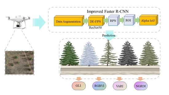
2.3. Improved Faster R-CNN Framework

The Faster R-CNN achieved end-to-end object detection [56]. The algorithm structure showed in Figure 2. Main structure included 4 parts, feature extraction module, Region Proposal Networks (RPN), Region of Interesting Pooling (ROI Pooling), and classification. The feature extraction module was light green, RPN was dark green, ROI Pooling was light cyan, and classification was light pink. First, the image was fed into the feature extraction network. The high-dimensional feature map was extracted through the deep learning convolutional neural network. Second, abstract data flow into the RPN structure [57]. RPN computed the approximate object bounding box location. After the feature map through a 3 × 3 convolutional layer and an activation function, there were two 1 × 1 convolutional paths. One of the paths went through two reshape operations and one softmax judgment. Another path connected a 1 × 1 boosted dimensional convolution kernel and a simple two-category judgment. RPN used bounding box regression to correct the anchor location. In ROI Pooling [58], information filled into subsequent fully connected layers. In the classification and regression module, the algorithm determined the final object bounding box through proposal and feature map. The dark pink area was the innovation of our proposal. The programming language was python3.6, and the deep learning framework was pytorch1.5.

2.4. Multi-Strategy Fusion Data Augmentation

The drone image size was 1600 × 1300. In the training dataset, all labels were divided into 5 classes. This was based on the size of the detection frame. These five categories were 0–100, 101–200, 201–300, 301–400, 401–1000. The statistical results of the labeled dataset of UAV images showed in Figure 3a. The first four categories ranged from 0 to 400, accounting for 98.88%. There was an obvious problem of sample feature imbalance. We used data augmentation based multi-strategy fusion to balance the bounding boxes. In the first step, we cropped the image and blended the patches [59] to form new sample data. In the second step, random erasing [60] was performed. We masked image with gray blocks or Gaussian noise. Noise could reduce overfitting during training and improve generalization performance. In the third step, we put images into the generative adversarial network (DAGAN) [61] to generate new samples. In the final step, the expert marked acquired samples. We ensured that the sample number varied by no more than 10%. These methods compensated for the irrationality of large data samples. The workflow showed in Figure 3b.

2.5. DE-FPN Structure

Feature pyramid networks have excellent performance in building hierarchical representations. We designed the dense enhance FPN (DE FPN) structure. The DE-FPN structure was shown in Figure 4a. DE-FPN not concatenated feature maps directly into the FPN structure. Convolution operations were used to enhance hierarchical features before the data stream into the FPN. {C2 C3 C4 C5} had {4 3 2 1} convolutional layers, respectively. These operations balanced the differences between abstract features. Padding and the stride were 1. We developed multiscale dilated convolution (MDC) in up-sampling in Figure 4b. MDC dilated the convolution with four different dilation factors. By traversing all modes of each filter, it formed a convolutional array of fused features. MDC enriched the sampling pattern in up-sampling. The Dilation Convolution Module (DCM) included three dilated convolution operations. The dilation rates were 1, 2, and 3, respectively. The F-layer features fused with the P-layer image features. Global Context Block (GCB) provided learnable semantic fusion between different layers. We designed the Feature Pyramid Network to improve detection accuracy by GCB [62]. The convolutional layers connected the P-layers by DCM. The convolutional layer connected the F-layers by GCB. Convolution layers connected to other F-layers by MDC. The F-layers performed MDC in the up-sampling connection. High-level semantic information fused in the F and P layers. This structure generated global features in each layer via GCB. It established effective long-range dependencies. It reduced the gap of large semantics. At the same time, the P information layer had the advantage of multiple receptive fields.

2.6. Modified Generalized Function

In the Faster R-CNN regression detection stage, IoU loss function was main part. In this study, we abandoned the conventional narrow IoU loss function, and we used the generalized function Alpha-IoU [63]. The Alpha-IoU loss function used the Box-Cox transformation, and the parameter α obtained by the maximum likelihood method. In the first step, it computed ${\mathrm{Z}}_{\mathrm{i}}^{\left(\mathsf{\alpha }\right)}$ and introduced the Jacobi determinant. In the second step, it needs to calculate its residual sum of squares. Third, repeated these steps. We used the alpha curve to acquire the minimum value. The fourth step calculated $\hat{\mathsf{\beta }}(\hat{\mathsf{\alpha }})$, where P represented the regularization term. He et al. [63] applied a simplified ${ℒ}_{\mathsf{\alpha }-\mathrm{IoU}}=1-{\mathrm{IoU}}^{\mathsf{\alpha }}$ formulation in object detection research. Considering the generality of the indicator, we adopted the original formula. Replaced ${\mathsf{\alpha }}_1$ with ${\mathsf{\alpha }}_1+\frac{1}{{\mathsf{\alpha }}_1}$. An inverse function was added in the exponent term to minimize the minimum closed convexity.

$${ℒ}_{\mathsf{\alpha }-\mathrm{IoU}}=\frac{(1-{\mathrm{IoU}}^{{\mathsf{\alpha }}_1+\frac{1}{{\mathsf{\alpha }}_1}})}{{\mathsf{\alpha }}_1+\frac{1}{{\mathsf{\alpha }}_1}}+{\mathrm{P}}^{{\mathsf{\alpha }}_2}\left(\mathrm{B},{\mathrm{B}}^{\mathrm{gt}}\right),{\mathsf{\alpha }}_1,{\mathsf{\alpha }}_2\ge 0,$$

(1)

Alpha-IoU improved the bounding box regression accuracy with adaptive reweighting. When α was between (0, 1). It reduced localization accuracy and produced poorly performing detection frames. α was closely related to the size of the loss function. He et al. [63] suggested α equal to 3. We tested the value of α on the UAV dataset. The result showed that the object detection model performed better when α was 2.7. We set a multi-stage IoU [64] threshold of (0.5, 0.6, 0.7). The weight of each stage set to (0.75, 1, 0.25) [65].

2.7. Hyperparameters and Backbone

The learning rate was 0.0001, the weight decay coefficient was 0.0005, and the learning decay rate was 0.1. We used a linear decay function. It became one-tenth of its original value after a fixed period. We trained the model on a virtual machine with an NVIDIA Tesla V100 GPU. GRID driver version was 470.57.02, the CUDA version was 11.4 and it had 32 G RAM. The operating system was Ubuntu 18.04, and the framework was Pytorch 1.9.

We tested seven backbone models, VGG11, VGG16, VGG19 [66], ResNet18, ResNet34, ResNet50 [67] and MobileNetV2 [68]. In VGGNet, four full connection layers were removed and the parameters of the first two layers frozen. In the ResNet model, we frozen the first convolutional layer and the first basic block structure. We opened the rest of the network for forwarding and backward propagation. Two IR layers frozen. Dropout and linear layers were removed in MobileNet V2. These networks all used transfer learning to initialize the pre-training parameters. The transfer learning dataset was the ImageNet dataset.

2.8. Aerial Photography Area

In Equation (2), H is the flight height, ƒ is the focal length of the camera lens [69], GSD is the ground resolution, and a is the pixel size. This formula can be used to calculate the surface area in an UAV image. If we sum up all the trees in the image, we can acquire the total number of trees in the flight area. Further, we can estimate the stand density in four areas.

H = (ƒ × GSD)/a,

(2)

2.9. Remote Sensing Indexes

We applied orthorectification correction by Pix4d mapper and computed remote sensing indexes. It is convenient to achieve vegetation information extraction from UAV images. G is the green band, R is the red band, and B is the blue band.

The GLI [70] is an alternative index to the NDVI. It shows in Equation (3).

GLI = (G − R + G − R)/(G + R + G + R),

(3)

RGBVI [71] is an unsupervised classification method to classify vegetation from other land covers. It shows in Equation (4).

RGBVI = (G × G − R × B)/(G × G + R + B),

(4)

VARI [72] shows in Equation (5)

VARI = (G − R)/(G + R − B),

(5)

NGRDI [73] is a normalization index that consisting green band and red band. It shows in Equation (6)

NGRDI = (G − R)/(G + R),

(6)

3. Results

3.1. Modules Effectiveness Evaluation

Ablation experiment results are shown in

Table A1. AP values of different Backbone and improved methods in Faster R-CNN.

Backbone	DA	DE-FPN	Alpha-IoU	AP	AP50	AP60	AP70
VGG11				71.54	77.70	74.59	40.87
	√			71.94	79.31	74.04	41.36
		√		75.16	84.22	74.94	48.89
			√	71.63	79.64	73.87	38.66
	√	√		74.74	84.17	75.17	44.74
		√	√	72.18	81.18	73.21	41.09
	√		√	74.25	80.76	77.56	41.45
	√	√	√	75.85	86.52	75.53	45.13
VGG16				73.27	85.27	72.11	41.88
	√			75.76	86.84	76.28	40.45
		√		73.94	83.49	75.02	40.92
			√	73.98	89.43	70.68	40.84
	√	√		76.81	90.83	72.11	53.55
		√	√	74.71	87.79	71.54	48.16
	√		√	75.75	89.55	74.27	40.30
	√	√	√	77.65	97.77	70.15	47.27
VGG19				75.07	87.94	70.47	54.88
	√			76.70	88.41	75.82	45.09
		√		74.89	90.99	70.80	42.95
			√	73.89	87.76	70.69	45.07
	√	√		76.14	94.92	71.04	40.19
		√	√	77.53	97.86	71.63	40.14
	√		√	76.40	91.58	71.93	48.78
	√	√	√	78.29	88.92	77.65	48.96
ResNet18				75.03	85.69	72.99	51.22
	√			75.40	86.95	72.60	51.93
		√		72.89	84.85	70.91	44.99
			√	79.76	94.11	75.56	53.48
	√	√		75.42	86.43	71.39	58.54
		√	√	80.07	90.98	77.33	58.24
	√		√	80.26	92.26	79.90	45.64
	√	√	√	80.80	90.57	80.23	53.77
ResNet34				71.87	82.19	69.90	48.77
	√			74.64	89.13	70.87	46.28
		√		76.15	87.90	72.92	53.82
			√	75.92	84.82	76.38	47.33
	√	√		78.23	87.79	79.55	44.29
		√	√	76.53	86.40	75.22	52.11
	√		√	73.84	84.44	73.08	45.09
	√	√	√	79.58	87.83	81.62	46.66
ResNet50				81.93	93.66	81.20	49.61
	√			83.18	96.18	82.49	46.98
		√		84.50	93.99	84.34	56.68
			√	84.53	91.04	86.60	56.68
	√	√		82.11	91.43	80.93	58.87
		√	√	83.77	93.21	84.19	53.78
	√		√	86.70	94.64	87.72	58.78
	√	√	√	89.89	98.93	90.43	60.60
MobileNet V2				56.37	70.76	52.28	29.58
	√			56.82	71.18	52.75	30.01
		√		58.29	72.93	53.41	33.88
			√	58.74	72.61	53.41	38.44
	√	√		59.18	72.55	55.11	35.38
		√	√	58.65	71.72	54.12	37.57
	√		√	59.85	73.65	55.86	34.39
	√	√	√	60.78	74.05	56.96	36.26

. The result showed that three improvements can improve the target detection accuracy. In multi-strategy image augmentation, ResNet34 showed the most significant increase 2.78% in AP, while VGGNet11 only increased by 0.39%. The best backbone network was ResNet34 with DE FPN strategy, which increased by 4.28%. However, in ResNet18, AP decreased by 2.13%. In the improved Alpha-IoU result, ResNet18 performed best, with an AP increase of 4.73%. Among the dual improvement combinations, the most significant AP improvements are multi-strategy image enhancement and DE FPN. It increased by 6.37% in ResNet34. The combination of DE FPN and Alpha-IoU showed the most significant improvement in ResNet18. It was 5.04%. The most significant AP improvement among the three strategies is ResNet50. It increased to 89.89%. It showed that among seven backbone networks, ResNet50 was the best backbone. The tree detection accuracy was the highest, and the detection error was the smallest.

We compared the training curve and the loss rate curve (The top half of Figure 5). The detection result graph showed in the upper part of Figure 5. It could be seen that the loss rate decreases gradually as the number of epochs increased. After 15 epochs, the overall learning rate stabilized. The ResNet had a lower overall loss rate than the MobileNet V2 and VGGNet. The possible reason was the advantage of the residual structure. The loss rate of VGGNet11 was the largest among the 7 models. The value was 0.86. ResNet50 had the lowest loss rate of 0.41. It was 0.45 lower than VGGNet11.

Figure 5a–g showed the detection result of tree in the UAV RGB image. These areas were planted woods. Overall, most of the trees were successfully detected. Green boxes represented the tree detection result. In Figure 5d, MobileNet V2 had the problem of overlapping detection frames. In Figure 5g, ResNet50 detected two trees at the edge of the red box, which was not captured by the other models. We concluded that Faster R-CNN had the best performance when ResNet50 was backbone. This model had the best learning ability and comprehensive tree detection result.

In the coal mine area, young tree had a shape that closed to low shrubs. Some mature trees had overlapping crowns. It brought certain difficulties to the target detection model. In order to test the detection algorithm performance under extreme conditions, we selected two UAV images for experiment. Figure 6(1-a) was a low tree image, which was very similar to surface shrubs in appearance. Figure 6(2-a) was an image that canopy overlaid with trees and shadows. In the scene of low trees, ResNet50 localized all the trees accurately and did not overlap the detection box. Other methods were less able to detect incomplete trees. Such as four small trees in the upper left corner of the image. MobileNet V2 and ResNet18 misidentified bushes. In Figure 6(2-a), ResNet50 had excellent performance in tree recognition. The identification result of VGG11, VGG16, MobileNet V2, ResNet18 and ResNet34 had certain flaws. The detection frame was only located in a partial area of the tree, and not detected the complete tree. VGG19 exaggerated the tree detection range in shaded areas.

3.2. Module Evaluation

In this part, we used ResNet50 as the backbone network. It was important to further test model performance with popular method. The result showed in

Table 2. Improved module evaluation.

	Method	ΔAP
DA	RE	0.16
	RIC	0.31
	DAGAN	0.82
	RE + RIC + DAGAN	1.26
FPN	EnFPN	1.99
	AugFPN	2.13
	iFPN	2.44
	DE-FPN	2.82
IoU Loss	DIoU	1.33
	GIoU	0.82
	CIoU	2.21
	Alpha-IoU	2.60

ΔAP means the variation of AP.

. RE was the abbreviation of the Random Erasing [60], and RIC was the abbreviation of Random Image Cropping [59]. Deep Learning DAGAN was superior to geometric data enhancement. DAGAN [74] improved AP by 0.82. The combination of deep learning and traditional data enhancement technique improved detection accuracy. The experimental result also proved the effectiveness of the multi-strategy data enhancement method. The FPN structure bridged the gap of insufficient semantic information in the detection process [46]. In the FPN comparison experiment, we tested several other FPN variants on tree. There were EnFPN [75], AugFPN [76] and iFPN [77]. It showed that UAV image feature extraction was the core process, DE-FPN could obtain more valuable semantic information. The DE-FPN focused more on the tree’s high-dimensional features and enhanced generalization. In the loss function section, we compared it with mainstream target detection loss functions. There were DIoU [78], GIoU [79] and CIoU [80]. In the mining tree dataset, GIoU had the lowest accuracy, and our improved Alpha-IoU contributed 1.78% more. The results showed in Table 2.

3.3. Accuracy Comparison with Other Models

We compared the improved Faster R-CNN with some mainstream target detection models. The backbone was ResNet50. The experiment focused on the impact of different algorithmic design structures. The test dataset was all labeled UAV images. The results showed in

Table 3. Target detection model comparison.

Model	Backbone	AP	AP50	AP60	AP70
Faster R-CNN	ResNet50	89.89	98.93	90.43	60.60
Mask R-CNN [81]	ResNet50	81.42	87.76	82.26	59.04
TridentNet [82]	ResNet50	79.70	81.25	85.89	50.27
YOLO v3 [83]	DarkNet-53	85.18	90.47	89.51	52.02
YOLO v4 [84]	CSPDarkNet-53	78.85	82.93	81.84	54.67
YOLO v5 [85]	ResNet50	83.89	93.58	84.77	51.29
SSD [86]	ResNet50	82.24	90.25	83.54	52.99
FCOS [87]	ResNet50	83.71	92.43	85.46	50.55
CenterNet511 [88]	Hourglass104	84.66	91.00	87.32	55.02
EFLDet [59]	BRNet-ResNet50	86.08	90.38	89.83	58.17
DETR [89]	ResNet50	86.06	94.74	86.63	58.73
ViDT [90]	ViT	85.67	91.28	88.29	58.39

. Overall, as the score threshold increased gradually from 50 to 70, the algorithms showed a decreasing trend of AP. The model robustness enhanced. As the feature screening threshold raised, it would increase the identifying difficulty of the ROI area. The results showed that the improved Faster R-CNN outperformed other models. It was 8.47% higher than the Mask R-CNN model and 5.23% higher than the anchorless one-stage detection model CenterNet511. The AP of the improved Faster R-CNN was 6% higher than that of YOLO v5. AP₆₀ was 9.31% higher than that of YOLO v5. In the transformer, we chosen DETR and ViDT. The improved Faster R-CNN had an increase of 3.83% and 4.22%, respectively.

The AP comparison result showed that the improved Fast R-CNN and EFLDet have the first and second precision in the 9 algorithms, respectively. In order to test the generalization performance of the two algorithms, we selected a drone image with a large number of trees. The results showed in Figure 7. The flying height of the drone was 50 m. It can be found that there are 7 undetected trees for the two algorithms. Blue box represented undetected trees. Missing trees accounted for 8.3% of the total. Improved Faster R-CNN detected correct trees accounted for 91.61% of the total, while EFLDet only accounted for 59.52%. It showed that the improved Faster R-CNN algorithm has better generalization in detecting trees in mining areas.

3.4. Stand Density

To apply the improved algorithm in practice, we also designed a counting system. In the upper left corner of the UAV image, program marked the statistical result of the detected tree (Figure 8). After batch processing, improved Faster R-CNN identified and counted trees in all images. Same tree in adjacent images had been removed. When the flight height was 30 m, the GSD value of P4M was 1.5873 cm/pixel. A single image field length was 1600 × GSD/100 = 25.3968 m. The field width was 1300 × GSD/100 = 20.6349 m. It could be calculated that the shooting area was about 524 square meters. Then we calculated stand density. The results showed in

Table 4. Stand Density in UAV images of four region.

	A	B	C	D
Number of Tree	1539	971	602	793
Area (ha)	7.546	7.546	7.546	7.546
Stand Density (trees ha−1)	203.95	128.68	79.78	105.09

. Area A had the largest number trees at 1539, and area C had the fewest trees at 602. The density was the tree number divided by corresponding experimental area. Area A was 203.95 trees ha⁻¹. Area C was 79.78 trees ha⁻¹. The order of stand density was A > B > D > C.

3.5. Remote Sensing Indices Results

Remote sensing indices could eliminate tree shading and highlight the shape of the canopy. In Figure 9, the dark blue areas were bare ground. The red and yellow were vegetation. Remote sensing indices of the trees and grassland had obvious variability. The tree average remote sensing indices in the bounding box were calculated as the quantitative remote sensing actual value for a single tree. We took this value into subsequent calculations. The tree GLI index was distributed between 0.06 and 0.22. Bare ground value was below the 0.01, and grassland value was between 0.01 and 0.10 generally. In the RGBVI, tree values were generally between 0.16 and 0.77. It had a wide range of variation. Bare ground values were below 0.10. Grassland values were between 0.10 and 0.20. The VARI index provided lower values for the tree, it was between 0.01 and 0.25. Negative values were in bare ground and grassland. The value of grassland was greater than that of bare land. The tree’s NGRDI index ranged from 0.02 to 0.19. The numerical characteristics of bare ground and grassland were similar in the VARI index.

We calculated remote sensing index for all trees in the imagery. Duplicate trees had removed in adjacent images.

Table 5. Remote sensing indexes results of trees in UAV images of four region.

		GLI	RGBVI	VARI	NGRDI
A	Min	0.06	0.16	0.02	0.03
	Max	0.15	0.22	0.06	0.05
	Mean	0.09	0.17	0.04	0.04
B	Min	0.07	0.21	0.01	0.02
	Max	0.17	0.49	0.08	0.07
	Mean	0.10	0.27	0.05	0.05
C	Min	0.07	0.16	0.01	0.02
	Max	0.16	0.51	0.12	0.18
	Mean	0.12	0.34	0.07	0.08
D	Min	0.06	0.21	0.02	0.03
	Max	0.22	0.77	0.25	0.19
	Mean	0.15	0.43	0.12	0.09

showed the statistical results of the four remote sensing indices. Area A had the smallest GLI mean value at 0.09. Area D had the largest GLI mean value at 0.15. The mean value of GLI was D, C, B and A in descending order. Area A had the smallest RGBVI mean value at 0.17. Area D had the largest RGBVI mean value. The order of RGBVI mean values from large to small was D > C > B > A. Area A had the smallest VARI mean value. Area D had the largest VARI mean value at 0.12. The order of the VARI mean values from large to small was D > C > B > A. The NGRDI of the four regions showed the same trend, it was D > C > B > A.

4. Discussion

There were few designed network architectures for tree detection [91]. Tree detection by unmanned aerial vehicle is always a challenging task. This is mainly due to the limited amount of pixel and spectral information in remote sensing data. In this paper, we added three improvements to the Faster R-CNN framework. This algorithm could address the problem of tree detection in mining areas.

4.1. Advantages of an Improvement Strategy

In the data reading phase, general research focused on single data augmentation. Zhang et al. used transformation modes of left-right flipping, and up-down flipping in Faster R-CNN. This method could solve the problem of small amount of data [92]. Liang et al. used GANs to produce mixed images [93]. It is a generally accepted that enormous dataset result in better deep learning models [94]. We proposed a multi-strategy fusion data augmentation method to increase sample richness. This method combined geometric augmentation with an adversarial learning mechanism. We introduced Gaussian noise and gray blocks to increase model generalization ability. The current convolutional neural network revolution was the product of large, labeled datasets. The algorithm performance of visual tasks increased linearly with the training data’s order of magnitude [95]. In the process of random clipping, we ensured the integrity of the object’s contour. This method eliminated incomplete objectives. These incomplete objectives may mislead the model learning process. The overfitting phenomenon occurred when the neural network did not learn the high frequency features. Zero-mean Gauss Noise had data points at all frequencies, effectively distorting excessive high-frequency features. This also meant the low-frequency components were distorted. However, the neural network itself can overcome this problem. Multi-strategy data augmentation incorporated these advantages. Table 2 demonstrated the effectiveness of this strategy. AP increased in 0.37–2.77. In the process of detecting mining area trees, object detection algorithms must overcome viewpoint, lighting, occlusion, background, foreground, and scale issues. Data augmentation’s purpose was to bake translation invariance into the dataset. Even if the feature learning was unbalanced, the model could learn the critical information of the tree.

The FPN structure could deal with the multi-scale change problem [49]. In this paper, we further developed the DE-FPN structure. This structure used different convolutional layers to balance the information feature strength at different stages. In Table 2, the AP of DE-FPN was 0.83% more than that of the original FPN. This result met our expectations. As the core step of feature extraction, DE-FPN improved the AP the highest value. EnFPN fused the information of spatial and channel features through a simple dilated convolution. AugFPN [47] reduced feature map information loss through residual feature augmentation. MDC tends to join different texture features and contexts while aggregating location features. This could solve the up-sampling single problem. It also ensured the stability of multi-level target information transmission. DE-FPN reduced the semantic gap between different scale features. Dense convolutions also established dependencies at different levels and strengthened global visual understanding during learning. DE-FPN alleviated the problem that high-level semantic features would lose top-level semantic information gradually during the transfer process. It restored multi-dimensional low-resolution images to high-resolution and established full context dependent. This way could realize the feature enhancement of tree. At the same time, it improved the foreground and background recognition ability of the algorithm.

In the Alpha-IoU loss function, we adjusted the calculation formulae and parameter value. Recent findings suggested that eliminating the feature offsets of inference ROIs could improve the performance prediction branch [96]. This function avoided driving all positive examples to learn the highest possible classification score. In the training process, the location loss gradient of target detector was dominated by outliers. These outliers were example of poor positioning accuracy [97]. The improved loss function was able to suppress the outlier gradient to a bounded value. Preventing the gradient exploding effectively during training [96].

4.2. Advantages of Improved Faster R-CNN

Afforestation was the most effective technique to restore all ecosystem function in damaged sites [98]. Lou et al. measured loblolly pine tree canopy with UAV imagery via deep learning [98]. However, the tree growth stages were similar, and the detection difficulty was low. Wang et al. detected dead trees through a lightweight network but did not detect mature trees. Its model structure was also relatively simple [99]. The drone data in this study considered trees of different maturity stages, geographic locations, and morphologies. It was different from other datasets. Dataset increased the algorithm detection difficulty. In the mining area, the lush shrubs were similar to the tree canopy in UAV images, it was difficult to distinguish by relying solely on manual interpretation. As shown in Figure 7.

The yellow circles were shrubs. It was easily interpreted as trees by human visual inspection. They had similar texture characteristics to trees, and less color difference. Some shrubs are misjudged easily in shadow. For example, in Figure 10 middle right part, the tree brightness was very close to the grass brightness. Since the image of solar lighting conditions was similar. However, no misidentification occurred. This showed the superiority of the improved Faster R-CNN algorithm. Detecting bounding boxes required rich details to learn subtle features automatically. Augmented bottom features used to locate trees and distinguish foreground from background. Partially occluded trees could identify if a sufficient set of training samples exists.

4.3. Comparison with Transformer

The convolutional neural network structure in the Faster R-CNN algorithm had many excellent characteristics, which were naturally suitable for the CV field. Its translation invariance introduced an excellent inductive bias into object detection tasks. It enabled transferability between different levels and resolutions [100]. In ViT, hierarchical information mixed with local and global information. In contrast, ResNet adhered strictly to the global feature extracting process from local feature. After all, the convolutional neural network only paid attention to the local information network structure. In image information processing, its computing mechanism made it difficult to capture and store long-distance dependency information. The long-path dependency mechanism in this study overcame this problem [101]. The self-attention mechanism defect was that the model would focus too much on its position when encoding the current position information. The learnable embedding in BERT or ViT would bias the overall representation of specified embedding information. In the downstream task, when image resolution increased (that was, when the image length and image width increased), if the patch size remained unchanged, the number of patches obtained would increase (Noted new patch number after the resolution increased was N’). However, during pretraining, the position embedding number was the same as patch obtained (Noted the patch number was N). The extra N’-N position embeddings were undefined or meaningless. The MDC proposed refined the extraction process. Due to the nonlinear function in CNN, there was a complex and usually high-order interaction between two spatial locations. It was beneficial to improve modeling ability of the visual model [102]. This could achieve the expected results efficiently by using a convolution-based framework: Different from the simple design of self-attention, the convolution-based implementation avoided the quadratic complexity of self-attention. The design increased the channel width progressively. During spatial interaction execution, it enabled higher-order interaction with limited complexity. Translation equivariance introduced a beneficial inductive bias to the algorithm’s primary visual ability. CNN used static convolutional kernel to adjacent aggregate features, the Vision Transformer [103] applied multi-head self-attention to generate weights to mix spatial tokens dynamically. However, quadratic complexity hindered the application of Vision Transformers, especially in downstream tasks. These tasks included segmentation and detection that required higher resolution feature map. The recent success of visual Transformers depended on the correct spatial interaction modeling. In this study, we proposed an efficient way to perform spatial interaction through simple operations. Such as convolutional and fully connected layers. For high-resolution [104], the self-attention layer was computationally expensive. It was only suitable for data scenarios with smaller spatial dimensions. Meanwhile, CNN was effective on both high-performance GPUs and edge devices. In contrast, Transformer’s special attention mechanism could not obtain acceleration from the hardware level.

4.4. Evaluation of Ecologyical Effects

The important tree detection feature was the crown morphological. However, the canopy in the UAV image was poorly differentiated from the surrounding features. It was difficult to distinguish small trees from low shrubs. In contrast with general target detection tasks, the vegetation remote sensing index was a special growth indicator [105]. Remote sensing was a unique and non-destructive means. It provided a perspective that we could understand the plant growth situation [106]. The vegetation remote sensing index could assess the tree’s productivity and physiological properties. It was a spectral indicator of photosynthesis intensity and plant metabolism intensity. In study area, the greater tree density had the lower the remote sensing value. Forest density and the remote sensing index showed an opposite trend. Plant reflectance was mainly related to water content, pigment level and canopy structure [107]. Healthy vegetation was rich in chlorophyll. Chlorophyll reflected more green light and absorbed red and blue light. Tree remote sensing indices were sensitive to pigment composition and pigment absorption reflectance. The size of the pigment pool varied somewhat during the growing season. It changed with tree growth condition. The stand density in area D was higher than that in area C, but the remote sensing index in area D was the highest. This possible reason was that the tree planting project in the D area was earlier. The tree planted in area D were 2017. The vegetation root system was developed, the surrounding artificial activities were less, and the local ecology became stable. The tree planted in area C were 2019. Their diameter at breast height was smaller than that in area D. The tree canopy area was also smaller in area C, so the remote sensing index may be also lower. In area A, tree planted last year, and most of the area was young forest. In the surrounding environment, human activities were intense, and industrial dustfall was serious. There also was a certain gap between the backfill soil texture and the original soil texture. These reasons may lead to the decline of remote sensing indicators. In temperate forests, tree phenology marked the leaf’s seasonal growth. It showed great variability across the canopy. It also related the photosynthetic seasonality, hydrological regulation and nutrient cycling in forest ecosystems [108]. By calculating remote sensing indices for each tree in the mine area, it is possible to quantify accurately tree growth situation. The remote index woken other ground types. The tree spectral response was similar to grass. However, the tree had a dense canopy and absorbed more lightness. Trees had a higher remote sensing index than grassland [109]. Low vertical depression could lead to insufficient absorption of sunlight, and the remote sensing indices value would be lower. The remote sensing index distinguished well between vegetation and bare ground. Enhanced the tree’s display and eliminated unimportant information. This method provided remote sensing support and geospatial information data to improve the mining area ecological quality. It was of great significance to promote the healthy development of watershed ecological environment. This method provided a reliable reference for quantitative environmental remote sensing in the future.

5. Conclusions

This paper proposed an improved Faster R-CNN model. The most important findings of our study were as follows: (1) In the improved Faster R-CNN algorithm, when the backbone network was ResNet50, the detection accuracy of trees in the mining area is the highest. AP value was 89.89%. (2) The improved Faster R-CNN algorithm had better generalization performance. It detected correct trees accounted for 91.61% in the test image. (3) The improved Faster R-CNN was less affected by other surrounding green vegetation in the natural environment. (4) In our study area, the stand density showed opposite trend with remote sensing index. In the western part of Bulianta Coal Mine, the stand density was the highest at 203.95 trees ha⁻¹. However, the remote sensing index was the lowest. GLI mean value was 0.09, RGBVI mean value was 0.17, VARI mean value was 0.04, and NGRDI mean value was 0.04. In the southern part of Bulianta Coal Mine, the stand density was low, and the remote sensing index was the highest. GLI mean value was 0.15, RGBVI mean value was 0.43, VARI mean value was 0.12, and NGRDI mean value was 0.09.

References

1. Arellano, P.; Tansey, K.; Balzter, H.; Boyd, D.S. Detecting the effects of hydrocarbon pollution in the Amazon forest using hyperspectral satellite images. Environ. Pollut. 2015, 205, 225–239. [Google Scholar] [CrossRef] [PubMed]
2. Gamfeldt, L.; Snäll, T.; Bagchi, R.; Jonsson, M.; Gustafsson, L.; Kjellander, P.; Ruiz-Jaen, M.; Froberg, M.; Stendahl, J.; Philipson, C.D.; et al. Higher levels of multiple ecosystem services are found in forests with more tree species. Nat. Commun. 2013, 4, 1340. [Google Scholar] [CrossRef] [PubMed] [Green Version]
3. Ahirwal, J.; Maiti, S.K. Ecological Restoration of Abandoned Mine Land: Theory to Practice. Handb. Ecol. Ecosyst. Eng. 2021, 12, 231–246. [Google Scholar]
4. Yao, X.; Niu, Y.; Dang, Z.; Qin, M.; Wang, K.; Zhou, Z.; Zhang, Q.; Li, J. Effects of natural vegetation restoration on soil quality on the Loess Plateau. J. Earth Environ. 2015, 6, 238–247. [Google Scholar]
5. Li, Y.; Zhou, W.; Jing, M.; Wang, S.; Huang, Y.; Geng, B.; Cao, Y. Changes in Reconstructed Soil Physicochemical Properties in an Opencast Mine Dump in the Loess Plateau Area of China. Int. J. Environ. Res. Public Health 2022, 19, 706. [Google Scholar] [CrossRef]
6. Maiti, S.K.; Bandyopadhyay, S.; Mukhopadhyay, S. Importance of selection of plant species for successful ecological restoration program in coal mine degraded land. In Phytorestoration of Abandoned Mining and Oil Drilling Sites; Elsevier BV: Amsterdam, The Netherlands, 2021; pp. 325–357. [Google Scholar]
7. Gilhen-Baker, M.; Roviello, V.; Beresford-Kroeger, D.; Roviello, G.N. Old growth forests and large old trees as critical organisms connecting ecosystems and human health. A review. Environ. Chem. Lett. 2022, 20, 1529–1538. [Google Scholar] [CrossRef]
8. Mi, J.; Yang, Y.; Hou, H.; Zhang, S.; Raval, S.; Chen, Z.; Hua, Y. The long-term effects of underground mining on the growth of tree, shrub, and herb communities in arid and semiarid areas in China. Land Degrad. Dev. 2021, 32, 1412–1425. [Google Scholar] [CrossRef]
9. Li, S.; Wang, J.; Zhang, M.; Tang, Q. Characterizing and attributing the vegetation coverage changes in North Shanxi coal base of China from 1987 to 2020. Resour. Policy 2021, 74, 102331. [Google Scholar] [CrossRef]
10. Jin, J.; Yan, C.; Tang, Y.; Yin, Y. Mine Geological Environment Monitoring and Risk Assessment in Arid and Semiarid Areas. Complexity 2021, 2021, 3896130. [Google Scholar] [CrossRef]
11. Han, B.; Jin, X.; Xiang, X.; Rui, S.; Zhang, X.; Jin, Z.; Zhou, Y. An integrated evaluation framework for Land-Space ecological restoration planning strategy making in rapidly developing area. Ecol. Indic. 2021, 124, 107374. [Google Scholar] [CrossRef]
12. Błaszczak-Bąk, W.; Janicka, J.; Kozakiewicz, T.; Chudzikiewicz, K.; Bąk, G. Methodology of Calculating the Number of Trees Based on ALS Data for Forestry Applications for the Area of Samławki Forest District. Remote Sens. 2021, 14, 16. [Google Scholar] [CrossRef]
13. Wang, W.; Liu, R.; Gan, F.; Zhou, P.; Zhang, X.; Ding, L. Monitoring and Evaluating Restoration Vegetation Status in Mine Region Using Remote Sensing Data: Case Study in Inner Mongolia, China. Remote Sens. 2021, 13, 1350. [Google Scholar] [CrossRef]
14. Yao, H.; Qin, R.; Sensing, X.C.-R. Undefined Unmanned aerial vehicle for remote sensing applications—A review. Remote Sens. 2019, 11, 1443. [Google Scholar] [CrossRef] [Green Version]
15. Asadzadeh, S.; de Oliveira, W.J.; de Souza Filho, C.R. UAV-based remote sensing for the petroleum industry and environmental monitoring: State-of-the-art and perspectives. J. Pet. Sci. Eng. 2022, 208, 109633. [Google Scholar] [CrossRef]
16. Jung, J.; Maeda, M.; Chang, A.; Bhandari, M.; Ashapure, A.; Landivar-Bowles, J. The potential of remote sensing and artificial intelligence as tools to improve the resilience of agriculture production systems. Curr. Opin. Biotechnol. 2021, 70, 15–22. [Google Scholar] [CrossRef] [PubMed]
17. Hou, M.; Tian, F.; Ortega-Farias, S.; Riveros-Burgos, C.; Zhang, T.; Lin, A. Estimation of crop transpiration and its scale effect based on ground and UAV thermal infrared remote sensing images. Eur. J. Agron. 2021, 131, 126389. [Google Scholar] [CrossRef]
18. Zarco-Tejada, P.J.; González-Dugo, V.; Berni, J.A.J. Fluorescence, temperature and narrow-band indices acquired from a UAV platform for water stress detection using a micro-hyperspectral imager and a thermal camera. Remote Sens. Environ. 2012, 117, 322–337. [Google Scholar] [CrossRef]
19. Lv, Y.; Zhang, C.; Yun, W.; Gao, L.; Wang, H.; Ma, J.; Li, H.; Zhu, D. The delineation and grading of actual crop production units in modern smallholder areas using RS Data and Mask R-CNN. Remote Sens. 2020, 12, 1074. [Google Scholar] [CrossRef]
20. Abeysinghe, T.; Milas, A.S.; Arend, K.; Hohman, B.; Reil, P.; Gregory, A.; Vázquez-Ortega, A. Mapping invasive Phragmites australis in the Old Woman Creek estuary using UAV remote sensing and machine learning classifiers. Remote Sens. 2019, 11, 1380. [Google Scholar] [CrossRef] [Green Version]
21. Roslan, Z.; Long, Z.A.; Husen, M.N.; Ismail, R.; Hamzah, R. Deep Learning for Tree Crown Detection in Tropical Forest. In Proceedings of the 14th International Conference on Ubiquitous Information Management and Communication, IMCOM, Taichung, Taiwan, 3–5 January 2020; Volume 2020. [Google Scholar]
22. Bajpai, G.; Gupta, A.; Chauhan, N. Real Time Implementation of Convolutional Neural Network to Detect Plant Diseases Using Internet of Things. In Communications in Computer and Information Science; Springer: Berlin/Heidelberg, Germany, 2019; Volume 1066, pp. 510–522. [Google Scholar]
23. Wallace, L.; Lucieer, A.; Watson, C.; Turner, D. Development of a UAV-LiDAR system with application to forest inventory. Remote Sens. 2012, 4, 1519–1543. [Google Scholar] [CrossRef] [Green Version]
24. Quanlong, F.; Jiantao, L.; Jianhua, G. UAV remote sensing for urban vegetation mapping using random forest and texture analysis. Remote Sens. 2015, 7, 1074–1094. [Google Scholar]
25. Sferlazza, S.; Maltese, A.; Dardanelli, G.; Veca, D.S.L.M. Optimizing the sampling area across an old-growth forest via UAV-borne laser scanning, GNSS, and radial surveying. ISPRS Int. J. Geo-Inf. 2022, 11, 168. [Google Scholar] [CrossRef]
26. Michez, A.; Piégay, H.; Lisein, J.; Claessens, H.; Lejeune, P. Classification of riparian forest species and health condition using multi-temporal and hyperspatial imagery from unmanned aerial system. Env. Monit Assess 2016, 188, 146. [Google Scholar] [CrossRef]
27. Qiu, L.; Jing, L.; Hu, B.; Li, H.; Tang, Y.A. New Individual Tree Crown Delineation Method for High Resolution Multispectral Imagery. Remote Sens. 2020, 12, 585. [Google Scholar] [CrossRef] [Green Version]
28. Franklin, S.E.; Ahmed, O.S. Deciduous Tree Species Classification Using Object-Based Analysis and Machine Learning with Unmanned Aerial Vehicle Multispectral Data. Int. J. Remote Sens. 2018, 39, 5236–5245. [Google Scholar] [CrossRef]
29. Ma, L.; Li, M.; Ma, X.; Cheng, L.; Du, P.; Liu, Y. A review of supervised object-based land-cover image classification. ISPRS J. Photogramm. Remote Sens. 2017, 130, 277–293. [Google Scholar]
30. Xiang, T.Z.; Xia, G.S.; Zhang, L. Mini-Unmanned Aerial Vehicle-Based Remote Sensing: Techniques, applications, and prospects. IEEE Geosci. Remote Sens. Mag. 2019, 7, 29–63. [Google Scholar] [CrossRef] [Green Version]
31. Fu, L.; Zhang, D.; Ye, Q. Recurrent thrifty attention network for remote sensing scene recognition. IEEE Trans. Geosci. Remote Sens. 2020, 59, 8257–8268. [Google Scholar] [CrossRef]
32. Guo, X.; Liu, Q.; Sharma, R.P.; Chen, Q.; Ye, Q.; Tang, S.; Fu, L. Tree Recognition on the Plantation Using UAV Images with Ultrahigh Spatial Resolution in a Complex Environment. Remote Sens. 2021, 13, 4122. [Google Scholar] [CrossRef]
33. Xie, E.; Ding, J.; Wang, W.; Zhan, X.; Xu, H.; Sun, P.; Li, Z.; Luo, P. DetCo: Unsupervised Contrastive Learning for Object Detection. In Proceedings of the IEEE/CVF International Conference on Computer Vision, Montreal, QC, Canada, 11 October 2021; pp. 8392–8401. [Google Scholar]
34. Wang, W.; Lai, Q.; Fu, H.; Shen, J.; Ling, H.; Yang, R. Salient Object Detection in the Deep Learning Era: An In-depth Survey. IEEE Trans. Pattern Anal. Mach. Intell. 2021, 44, 3239–3259. [Google Scholar] [CrossRef]
35. Girshick, R.; Donahue, J.; Darrell, T.; Malik, J. Rich feature hierarchies for accurate object detection and semantic segmentation. In Proceedings of the IEEE Conference on Computer Vision and Pattern Recognition, Columbus, OH, USA, 23–28 June 2014; pp. 580–587. [Google Scholar]
36. He, K.; Zhang, X.; Ren, S.; Sun, J. Spatial Pyramid Pooling in Deep Convolutional Networks for Visual Recognition. IEEE Trans. Pattern Anal. Mach. Intell. 2015, 37, 1904–1916. [Google Scholar] [CrossRef] [Green Version]
37. Gidaris, S.; Komodakis, N. Object detection via a multi-region and semantic segmentation-aware U model. In Proceedings of the International Conference on Computer Vision, Santiago, Chile, 7–13 December 2015; pp. 1134–1142. [Google Scholar]
38. Girshick, R.G. Fast R-cnn. In Proceedings of the International Conference on Computer Vision, Santiago, Chile, 7–13 December 2015; pp. 1440–1448. [Google Scholar]
39. Ren, S.; He, K.; Girshick, R.; Sun, J. Faster R-CNN: Towards Real-Time Object Detection with Region Proposal Networks. IEEE Trans. Pattern Anal. Mach. Intell. 2017, 39, 1137–1149. [Google Scholar] [CrossRef] [Green Version]
40. Redmon, J.; Divvala, S.; Girshick, R.; Farhadi, A. You only look once: Unified, real-time object detection. In Proceedings of the IEEE Conference on Computer Vision and Pattern Recognition, Las Vegas, NV, USA, 27–30 June 2016; pp. 779–788. [Google Scholar]
41. Redmon, J.; Farhadi, A. YOLO9000: Better, faster, stronger. In Proceedings of the IEEE Conference on Computer Vision and Pattern Recognition, Honolulu, HI, USA, 21–26 July 2017; pp. 7263–7271. [Google Scholar]
42. Bochkovskiy, A.; Wang, C.Y.; Liao, H.Y.M. Yolov4: Optimal speed and accuracy of object detection. arXiv 2020, arXiv:2004.10934. [Google Scholar]
43. Liu, W.; Anguelov, D.; Erhan, D.; Szegedy, C.; Reed, S.; Fu, C.Y.; Berg, A.C. SSD: Single shot multibox detector. Eur. Conf. Comput. Sci. 2016, 9905, 21–37. [Google Scholar]
44. Lin, T.Y.; Goyal, P.; Girshick, R.; He, K.; Dollar, P. Focal Loss for Dense Object Detection. IEEE Trans. Pattern Anal. Mach. Intell. 2020, 42, 318–327. [Google Scholar] [CrossRef] [Green Version]
45. Tian, Z.; Shen, C.; Chen, H.; He, T. FCOS: Fully convolutional one-stage object detection. In Proceedings of the 2019 IEEE/CVF International Conference on Computer Vision, Seoul, Korea, 27–28 October 2019; pp. 9626–9635. [Google Scholar]
46. Lin, T.-Y.; Dollár, P.; Girshick, R.; He, K.; Hariharan, B.; Belongie, S. Feature pyramid networks for object detection. IEEE Conf. Comput. Vis. Pattern Recognit. 2017, 11, 936–944. [Google Scholar]
47. Guo, C.; Fan, B.; Zhang, Q.; Xiang, S.; Pan, C. AUGFPN: Improving multi-scale feature learning for object detection. In Proceedings of the IEEE Conference on Computer Vision and Pattern Recognition, Seattle, WA, USA, 13–19 June 2020; pp. 12592–12601. [Google Scholar]
48. Qiao, S.; Chen, L.C.; Yuille, A. DetectoRS: Detecting Objects with Recursive Feature Pyramid and Switchable Atrous Convolution. In Proceedings of the IEEE/CVF Conference on Computer Vision and Pattern Recognition, Nashville, TN, USA, 20–25 June 2021; pp. 10208–10219. [Google Scholar]
49. Zhang, Y.; Chen, G.; Cai, Z. Small Target Detection Based on Squared Cross Entropy and Dense Feature Pyramid Networks. IEEE Access 2021, 9, 55179–55190. [Google Scholar] [CrossRef]
50. Liu, S.; Qi, L.; Qin, H.; Shi, J.; Jia, J. Path Aggregation Network for Instance Segmentation. In Proceedings of the 2018 IEEE/CVF Conference on Computer Vision and Pattern Recognition (CVPR), Salt Lake City, UT, USA, 18–23 June 2018; pp. 8759–8768. [Google Scholar]
51. Tan, M.; Pang, R.; Le, Q.V. EfficientDet: Scalable and efficient object detection. In Proceedings of the IEEE Computer Society Conference on Computer Vision and Pattern Recognition, Seattle, WA, USA, 13–19 June 2020; pp. 10778–10787. [Google Scholar]
52. Yang, Y.; Jing, J.; Tang, Z. Impact of injection temperature and formation slope on CO2 storage capacity and form in the Ordos Basin, China. Environ. Sci. Pollut. 2022, 1–21. [Google Scholar] [CrossRef]
53. Zhang, Z.; Li, G.; Su, X.; Zhuang, X.; Wang, L.; Fu, H.; Li, L. Geochemical controls on the enrichment of fluoride in the mine water of the Shendong mining area, China. Chemosphere 2021, 284, 131388. [Google Scholar] [CrossRef]
54. Xiao, W.; Zhang, W.; Ye, Y.; Lv, X.; Yang, W. Is underground coal mining causing land degradation and significantly damaging ecosystems in semi-arid areas? A study from an Ecological Capital perspective. Land Degrad. Dev. 2020, 31, 1969–1989. [Google Scholar] [CrossRef]
55. Zeng, Y.; Lian, H.; Du, X.; Tan, X.; Liu, D. An Analog Model Study on Water–Sand Mixture Inrush Mechanisms During the Mining of Shallow Coal Seams. Mine Water Environ. 2022, 41, 428–436. [Google Scholar] [CrossRef]
56. Liu, Y.; Cen, C.; Che, Y.; Ke, R.; Ma, Y. Detection of maize tassels from UAV RGB imagery with faster R-CNN. Remote Sens. 2020, 12, 338. [Google Scholar] [CrossRef] [Green Version]
57. Yuan, C.; Agaian, S.S. BiThermalNet: A lightweight network with BNN RPN for thermal object detection. In Multimodal Image Exploitation and Learning 2022; SPIE: Orlando, FL, USA, 2022; Volume 12100, pp. 114–123. [Google Scholar]
58. Pazhani, A.; Vasanthanayaki, C. Object detection in satellite images by faster R-CNN incorporated with enhanced ROI pooling (FrRNet-ERoI) framework. Earth Sci. Inform. 2022, 15, 553–561. [Google Scholar] [CrossRef]
59. Cao, Y.; Xu, J.; Lin, S.; Wei, F.; Hu, H. GCNet: Non-local networks meet squeeze-excitation networks and beyond. In Proceedings of the 2019 International Conference on Computer Vision Workshop, ICCVW 2019, Seoul, Korea, 27–28 October 2019; pp. 1971–1980. [Google Scholar]
60. Naveed, H. Survey: Image mixing and deleting for data augmentation. arXiv 2021, arXiv:2106.07085. [Google Scholar]
61. Yang, G.; Yu, S.; Dong, H.; Slabaugh, G.; Dragotti, P.L.; Ye, X.; Liu, F.; Arridge, S.; Keegan, J.; Guo, Y.; et al. DAGAN: Deep De-Aliasing Generative Adversarial Networks for Fast Compressed Sensing MRI Reconstruction. IEEE Trans. Med. Imaging 2018, 37, 1310–1321. [Google Scholar] [CrossRef] [Green Version]
62. Yang, Y.; Deng, H. GC-YOLOv3: You only look once with global context block. Electronics 2020, 9, 1235. [Google Scholar] [CrossRef]
63. He, J.; Erfani, S.; Ma, X.; Bailey, J.; Chi, Y.; Hua, X.-S. Alpha-IoU: A Family of Power Intersection over Union Losses for Bounding Box Regression. arXiv 2021, arXiv:2110.13675. [Google Scholar]
64. Wu, S.; Yang, J.; Wang, X.; Li, X. Iou-balanced loss functions for single-stage object detection. Pattern Recognit. Lett. 2022, 156, 96–103. [Google Scholar] [CrossRef]
65. Li, J.; Cheng, B.; Feris, R.; Xiong, J.; Huang, T.S.; Hwu, W.M.; Shi, H. Pseudo-IoU: Improving label assignment in anchor-free object detection. In Proceedings of the IEEE Computer Society Conference on Computer Vision and Pattern Recognition, Nashville, TN, USA, 20–25 June 2021; pp. 2378–2387. [Google Scholar]
66. Zaidi, S.; Ansari, M.; Aslam, A.; Kanwal, N.; Asghar, M.; Lee, B. A Survey of Modern Deep Learning based Object Detection Models. arXiv 2021, arXiv:2104.11892. [Google Scholar] [CrossRef]
67. Deng, J.; Dong, W.; Socher, R.; Li, L.; Li, K.; Li, F. ImageNet: A large-scale hierarchical image database. In Proceedings of the International Conference on Advances in Pattern Recognition, Miami, FL, USA, 20–25 June 2009; pp. 248–255. [Google Scholar]
68. Sandler, M.; Howard, A.; Zhu, M.; Zhmoginov, A.; Chen, L.C. MobileNetV2: Inverted Residuals and Linear Bottlenecks. In Proceedings of the IEEE/CVF Conference on Computer Vision and Pattern Recognition (CVPR), Salt Lake City, UT, USA, 18–23 June 2018; pp. 4510–4520. [Google Scholar]
69. Cao, Y.; Cheng, X.; Mu, J. Concentrated Coverage Path Planning Algorithm of UAV Formation for Aerial Photography. IEEE Sens. J. 2022, 22, 11098–11111. [Google Scholar] [CrossRef]
70. Barbosa, B.D.S.; Araújo e Silva Ferraz, G.; Mendes dos Santos, L.; Santana, L.S.; Marin, D.B.; Rossi, G.; Conti, L. Application of RGB Images Obtained by UAV in Coffee Farming. Remote Sens. 2021, 13, 2397. [Google Scholar] [CrossRef]
71. Hu, X.; Niu, B.; Li, X.; Min, X. Unmanned aerial vehicle (UAV) remote sensing estimation of wheat chlorophyll in subsidence area of coal mine with high phreatic level. Earth Sci. Inform. 2021, 14, 2171–2181. [Google Scholar] [CrossRef]
72. Erunova, M.G.; Pisman, T.I.; Shevyrnogov, A.P. The Technology for Detecting Weeds in Agricultural Crops Based on Vegetation Index VARI (PlanetScope). J. Sib. Fed. Univ. Eng. Technol. 2021, 14, 347–353. [Google Scholar] [CrossRef]
73. Aravena, R.A.; Lyons, M.B.; Roff, A.; Keith, D.A. A Colourimetric Approach to Ecological Remote Sensing: Case Study for the Rainforests of South-Eastern Australia. Remote Sens. 2021, 13, 2544. [Google Scholar] [CrossRef]
74. Wang, F.; Zhang, Z.; Liu, C.; Yu, Y.; Pang, S.; Duic, N.; Shafie-khah, N.; Catalao, P.S. Generative adversarial networks and convolutional neural networks based weather classification model for day ahead short-term photovoltaic power forecasting. Energy Convers. Manag. 2019, 181, 443–462. [Google Scholar] [CrossRef]
75. Liao, Y.; Zhang, G.; Yang, Z.; Liu, W. EFLDet: Enhanced feature learning for object detection. Neural Computing and Applications. Neural Comput. Appl. 2021, 34, 1033–1045. [Google Scholar] [CrossRef]
76. Khan, S.D.; Alarabi, L.; Basalamah, S. A unified deep learning framework of multi-scale detectors for geo-spatial object detection in high-resolution satellite images. Arab. J. Sci. Eng. 2022, 47, 9489–9504. [Google Scholar] [CrossRef]
77. Li, H.; Liu, B.; Zhang, Y.; Fu, C.; Han, X.; Du, L.; Gao, W.; Chen, Y.; Liu, X.; Wang, Y.; et al. 3D IFPN: Improved Feature Pyramid Network for Automatic Segmentation of Gastric Tumor. Front. Oncol. 2021, 11, 618496. [Google Scholar] [CrossRef]
78. Zheng, Z.; Wang, P.; Liu, W.; Li, J.; Ye, R.; Ren, D. Distance-IoU loss: Faster and better learning for bounding box regression. In Proceedings of the AAAI Conference on Artificial Intelligence, New York, NY, USA, 7–12 February 2020; Volume 34, pp. 12993–13000. [Google Scholar]
79. Rezatofighi, H.; Tsoi, N.; Gwak, J.Y.; Sadeghian, A.; Reid, I.; Savarese, S. Generalized intersection over union: A metric and a loss for bounding box regression. In Proceedings of the IEEE/CVF Conference on Computer Vision and Pattern Recognition, Seoul, Korea, 27–28 October 2019; pp. 658–666. [Google Scholar]
80. Zhang, Y.F.; Ren, W.; Zhang, Z.; Jia, Z.; Wang, L.; Tan, T. Focal and efficient IOU loss for accurate bounding box regression. Neurocomputing 2022, 506, 146–157. [Google Scholar] [CrossRef]
81. He, K.; Gkioxari, G.; Dollár, P.; Girshick, R. Mask r-cnn. In Proceedings of the IEEE International Conference on Computer Vision, Venice, Italy, 22–29 October 2017; pp. 2961–2969. [Google Scholar]
82. Li, Y.; Chen, Y.; Wang, N.; Zhang, Z. Scale-aware trident networks for object detection. In Proceedings of the IEEE/CVF International Conference on Computer Vision, Seoul, Korea, 27–28 October 2019; pp. 6054–6063. [Google Scholar]
83. Redmon, J.; Farhadi, A. Yolov3: An incremental improvement. arXiv 2018, arXiv:1804.02767. [Google Scholar]
84. Yu, J.; Zhang, W. Face mask wearing detection algorithm based on improved YOLO-v4. Sensors 2021, 21, 3263. [Google Scholar] [CrossRef] [PubMed]
85. Wu, W.; Liu, H.; Li, L.; Long, Y.; Wang, X.; Wang, Z.; Li, J.; Chang, Y. Application of local fully Convolutional Neural Network combined with YOLO v5 algorithm in small target detection of remote sensing image. PLoS ONE 2021, 16, e0259283. [Google Scholar] [CrossRef] [PubMed]
86. Liu, W.; Anguelov, D.; Erhan, D.; Szegedy, C.; Reed, S.; Fu, C.; Berg, A.C. Ssd: Single shot multibox detector. In Proceedings of the European Conference on Computer Vision, Amsterdam, The Netherlands, 11–14 October 2016; Springer: Cham, Sweitzerland, 2016; pp. 21–37. [Google Scholar]
87. Zheng, Q.; Li, Y.; Zheng, L.; Shen, Q. Progressively real-time video salient object detection via cascaded fully convolutional networks with motion attention. Neurocomputing 2022, 467, 465–475. [Google Scholar] [CrossRef]
88. Duan, K.; Bai, S.; Xie, L.; Qi, H.; Huang, Q.; Tian, Q. Centernet: Keypoint triplets for object detection. In Proceedings of the IEEE/CVF International Conference on Computer Vision, Seoul, Korea, 27–28 October 2019; pp. 6569–6578. [Google Scholar]
89. Zhu, X.; Su, W.; Lu, L.; Li, B. Deformable detr: Deformable transformers for end-to-end object detection. arXiv 2020, arXiv:2010.04159. [Google Scholar]
90. Song, H.; Sun, D.; Chun, S.; Jampani, V.; Han, D.; Heo, B.; Kim, W.; Yang, M. Vidt: An efficient and effective fully transformer-based object detector. arXiv 2021, arXiv:2110.03921. [Google Scholar]
91. Lou, X.; Huang, Y.; Fang, L.; Huang, S.; Gao, H.; Yang, L.; Weng, Y. Measuring loblolly pine crowns with drone imagery through deep learning. J. For. Res. 2021, 33, 227–238. [Google Scholar] [CrossRef]
92. Zhang, K.; Shen, H. Solder joint defect detection in the connectors using improved faster-rcnn algorithm. Appl. Sci. 2021, 11, 576. [Google Scholar] [CrossRef]
93. Liang, D.; Yang, F.; Zhang, T.; Yang, P. Understanding mixup training methods. IEEE Access. 2018, 6, 58774–58783. [Google Scholar] [CrossRef]
94. Chen, S.; Abhinav, S.; Saurabh, S.; Abhinav, G. Revisting unreasonable effectivness of data in deep learning era. In Proceedings of the IEEE International Conference on Computer Vision, Venice, Italy, 22–29 October 2017; pp. 843–852. [Google Scholar]
95. Shorten, C.; Khoshgoftaar, T.M. A survey on image data augmentation for deep learning. J. Big Data 2019, 6, 60. [Google Scholar] [CrossRef]
96. Zhu, L.; Xie, Z.; Liu, L.; Tao, B.; Tao, W. Iou-uniform r-cnn: Breaking through the limitations of rpn. Pattern Recognit. 2021, 112, 107816. [Google Scholar] [CrossRef]
97. Tian, Y.; Su, D.; Lauria, S.; Liu, X. Recent Advances on Loss Functions in Deep Learning for Computer Vision. Neurocomputing 2022, 14, 223–231. [Google Scholar] [CrossRef]
98. Veselá, H.; Lhotáková, Z.; Albrechtová, J.; Frouz, J. Seasonal changes in tree foliage and litterfall composition at reclaimed and unreclaimed post-mining sites. Ecol. Eng. 2021, 173, 106424. [Google Scholar] [CrossRef]
99. Wang, X.; Zhao, Q.; Jiang, P.; Zheng, Y.; Yuan, L.; Yuan, P. LDS-YOLO: A lightweight small object detection method for dead trees from shelter forest. Comput. Electron. Agric. 2022, 198, 107035. [Google Scholar] [CrossRef]
100. Karpov, P.; Godin, G.; Tetko, I.V. Transformer-CNN: Swiss knife for QSAR modeling and interpretation. J. Cheminform. 2020, 12, 17. [Google Scholar] [CrossRef] [PubMed] [Green Version]
101. Xie, Y.; Zhang, J.; Shen, C.; Xia, Y. Cotr: Efficiently bridging cnn and transformer for 3d medical image segmentation. In Proceedings of the International Conference on Medical Image Computing and Computer-Assisted Intervention, Strasbourg, France, 27 September–1 October 2021; Springer: Cham, Switzerland, 2021; pp. 171–180. [Google Scholar]
102. Kong, Q.; Xu, Y.; Wang, W.; Plumbley, M.D. Sound event detection of weakly labelled data with CNN-transformer and automatic threshold optimization. IEEE/ACM Trans. Audio Speech Lang. Process. 2020, 28, 2450–2460. [Google Scholar] [CrossRef]
103. Li, Z.; Chen, G.; Zhang, T. A CNN-transformer hybrid approach for crop classification using multitemporal multisensor images. IEEE J. Sel. Top. Appl. Earth Obs. Remote Sens. 2020, 13, 847–858. [Google Scholar] [CrossRef]
104. Chen, K.; Wu, Y.; Wang, Z.; Zhang, X.; Nian, F.; Li, S.; Shao, X. Audio Captioning Based on Transformer and Pre-Trained CNN. In DCASE; Case Publishing: Tokyo, Japan, 2020; pp. 21–25. [Google Scholar]
105. Safonova, A.; Guirado, E.; Maglinets, Y.; Alcaraz-Segura, D.; Tabik, S. Olive tree biovolume from uav multi-resolution image segmentation with mask r-cnn. Sensors 2021, 21, 1617. [Google Scholar] [CrossRef]
106. D’Odorico, P.; Schönbeck, L.; Vitali, V.; Meusburger, K.; Schaub, M.; Ginzler, C.; Zweifel, R.; Velasco, V.M.E.; Gisler, J.; Gessler, A.; et al. Drone-based physiological index reveals long-term acclimation and drought stress responses in trees. Plant Cell Environ. 2021, 44, 3552–3570. [Google Scholar] [CrossRef]
107. Chuvieco, E. Fundamentals of Satellite Remote Sensing: An Environmental Approach; CRC Press: Boca Raton, FL, USA, 2016. [Google Scholar]
108. Wu, S.; Wang, J.; Yan, Z.; Song, G.; Chen, Y.; Ma, Q.; Deng, M.; Wu, Y.; Zhao, Y.; Guo, Z.; et al. Monitoring tree-crown scale autumn leaf phenology in a temperate forest with an integration of PlanetScope and drone remote sensing observations. ISPRS J. Photogramm. Remote Sens. 2021, 171, 36–48. [Google Scholar] [CrossRef]
109. Xi, D.; Lei, D.; Si, G.; Liu, W.; Zhang, T.; Mulder, J. Long-term 15N balance after single-dose input of 15Nlabeled NH4+ and NO3 in a subtropical forest under reducing N deposition. Glob. Biogeochem. Cycles 2021, 35, e2021GB006959. [Google Scholar] [CrossRef]
Figure 1. Bulianta coal mine location and flight area location (A–D). The blue area is the flight airspace. The green area is the training area. The gray is the test area. (a) is P4M. (b) is the UAV flight path. (c,d) are labeled images.
Remotesensing 14 05545 g001
Figure 2. Faster R-CNN framework.
Remotesensing 14 05545 g002
Figure 3. (a) Label statistics results. (b) Data Augmentation.
Remotesensing 14 05545 g003
Figure 4. (a) DE-FPN structure (b) MDC (c) DCM.
Remotesensing 14 05545 g004
Figure 5. Loss rate and AP of Faster R−CNN with different backbones. Probability for tree detection with different backbone. (ag) represent feature extraction networks.
Remotesensing 14 05545 g005
Figure 6. Tree detection results of UAV images in complex backgrounds. ((1-a),(2-a)) UAV image ((1-b),(2-b)) VGG11 ((1-c),(2-c)) VGG16 ((1-d),(2-d)) VGG19 ((1-e),(2-e)) MobileNet V2 ((1-f),(2-f)) ResNet18 ((1-g),(2-g)) ResNet34 ((1-h),(2-h)) ResNet50.
Remotesensing 14 05545 g006
Figure 7. (a) UAV image. (b) Improved Faster R-CNN detection result image. (c) EFLDet detection result image. Green boxes represent trees detected by the algorithm. The blue boxes represent trees that were not detected by either algorithm. Red boxes are detected by one of the algorithms and not detected by the other.
Remotesensing 14 05545 g007
Figure 8. Application of tree identification and counting system in UAV images. The upper left corner is the number of trees.
Remotesensing 14 05545 g008
Figure 9. ((1-a)–(3-a)) were UAV images. ((1-b)–(3-b)) were GLI results. ((1-c)–(3-c)) were RGBVI results. ((1-d)–(3-d)) were VARI results. ((1-e)–(3-e)) were NGRDI results.
Remotesensing 14 05545 g009
Figure 10. Faster R-CNN detection image and bush comparison. Yellow circles are shrubs.
Remotesensing 14 05545 g010