Article

Quantifying the Importance of Ice-Rafted Debris to Salt Marsh Sedimentation Using High Resolution UAS Imagery

1
Department of Geosciences, Oberlin College, Oberlin, OH 44074, USA
2
Department of Earth and Environment, Boston University, Boston, MA 02215, USA
*
Author to whom correspondence should be addressed.
Remote Sens. 2022, 14(21), 5499; https://doi.org/10.3390/rs14215499
Submission received: 8 September 2022 / Revised: 26 October 2022 / Accepted: 27 October 2022 / Published: 31 October 2022
(This article belongs to the Special Issue UAV for High-Resolution Salt Marsh Monitoring)

Abstract

:
Salt marshes are vulnerable to sea-level rise, sediment deficits, and storm impacts. To remain vertically resilient, salt marshes must accrete sediment at rates greater or equal to sea-level rise. Ice-rafted debris (IRD), sediment that has been moved and deposited from ice sheets, is one of many processes that contribute to salt marsh sediment accretion in northern latitudes. On 4 January 2018, a winter storm caused major ice mobilization in the Plum Island Estuary (PIE), Massachusetts, USA, which led to large deposits of ice-rafted sediment. We aimed to quantify the volume and mass of deposited sediment, and evaluate the significance of IRD to sediment supply in Plum Island using pixel-based land-cover classification of aerial imagery collected by an Unmanned Aircraft System (UAS) and a Digital Elevation Model. Field measurements of patch thickness, and the area of IRD determined from the classification were used to estimate annual sediment accretion from IRD. Results show that IRD deposits are localized in three areas, and estimates show that IRD contributes an annual sediment accretion rate of 0.57 ± 0.14 mm/y to the study site. New England salt marsh accretion rates typically vary between 2–10 mm/y, and the average PIE sediment accretion rate is 2.5–2.7 mm/y. Therefore, this event contributed on average 20% of the annual volume of material accreted by salt marshes, although locally the deposit thickness was 8–14 times the annual accretion rate. We show that pixel-based classification can be a useful tool for identifying sediment deposits from remote sensing. Additionally, we suggest that IRD has the potential to bring a significant supply of sediment to salt marshes in northern latitudes and contribute to sediment accretion. As remotely sensed aerial imagery from UASs becomes more readily available, this method can be used to efficiently identify and quantify deposited sediment.

Graphical Abstract

1. Introduction

Salt marshes provide storm protection, habitat, carbon storage, and nutrient cycling [1,2]. Marshes are vulnerable to climate change due to their sensitivity to sediment supply, sea-level rise, and storm events [1]. The estimated rate of mean global sea level rise since 1993 is 3.3 ± 0.4 mm/y, and this rate is accelerating [3,4]. Regional rates of sea level rise are highly variable [5]; the greater Boston area has experienced SLR rates of 2.8 ± 0.5 mm/y since 1920 [6,7]. To keep up with increasing rates of sea level rise, salt marsh sediment accretion rates must increase as well [8]. This makes sediment accretion a crucial factor for assessing future marsh stability.
Salt marshes increase in elevation by accumulating inorganic sediment and organic material [9]. Organic processes influence the long-term vertical accretion from low marsh to high marsh [10]. Inorganic sediment accretion occurs during periods of inundation and stormy weather [11,12,13,14]. In high-latitude areas prone to winter ice formation, such as New England, ice influences marsh sediment accumulation, erosion, and transport [15]. Salt marshes at these latitudes can easily exceed 1 M hectares worldwide, or 20% of the global salt marsh area [16]. The contribution of ice drift to these processes varies with location and marsh geomorphology [17]. Using plots with marker horizons, Ice Rafted Debris (IRD) was quantified and identified as an important mechanism of marsh sediment accretion in Maine salt marshes, where IRD may contribute to over 20% of total surface sedimentation rates [17]. The mechanisms of ice raft formation, mobilization, and subsequent deposition of sediment layers have been studied in detail: ice rafts can form in tidal flats, channel beds, and ponds [18]. During formation, the ice block entrains sediment from the bottom. The volume of sediment entrained and the sediment characteristics vary with location and severity of winter conditions. After formation at low tide, the rafts are detached from the bottom with rising waters. During exceptional storm surges, the rafts are moved and deposited on the marsh platform. Warm temperatures in the following days melt the ice leaving the entrained sediment layer that buries marsh vegetation.
Though storm and ice-deposited sediment has been researched and accepted as a mechanism of marsh sediment accretion, the importance of these processes varies from site to site and arguably, the measured contribution depends on the scale of observation. For example, the extent to which IRD contributes to overall sediment accretion rates in Plum Island marshes (Massachusetts USA) has been reported previously [19]; a large ice-rafting event in 2018 delivered the equivalent of 15 years of mineral deposition to the marsh surface. However, that study focused on the entire Plum Island system, using aerial images with a horizontal resolution of 10 cm and no information about vertical elevation. Many ice raft deposits are very small (less than 1 m in diameter), and therefore require high-resolution remote sensing data to be correctly identified. Here we use data collected from an UAS at 2.5 mm horizontal resolution in a subset area of the PIE to determine mineral deposition. The goal of this paper is two-fold: we present a robust classification approach and field surveys to correctly identify the sediment patches and refine the estimate of total deposition, then determine whether prior estimates [19] hold when all small raft deposits are accounted for; thereby providing a robust estimate of the importance of IRD.

2. Materials and Methods

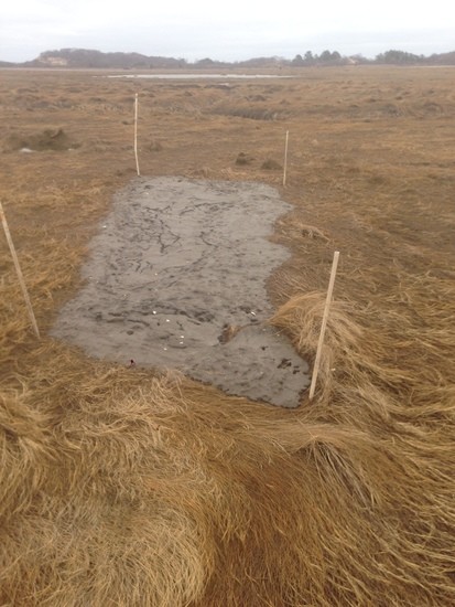
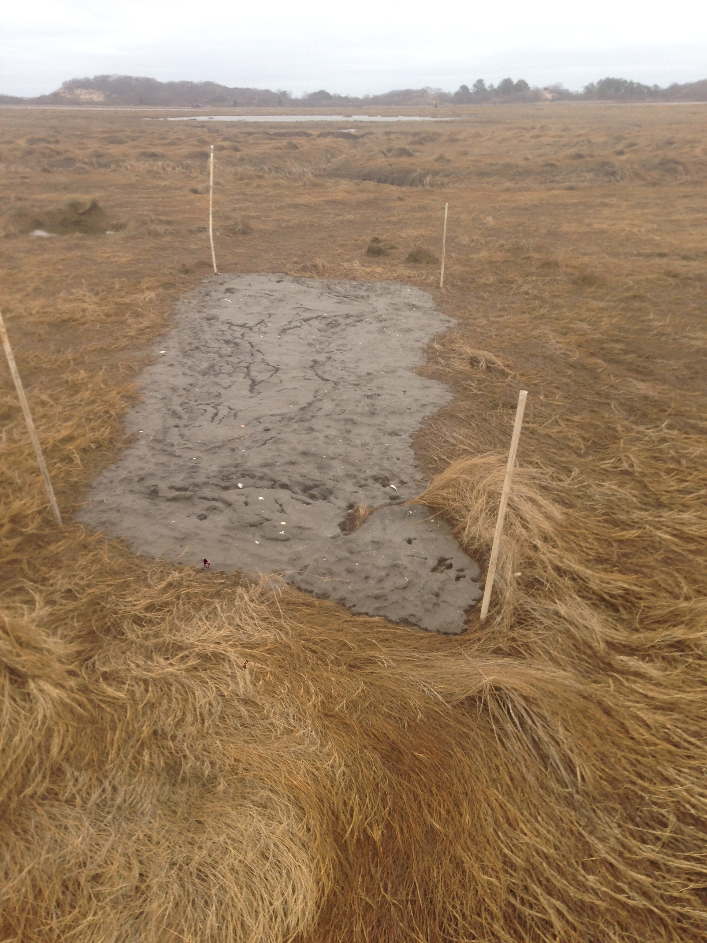
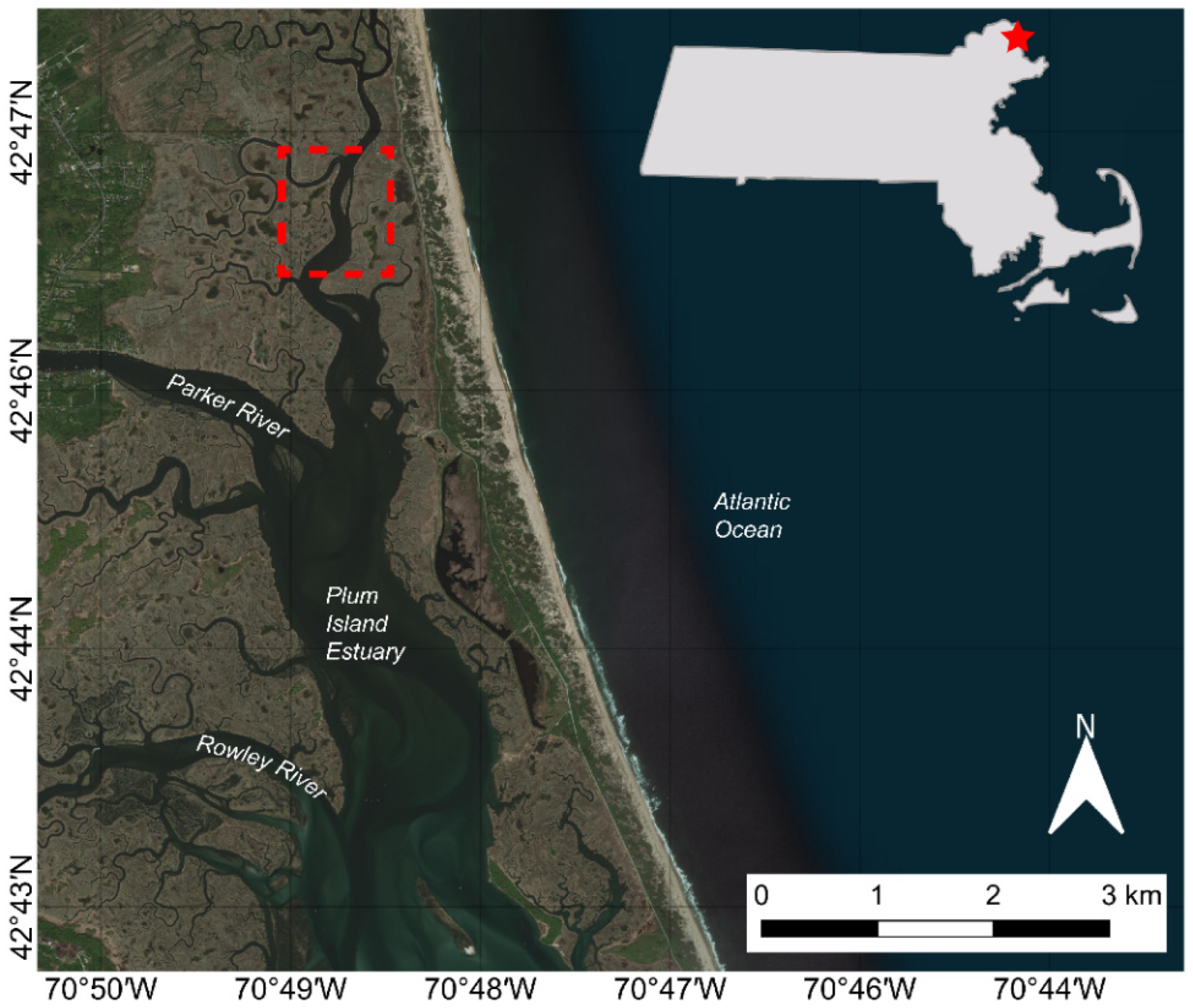
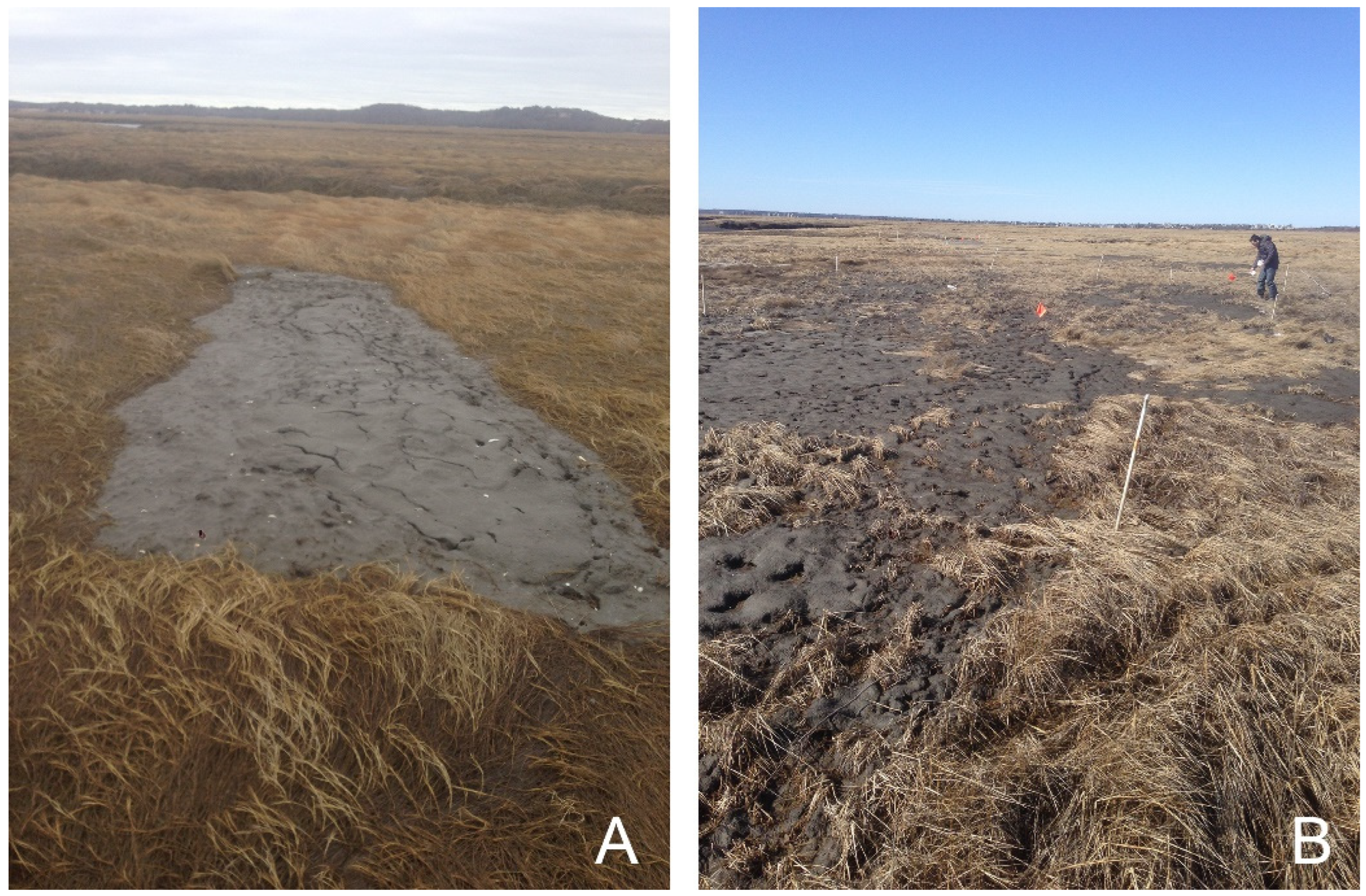
2.1. Site Description

Plum Island Estuary is an estuary-marsh complex in northeastern Massachusetts near the New Hampshire border. Our study site covers 1.45 km2 in the northern area of the PIE (Figure 1). Plum Island Estuary is connected to the Gulf of Maine through an inlet. The average mean tidal range at the NOAA buoy station 8441241, located offshore of Plum Island, is 2.8 m, and the mean tidal range within the estuary is 2.6 m [2,20]. The Ipswich, Parker, and Rowley Rivers debouch in the PIE sound. The Parker and Rowley Rivers drain a watershed of about 212 km2 [15]. PIE is composed of salt marshes, freshwater marshes, intertidal flats, and open-water tidal creeks and bays. Our study site is a salt marsh dissected by tidal creeks, and the marsh vegetation mainly consists of Spartina patens and Spartina alterniflora.
Water circulation in salt marshes involves the interaction between vegetation, topography, tides, and wind-driven currents [21,22]. Seasonal cycling influences the productivity of Spartina alterniflora and other marsh vegetation. Productivity rates of marsh vegetation peak during mid-summer, while mats of dead plant matter form during winter months [23]. Some previous studies suggest that marshes with higher tidal ranges, such as those in PIE, are more stable than marshes with lower tidal ranges with respect to sea level rise, because vegetation can survive in a larger range of elevations [7,24,25].
Salt marshes in PIE are subject to ice events during winter months. Ice disturbances, often associated with severe winter storms, move sediment from channels to the marsh platform through ice rafting and scouring [26]. Because ice tends to accumulate on tidal flats at low tide, tidal cycles influence the frequency and quantity of ice rafts. These ice rafts are responsible for the deposition of coarser sediment (e.g., silt and sand) on marsh platforms [10].
During winter storm Grayson on 4 January 2018, the water level reached a maximum of 2.93 m above NAVD88 at the Boston NOAA station (8443970), one of highest levels ever recorded. Maximum offshore wave heights reached 7.7 m [27]. Rafted ice from the storm resulted in the transport of large patches of sand and mud from tidal flats and the bottom of channels in PIE onto the marsh platform (Figure 2). These patches are identifiable in aerial imagery collected after the storm. This project uses aerial imagery collected before and after the storm to quantify the amount of IRD deposited during the event and interpret the importance of IRD to annual patterns of sedimentation in PIE.

2.2. Structure from Motion Photogrammetry

On 14 November 2017 and 27 February 2018, using a camera mounted on a 3DR Solo unmanned aircraft vehicle (UAV), true-color and 5-band multispectral imagery surveys were collected over 1.45 km2 of PIE. True-color imagery was collected using a Ricoh GRII digital camera and 5-band multispectral imagery was collected using a MicaSense RedEdge 3 camera. The images were collected at an altitude and with sufficient overlap to generate 2.5 mm resolution digital elevation models (DEM) using Structure-from-Motion (SfM) photogrammetry with Agisoft PhotoScan Professional software. Accuracy and precision were improved with 24 ground-controlled points on the marsh platform and a transect of 57 points on a nearby road. The points coordinates were measured with a high-precision Real Time Kinematic Global Position System [27]. After post-processing, the DEMs had a measured horizontal accuracy of 7 cm and 10 cm vertical accuracy. The accuracy was relatively low because of the complex vegetated surface. complete details of imagery and GCP acquisition can be found in [27,28]. The DEMs, orthophotos and multi-spectral imagery were referenced to the North American Datum of 1983. Complete details can be found in associated data releases.

2.3. Pixel-Based Classification

All classification and associated DEM and accuracy analysis were performed using ArcGIS 10.6.1 from the area of intersection between the 2017 and 2018 orthoimages. The classification method used a combination of pixel-based classification, elevation data, and accuracy assessment, which has been successfully used to detect marsh features in prior studies [29].
The 2017 orthoimage was classified using Iso Cluster unsupervised classification. All bands were used from the Ricoh true color imagery, and each pixel of size 2.5 mm was assigned to one of 26 classes. All clusters containing less than 20 pixels after the classification process were eliminated. The 26 classes were evaluated and combined into three categories that represented water, deposited sediment, and marsh vegetation.
Trained maximum likelihood classification (MLC) was the preferred method for the 2018 orthoimage because it minimized the number of misclassifications of IRD. For the 2018 imagery the true color bands were used. The training samples categorized water, sediment deposits, high-contrast marsh vegetation, low-contrast marsh vegetation, and shrub as separate classes. These categories were then evaluated and combined with marsh vegetation, water, and sediment.
The digital elevation model derived from SfM was used to separate intertidal channel sediments from sediments deposited on the marsh platform. The elevation data were reclassified into two categories representing areas above and below a specific water level. A value of 1.2 meters above mean sea level (NAVD88) was used as the breakpoint because it effectively separated ice-raft deposits on the marsh platform from the low-elevation sediment deposits in the tidal flats and close to the channels. The typical elevation of the salt marsh in Plum Island Sound is 1.4 m above NDV88, while the storm surge reached an elevation of 2.93 m at the NOAA station in Boston (8443970). The 1.2 m threshold, therefore, separates the marsh platform from tidal flats and channels also when the vertical error of 10 cm is accounted for. For both classified maps, areas with elevation below this threshold were re-categorized as water. Further processing was performed on the 2018 classification to convert it into a binary IRD/non-IRD output. First, the orthoimages and classified maps from 2018 and 2017 were compared to ensure that the classified 2018 sediment deposits included only IRD that were deposited during the storm. Then the water and the vegetated marsh platform categories were combined, and the final classification output defined each pixel as IRD or non-IRD.
Both automated and manual editing techniques were used with the classified maps to reduce the number of misclassifications. A combination of editing tools within the ESRI ArcMap 10.6.1 Spatial Analyst toolbox were used to merge clusters of under 100 pixels to the surrounding class. Manual editing was implemented where larger clusters of misclassified pixels were present. These clusters were corrected to the surrounding class based on comparisons with the ortho-imagery.

2.4. Accuracy Assessment

The classified maps were compared to a set of reference points to assess accuracy. The reference points were categorized based on whether IRD was visible in the ortho-imagery. Four hundred reference points were randomly created. Two hundred points were distributed within the area that did not contain IRD. The other two hundred points were distributed within the area that contained IRD. A confusion matrix was computed to assess general accuracy, user’s accuracy, and producer’s accuracy. General accuracy was calculated as a Kappa index of agreement, which measures overall agreement. U-accuracy shows false positives, or type 1 errors, and P-accuracy shows false negatives, or type 2 errors. U-accuracy for IRD assesses clusters that are incorrectly classified as IRD, and P-accuracy for IRD assesses the instances where areas containing IRD are not classified as IRD.

2.5. Field Survey and Sediment Analysis

The study area was visited on 9 April 2018, with the aim of collecting sediment samples and measuring IRD deposits. Twenty-six sediment samples were collected from 15 sediment patches in one portion of the study area. A wet sieving procedure was used to characterize the grain size of sediment deposits due to ice rafting. The procedure consisted of separating the fraction of fine materials (clay and silt) from the fraction of coarse material (sand and gravel). Approximately 50 cm3 of each sediment sample was first sonicated for 15 minutes at room temperature (~24 °C) in a beaker, filled with 100 cm3 of water, to separate aggregated particles. The material was then separated into sand and silt/clay fractions with a 63 µm sieve. Twenty-six undisturbed 5 cm3 volumes of sediment sample for each sediment patch were collected, dried at 60 °C, and weighed to determine sediment density. The sediment was then burnt in a furnace at 375 °C for 16 h. Once cooled down, fine sediment samples were weighed and the LOI (loss on ignition) was calculated. The thickness of the IRDs was finally measured in the field at 33 locations with a caliper. In Table 1 the percent of sand, sediment density, LOI, and deposit thickness are reported for each sample.

3. Results

3.1. Image Classification

Comparison of DEMs from 2017 and 2018 flights indicate only minor differences in elevation. In 2017, 88.5% of the study site had elevation values between 0 and 2 meters with respect to NAVD88. In 2018, 88.9% of the site fell within that range. The mean lower low water level (MLLW) for the domain’s tidal channel is −1.59 m (NOAA station 8441241). All elevation values below MLLW and above 4 meters were omitted (Figure 3). Changes in elevation caused by IRD were not detected due to the vertical accuracy of the DEM.
The 2017 map classified 54.2% of the total domain area as marsh, 40.4% as water, and 5.4% as sediment deposits (Figure 4). The 2018 map classified 73.7% of the domain as marsh, 24.8% as water, and 1.5% as sediment. The water-filled channels and ponds appear to cover a greater area in the 2017 imagery, probably because of the greater color contrast between wet-dry areas that was captured in 2017 (Figure 4a). In contrast, some of the ponds do not appear to be fully classified as water in the 2018 imagery. Pond extent depends on past rainfall and flooding events, and varies from month to month. Both images were taken at low tide, so tidal level was not responsible for differences in wet areas.
The final IRD-only classification map for 2018 indicates that the largest group of IRDs are deposited in three locations (Figure 5). The total domain area is 1.45 km2. The map identified 0.022 km2 of total IRD area within that domain. The IRD classified map (Figure 5) has an overall Kappa index of 0.92.

3.2. Field Survey

On 7 April 2018, field measurements recorded the location and thickness of 15 patches of IRD deposited after storm Grayson (Figure 2 and Figure 6). The area of each of the 15 patches was calculated based on its extent as measured from the classified map.
Figure 3. Digital elevation model of marsh surface derived with SfM. (A) shows elevation on 14 November 2017. (B) shows elevation of the same domain on 27 February 2018.
Remotesensing 14 05499 g003
Figure 4. True color orthoimages (A,B) and corresponding classified land cover maps showing water (dark gray), marsh (gray), and sediment (yellow). Tiles (A,C) show data from 14 November 2017; tiles (B,D) show data from 27 February 2018.
Remotesensing 14 05499 g004
Based on the 2018 field measurements (Table 1), the average thickness of IRD deposited at the study site after Grayson was 2.9 ± 0.69 cm. The thickness was relatively constant in each patch even along the patch borders, with a standard deviation around 0.7 cm (Table 1). The vertical error of the DEM and the presence of vegetation before the event did not allow the derivation of the IRD thickness from the DEM.

3.3. Estimation of Sediment Accumulation

The thickness measurements were used with the total IRD area as quantified by the classification method (21670 m2) to estimate sediment accumulation and density. Overall sediment accretion was calculated by finding Vt/Ad, where Vt is the average thickness multiplied by total IRD area, and Ad is the above-water region of the study site as defined by the classified map (1,087,629 m2). Using this approximation, the sediment accretion was estimated to be 0.57 ± 0.14 mm. The average density of the samples was 0.76 ± 0.17 g/cc, Therefore, the average mass input of sediments to the marsh surface was 0.44 ± 0.14 kg/m2.
Figure 5. Classification of the 2018 ortho-imagery. (AC) are the classified IRD deposits located in the three rectangular areas reported in the ortho-image.
Remotesensing 14 05499 g005
Alternative calculations were made to estimate sediment accretion and density based only on the patches with measured field data. To address which areas within the study site are most likely to be affected by the IRD, marsh units based on flow accumulation and drainage direction were used (see Figure 6). These units represent the watersheds of each tidal creek and were derived from the DEM [30]. Instead of averaging patch thickness to calculate sediment accretion and density, Vt was determined by summing the average thicknesses of every patch that occupied the same marsh unit. In cases where individual patches overlapped marsh unit boundaries, the marsh units were aggregated and treated as one larger, combined unit. Three marsh units contained overlapping patches and were treated as one 0.1477 km2 area, which was estimated to have a sediment accretion of 0.30 ± 0.06 mm with a deposited sediment mass of 0.31 ± 0.06 kg/m2. One additional marsh unit of 0.092 km2 contained patches of IRD. This area’s estimated sediment accretion rate was 0.0040 ± 0.00095 mm, and its deposited sediment mass was 0.0041 ± 0.0009 kg/m2.
Figure 6. IRD patches that were measured in the field and identified in the classified map. The red circles show the points at which thickness was measured. The dark grey patches were identified by the map but not measured. The light grey patches were identified by the map and measured. The grey lines show the boundaries of conceptual marsh units based on tidesheds in Plum Island [30]. Tiles C1, C2, and C3 show 4 patches that overlap at least one marsh unit boundary.
Remotesensing 14 05499 g006

4. Discussion

The above results demonstrate the ability of high-resolution UAV orthoimages and DEMs to detect and classify IRD deposits in salt marshes. Where further constrained/supported by field measurements, they enable quantification of IRD accretion rates. Nevertheless, there are some methodological limitations that must be considered.
While UAS is a valuable resource for obtaining high resolution aerial imagery and DEMs with more flexibility than LiDAR and satellite imagery, it is subject to some errors [31]. The GPS units that were attached to each UAS have theoretical accuracy of 10m vertically and 3m horizontally. Accuracy and precision were improved with the addition of ground-controlled points, but some uncertainty of about 7 cm horizontally and 10 cm vertically remains. Some areas may also exceed that uncertainty. SfM imagery requires that objects within the domain stay still during flights. Areas with moving objects and water are subject to higher degrees of inaccuracy [31]. In our case marsh vegetation can oscillate even at low wind conditions.
A DEM vertical error in the order of 10 cm is common in salt marshes even when high resolution UAV datasets are used. [32] obtained an elevation error of 5.9 cm with an UAV-Based LiDAR and 17.2 cm with UAV Digital Aerial Photogrammetry, [33] reported an error of 19.9 cm using UAV images. This error is caused by the dense and complex vegetation that shades the ground, preventing the precise calculation of the marsh platform elevation [34]. Depending on vegetation cover, it is often impossible to photograph the salt marsh ground even in winter months. This was the case at our field site, where a dense canopy of Spartina patens is always present (see areas around the sediment patch in Figure 2). This problem is also present in LiDAR data, with a difference or around 10–15 cm between the lowest elevation where the signal can penetrate the vegetation and the ground surface [35].
Ref. [36] reduced the vertical error of UAV-based Structure-from-Motion photogrammetry to 2.7 cm for elevation and 1.0–2.9 cm for horizontal displacement. However, they used large disks (30 cm) as UAV targets for the uncertainty estimate. The disks likely compressed the vegetation below them thus reducing the error. In normal conditions, with vegetation cover above the ground, the error is higher. [37] used UAV photogrammetry to map salt marsh channels. They obtain a vertical error of 5.7 cm, higher than the horizontal resolution of the images and DEM (3 cm) because of the offsets generated by aboveground plants. The error in channel width measurements was around 24 cm and caused by marsh vegetation shielding the banks. In unvegetated areas, like mudflats, DEMs can be obtained with higher accuracy (i.e., 2.2 cm horizontal and 2.7 cm vertical [38]).
Vegetation height and density vary seasonally, and therefore the comparison between DEMs taken months apart is also subject to error. An imagery-based land cover classification is therefore more suitable to identify IRD, and ancillary data surveyed in the field (i.e., deposit thickness and sediment density) can help assessing the volume and mass of the sediment delivered to the marsh during a storm.
Nevertheless, any generated land cover classification may also contain inconsistencies stemming from the original TCI/multispectral imagery. Some inaccuracies in the land-cover classification are associated with inconsistencies in the true color imagery. High-contrast shadows and light-quality differences between adjacent mosaicked orthoimages can lead to false classification. Some of the ponds detected in 2017 were not classified as ponds in 2018 (Figure 4D). This is likely due to differences in water level (Figure 4A,B). Salt marsh ponds are known to contract and expand as a function of flooding events and rainfall [39]. While high resolution imagery allows for the creation of detailed classification maps, it introduces problems when measuring errors. To get statistically significant measurements of accuracy, more and better distributed reference points would potentially be required [40,41]. In this project, the accuracy of classified IRD patches was measured more thoroughly than that of the surrounding non-IRD marsh area. While the Kappa index shows reliable accuracy and is based on a standard number of reference points, the values of 1 for marsh U-accuracy and IRD P-accuracy could be overestimated.
The sediment accretion and density calculations based on field measurement of distinctive marsh units are likely underestimates due to the limited measurements available. Within both marsh units used for the analysis, there were a considerable number of large unmeasured patches of IRD that were excluded from the analysis (Figure 6). The patch measurements are constrained to one of three major sites of IRD deposition (site C in Figure 5). Within that site, there are still many unmeasured patches. The limitation of this dataset constrains the accuracy of the overall estimates, and subsequently limits the assessment of IRD importance to sediment accretion. However, the field measurements offered additional confirmation that this image-based classification method accurately identifies the spatial distribution of IRD. Each measurement point used for these estimates was located within the classified IRD area. With more field data to accompany geospatial analysis of aerial imagery, it is possible that IRD deposits can be quantified with relatively high accuracy and efficiency. It is important to note that both the thickness of deposited sediments and the sediment density are relatively constant in the measured patches. We are therefore confident that the extrapolation of the measured data to the entire area is meaningful, with an acceptable error.
Vegetated marshes in the northeast typically accrete between 2 and 10 mm annually, though those rates can vary greatly [42]. In Spartina alterniflora and Spartina patens marshes in New England, recorded annual sediment accretion rates have been as low as 1–4 mm per year, and sites recorded in Bridgewater Bay ranged from 26–102 mm per year [42]. Studies of Plum Island Estuary sedimentation rates have also yielded mixed results. In marshes near the Rowley River, low-elevation marshes, subject to longer and more frequent periods of flooding, have higher accretion rates than high-elevation marshes [43]. Plum Island Sound marsh elevation had to increase at a rate of at least 2.8 mm per year since 1920 to maintain elevation relative to sea level rise at a mean bulk density of 272 ± 22 kg/m3 [6]. The high saltmarsh platform in Plum Island Estuary is accreting at about 2.5 mm/y [44], at about the same rate as regional sea level rise. Considering this estimate of annual accretion in PIE and our highest estimate of IRD-related sediment accretion at ~0.57 mm, ice-rafted sediment at this location accounts for over 20% of annual sediment accretion.
The prior estimate of the volume of sediment deposited by Grayson on the entire salt marsh was 18,000 m3, equivalent to a thickness of 0.6 mm, if spread evenly [19]. Our estimate in our high-resolution site is very similar (0.57 mm), confirming the validity of the estimate at different spatial scales and with different methodologies. The mineral fraction of our samples was also in the same range of the prior estimate [18], between 82 and 93% (see Table 1), suggesting that the measurements in this study are representative. The thickness of the ice-rafted deposits measured herein (2.9 ± 0.69 cm) is very close to the prior measurements, reporting a thickness of 3.19 cm [19], and another prior study [44], 3.01 ± 0.21 cm at different locations. We therefore conclude that the sediment layer entrained in the rafts is relatively constant in thickness. This thickness likely reflects the active, mobile sediment layer in the tidal flats, below which the sediment is more compacted with higher soil strength. It could also be a consequence of the high-degree of cohesion driven by Extracellular Polymeric Substances (EPS) that characterizes the first layer of tidal flat sediments [45,46].
Where ice-rafted deposition occurred, the 2.9 cm thickness represents ~12 years of normal deposition, as already indicated by prior estimates [19,44]. However, our analysis in marsh units indicate that this deposition is highly variable at the small scale, with some watersheds receiving large amounts while others receiving very limited sediment deposits. Such uneven deposition affects the geomorphology of the marsh platform and likely vegetation distribution. This analysis also assumes that conditions shortly after the IRD deposits were formed, caused by high tides and associated re-working of the deposits, did not induce significant changes.
A prior study [47] reported the stratigraphy of a sheltered salt marsh in Rhode Island, only 60 km from our study site. That study found and radiocarbon-dated tidal mud and low marsh deposits in the stratigraphic record of a high marsh. They interpreted this stratigraphy as widespread erosion caused by hurricanes, with subsequent filling with mud from tidal flats and recolonization by vegetation. Here we put forward the hypothesis that some of these deposits, particularly the thinner ones, could have been caused by ice rafts. If preserved in the stratigraphic record, the tidal mud layer deposited during Grayson would look similar to the subtidal deposit found by [47]. Deposition would also disturb the vegetation mat, favoring the recolonization with low marsh species. Some of these deposits would not indicate erosive events triggered by hurricanes, but rather deposition caused by ice rafts during high storm surges in winter.
Global warming could decrease the formation of IRDs, with warmer winters and less frequent freezing conditions. On the other hand, global warming increases sea level and therefore the frequency of extreme storm surges [48], which are the key mechanism for the transport of ice rafts on the marsh surface. High water levels are in fact necessary to move the largest rafts. It is therefore difficult to forecast the effect of global warming on IRD, and more research is needed in this direction.

5. Conclusions

Land cover classification of high resolution orthoimagery and DEMs generated using SfM from UAS-acquired aerial imagery are useful tools for identifying and quantifying the distribution of ice-rafted deposits caused by winter storms. This technique produces an orthoimage at a very high resolution (2.5mm) and the construction of a DEM with a 7- cm horizontal and 10-cm vertical accuracy. After the Grayson storm in January 2018, classification maps produced from the UAS DEMs and orthoimagery indicated that IRDs covered 21,670 m2 in a section of Plum Island marsh in Massachusetts. The classification had a relatively high degree of accuracy. These data in combination with field measurements were used to estimate sediment accretion and total mass of sediment deposited. The average measured thickness of the deposits was 2.9 ± 0.69 cm, which translates to an average accretion of 0.57 ± 0.14 mm for the entire area of study. The mass of the deposited material was 0.44 ± 0.14 kg/m2. These data agree with other studies that measured deposition during the same event for the entire marsh but at a lower spatial resolution. We therefore conclude that the technique presented herein is well suited for the mapping of both large and small ice-rafted deposits at very high resolution.

Author Contributions

Conceptualization, S.S. and S.F.; methodology, S.S., G.N.; software, S.S.; validation, S.S.; formal analysis, S.S. and G.N.; investigation, S.S. and G.N.; resources, S.F.; data curation, S.F.; writing—original draft preparation, all authors; writing—review and editing, all authors; visualization, S.S. and G.N.; supervision, S.F.; project administration, S.F.; funding acquisition, S.F. All authors have read and agreed to the published version of the manuscript.

Funding

This research was funded by the Woods Hole Oceanographic Institution Summer Student Fellowship Program and NSF awards 2224608 (PIE LTER) and 1832221 (VCR LTER).

Data Availability Statement

The aerial imagery from unmanned aerial systems (UAS) flights are available in the USGS database (see [29,30]).

Acknowledgments

We want to thank Neil Ganju and Zafer Defne at the USGS Woods Hole Coastal and Marine Science Center for mentoring S.S. during the Woods Hole Oceanographic Institution Summer Student Fellowship Program.

Conflicts of Interest

The authors declare no conflict of interest. The funders had no role in the design of the study; in the collection, analyses, or interpretation of data; in the writing of the manuscript, or in the decision to publish the results.

References

  1. Gedan, K.B.; Silliman, B.R.; Bertness, M.D. Centuries of Human-Driven Change in Salt Marsh Ecosystems. Annu. Rev. Mar. Sci. 2009, 1, 117–141. [Google Scholar] [CrossRef] [PubMed] [Green Version]
  2. Hopkinson, C.S.; Giblin, A.E.; Tucker, J.; Garritt, R.H. Benthic Metabolism and Nutrient Cycling along an Estuarine Salinity Gradient. Estuaries 2006, 22, 863. [Google Scholar] [CrossRef]
  3. Sweet, W.V.; Hamlington, B.D.; Kopp, R.E.; Weaver, C.P.; Barnard, P.L.; Bekaert, D.; Brooks, W.; Craghan, M.; Dusek, G.; Frederikse, T.; et al. Global and Regional Sea Level Rise Scenarios for the United States: Updated Mean Projections and Extreme Water Level Probabilities Along U.S. Coastlines; NOAA Technical Report NOS 01; National Oceanic and Atmospheric Administration, National Ocean Service: Silver Spring, MD, USA, 2022; 111p.
  4. Chen, X.; Zhang, X.; Church, J.A.; Watson, C.S.; King, M.A.; Monselesan, D.; Legresy, B.; Harig, C. The increasing rate of global mean sea-level rise during 1993–2014. Nat. Clim. Change 2017, 7, 492–495. [Google Scholar] [CrossRef]
  5. Sallenger, A.H.; Doran, K.S.; Howd, P.A. Hotspot of accelerated sea-level rise on the Atlantic coast of North America. Nat. Clim. Change 2012, 2, 884–888. [Google Scholar] [CrossRef] [Green Version]
  6. Hopkinson, C.S.; Morris, J.T.; Fagherazzi, S.; Wollheim, W.M.; Raymond, P.A. Lateral Marsh Edge Erosion as a Source of Sediments for Vertical Marsh Accretion. J. Geophys. Res. Biogeosci. 2018, 123, 2444–2465. [Google Scholar] [CrossRef]
  7. Talke, S.A.; Kemp, A.C.; Woodruff, J. Relative sea level, tides, and extreme water levels in Boston Harbor from 1825 to 2018. J. Geophys. Res. Oceans 2018, 123, 3895–3914. [Google Scholar] [CrossRef]
  8. Chmura, G.L. What do we need to assess the sustainability of the tidal salt marsh carbon sink? Ocean Coast. Manag. 2013, 83, 25–31. [Google Scholar] [CrossRef]
  9. Morris, J.T.; Sundareshwar, P.V.; Nietch, C.T.; Kjerfve, B. Responses of Coastal Wetlands to Rising Sea Level. Ecol. Soc. Am. 2009, 83, 2869–2877. [Google Scholar] [CrossRef]
  10. Ganju, N.K.; Kirwan, M.L.; Dickhudt, P.J.; Guntenspergen, G.R.; Cahoon, D.R.; Kroeger, K.D. Sediment transport-based metrics of wetland stability. Geophys. Res. Lett. 2015, 42, 7992–8000. [Google Scholar] [CrossRef] [Green Version]
  11. Redfield, A. Development of a New England Salt Marsh. Ecol. Monogr. 1972, 42, 201–237. [Google Scholar] [CrossRef]
  12. Tognin, D.; D’Alpaos, A.; Marani, M.; Carniello, L. Marsh resilience to sea-level rise reduced by storm-surge barriers in the Venice Lagoon. Nat. Geosci. 2021, 14, 906–911. [Google Scholar] [CrossRef]
  13. Zhu, Q.; Wiberg, P.L. The importance of storm surge for sediment delivery to microtidal marshes. J. Geophys. Res. Earth Surf. 2022, 127, e2022JF006612. [Google Scholar] [CrossRef]
  14. Tognin, D.; Finotello, A.; D’Alpaos, A.; Viero, D.P.; Pivato, M.; Mel, R.A.; Defina, A.; Bertuzzo, E.; Marani, M.; Carniello, L. Loss of geomorphic diversity in shallow tidal embayments promoted by storm-surge barriers. Sci. Adv. 2022, 8, 1–13. [Google Scholar] [CrossRef]
  15. Dionne, J.C. Schorre morphology on the south shore of the St. Lawrence Estuary. Am. J. Sci. 1968, 266, 380–388. [Google Scholar] [CrossRef]
  16. Mcowen, C.J.; Weatherdon, L.V.; Bochove, J.V.; Sullivan, E.; Blyth, S.; Zockler, C.; Stanwell-Smith, D.; Kingston, N.; Martin, C.S.; Spalding, M.; et al. A global map of saltmarshes. Biodivers Data J. 2017, 5, e11764. [Google Scholar] [CrossRef] [PubMed]
  17. Wood, M.E.; Kelley, J.T.; Belknap, D.F. Patterns of Sediment Accumulation in the Tidal Marshes of Maine. Estuaries 2006, 12, 237. [Google Scholar] [CrossRef]
  18. Argow, B.A.; Hughes, Z.J.; FitzGerald, D.M. Ice raft formation, sediment load, and theoretical potential for ice-rafted sediment influx on northern coastal wetlands. Cont. Shelf Res. 2011, 31, 1294–1305. [Google Scholar] [CrossRef]
  19. FitzGerald, D.M.; Hughes, Z.J.; Georgiou, I.Y.; Black, S.; Novak, A. Enhanced, climate-driven sedimentation on salt marshes. Geophys. Res. Lett. 2020, 47, e2019GL086737. [Google Scholar] [CrossRef]
  20. Buchsbaum, R.; Purinton, T.; Magnuson, B. (Eds.) The Marine Resources of the Parker River-Plum Island Sound Estuary: An Update after 30 Years; Massachusetts Office of Coastal Zone Management: Boston, MA, USA, 1998.
  21. Sullivan, J.C.; Torres, R.; Garrett, A.; Blanton, J.; Alexander, C.; Robinson, M.; Moore, T.; Amft, J.; Hayes, D. Complexity in salt marsh circulation for a semienclosed basin. J. Geophys. Res. F Earth Surf. 2015, 120, 1973–1989. [Google Scholar] [CrossRef]
  22. Geyer, W.R.; Signell, R.P. A Reassessment of the Role of Tidal Dispersion in Estuaries and Bays. Estuaries 2006, 15, 97. [Google Scholar] [CrossRef]
  23. Squiers, E.R.; Good, R.E. Seasonal Changes in the Productivity, Caloric Content, and Chemical Composition of a Population of Salt-Marsh Cord-Grass (Spartina alterniflora). Chesap. Sci. 2006, 15, 63. [Google Scholar] [CrossRef]
  24. Kirwan, M.L.; Guntenspergen, G.R.; D’Alpaos, A.; Morris, J.T.; Mudd, S.M. and Temmerman, S. Limits on the adaptability of coastal marshes to rising sea level. Geophys. Res. Lett. 2010, 37, L23401. [Google Scholar] [CrossRef] [Green Version]
  25. Kirwan, M.L.; Guntenspergen, G.R. Influence of tidal range on the stability of coastal marshland. J. Geophys. Res. Earth Surf. 2010, 115, F02009. [Google Scholar] [CrossRef]
  26. Ewanchuk, P.J.; Bertness, M.D. Recovery of a northern New England salt marsh plant community from winter icing. Oecologia 2003, 136, 616–626. [Google Scholar] [CrossRef]
  27. Ganju, N.K.; Brosnahan, S.M.; Sturdivant, E.J.; Pendleton, E.A.; Ackerman, S.D. Aerial Imagery from Unmanned Aerial Systems (UAS) Flights–Plum Island Estuary and Parker River NWR (PIEPR), February 27th, 2018; U.S. Geological Survey Data Release: Reston, VA, USA, 2019. [CrossRef]
  28. Cramer, J.C.; Brosnahan, S.M.; Ackerman, S.D.; Pendleton, E.A.; Sturdivant, E.J.; Borden, J. Aerial Imagery Collected during Unoccupied Aircraft Systems (UAS) Operations in Massachusetts and Maine between March 2018—September 2018; U.S. Geological Survey Data Release: Reston, VA, USA, 2021. [CrossRef]
  29. Farris, A.S.; Defne, Z.; Ganju, N.K. Identifying Salt Marsh Shorelines from Remotely Sensed Elevation Data and Imagery. Remote Sens. 2019, 11, 1795. [Google Scholar] [CrossRef] [Green Version]
  30. Defne, Z.; Ganju, N.K. Conceptual Marsh Units for Plum Island Estuary and Parker River Salt Marsh Complex, Massachusetts; U.S. Geological Survey Data Release: Reston, VA, USA, 2018. [CrossRef]
  31. Deliry, S.I.; Avdan, U. Accuracy of Unmanned Aerial Systems Photogrammetry and Structure from Motion in Surveying and Mapping: A Review. J. Indian Soc. Remote Sens. 2021, 49, 1997–2017. [Google Scholar] [CrossRef]
  32. Pinton, D.; Canestrelli, A.; Fantuzzi, L. A UAV-based dye-tracking technique to measure surface velocities over tidal channels and salt marshes. J. Mar. Sci. Eng. 2020, 8, 364. [Google Scholar] [CrossRef]
  33. Taddia, Y.; Pellegrinelli, A.; Corbau, C.; Franchi, G.; Staver, L.W.; Stevenson, J.C.; Nardin, W. High-resolution monitoring of tidal systems using UAV: A case study on Poplar Island, MD (USA). Remote Sens. 2021, 13, 1364. [Google Scholar] [CrossRef]
  34. Hladik, C.; Alber, M. Accuracy assessment and correction of a LIDAR-derived salt marsh digital elevation model. Remote Sens. Environ. 2012, 121, 224–235. [Google Scholar] [CrossRef]
  35. Rosso, P.H.; Ustin, S.L.; Hastings, A. Use of lidar to study changes associated with Spartina invasion in San Francisco Bay marshes. Remote Sens. Environ. 2006, 100, 295–306. [Google Scholar] [CrossRef]
  36. Kalacska, M.; Chmura, G.L.; Lucanus, O.; Bérubé, D.; Arroyo-Mora, J.P. Structure from motion will revolutionize analyses of tidal wetland landscapes. Remote Sens. Environ. 2017, 199, 14–24. [Google Scholar] [CrossRef]
  37. Chen, C.; Zhang, C.; Schwarz, C.; Tian, B.; Jiang, W.; Wu, W.; Garg, R.; Garg, P.; Aleksandr, C.; Mikhail, S.; et al. Mapping three-dimensional morphological characteristics of tidal salt-marsh channels using UAV structure-from-motion photogrammetry. Geomorphology 2022, 407, 108235. [Google Scholar] [CrossRef]
  38. Brunier, G.; Michaud, E.; Fleury, J.; Anthony, E.J.; Morvan, S.; Gardel, A. Assessing the relationship between macro-faunal burrowing activity and mudflat geomorphology from UAV-based Structure-from-Motion photogrammetry. Remote Sens. Environ. 2020, 241, 111717. [Google Scholar] [CrossRef]
  39. Wilson, C.A.; Hughes, Z.J.; FitzGerald, D.M.; Hopkinson, C.S.; Valentine, V.; Kolker, A.S. Saltmarsh pool and tidal creek morphodynamics: Dynamic equilibrium of northern latitude saltmarshes? Geomorphology 2014, 213, 99–115. [Google Scholar] [CrossRef]
  40. Congalton, R.G. A review of assessing the accuracy of classifications of remotely sensed data. Remote Sens. Environ. 1991, 37, 35–46. [Google Scholar] [CrossRef]
  41. Foody, G.M. Status of land cover classification accuracy assessment. Remote Sens. Environ. 2002, 80, 185–201. [Google Scholar] [CrossRef]
  42. Ranwell, D.S. Spartina Salt Marshes in Southern England: II. Rate and Seasonal Pattern of Sediment Accretion. J. Ecol. 2006, 52, 79. [Google Scholar] [CrossRef]
  43. Schmitt, C.; Wetson, N.; Hopkinson, C. Preliminary Evaluation of Sedimentation Rates and Species Distribution in Plum Island Estuary, Massachusetts. Biol. Bull. 1998, 195, 232–233. [Google Scholar] [CrossRef]
  44. Moore, G.E.; Burdick, D.M.; Routhier, M.R.; Novak, A.B.; Payne, A.R. Effects of a large-scale, natural sediment deposition event on plant cover in a Massachusetts salt marsh. PLoS ONE 2021, 16, e0245564. [Google Scholar] [CrossRef]
  45. Black, K.S.; Tolhurst, T.J.; Paterson, D.M.; Hagerthey, S.E. Working with natural cohesive sediments. J. Hydraul. Eng. 2002, 128, 2. [Google Scholar] [CrossRef]
  46. Fagherazzi, S.; Viggato, T.; Vieillard, A.M.; Mariotti, G.; Fulweiler, R.W. The effect of evaporation on the erodibility of mudflats in a mesotidal estuary. Estuar. Coast. Shelf Sci. 2017, 194, 118–127. [Google Scholar] [CrossRef]
  47. van de Plassche, O.; Erkens, G.; van Vliet, F.; Brandsma, J.; van der Borg, K.; de Jong, A.F. Salt-marsh erosion associated with hurricane landfall in southern New England in the fifteenth and seventeenth centuries. Geology 2006, 34, 829–832. [Google Scholar] [CrossRef]
  48. Lin, N.; Marsooli, R.; Colle, B.A. Storm surge return levels induced by mid-to-late-twenty-first-century extratropical cyclones in the Northeastern United States. Clim. Change 2019, 154, 143–158. [Google Scholar] [CrossRef]
Figure 1. Plum Island Estuary (PIE) in Massachusetts, USA; the boundaries of the study site are in red. ESRI image collected on 12 October 2021.
Remotesensing 14 05499 g001
Figure 2. (A,B) Examples of IRD sediment patches deposited by winter storm Grayson in Plum Island Estuary (PIE) in Massachusetts, USA, photos taken in April 2018.
Remotesensing 14 05499 g002
Table 1. Field measurements of 15 patches of deposited IRD within the study site. Thickness measurements were taken at multiple points within some large patches. Standard deviation is included for those averaged thickness values. Mean values of density, percentages of sand and organic matter for each patch are reported with their standard deviations.
Latitude, Longitude
(°)
Thickness (cm)IRD Patch Area (m2)Density (g/cc)% Sand% Mineral Sediment
42.7732098, −70.81165162.8 ± 0.6812.820.87 ± 0.1914.29 ± 2.8490.27 ± 2.28
42.7723858, −70.81324152.3 ± 0.78116.100.84 ± 0.0414.47 ± 2.3891.79 ± 2.03
42.7719599, −70.8130783.0 ± 0.61321.740.54 ± 0.137.77 ± 2.0785.95 ± 4.31
42.7727812, −70.81277173.2 ± 1.706.740.81 ± 0.1921.60 ± 1.0588.84 ± 1.93
42.7722308, −70.81319512.7 20.100.828.7781.39
42.7721826, −70.81311224.1 ± 0.60501.610.69 ± 0.2410.43 ± 1.6789.74 ± 3.02
42.7716978, −70.81334173.689.300.9723.5492.99
42.7721314, −70.81308363.9 ± 2.2382.380.534.6583.05
42.7721067, −70.81255653.015.860.8741.6292.11
42.7722182, −70.81250853.1 ± 0.5762.280.8911.4390.91
42.7725462, −70.81278652.75.23---
42.7727349, −70.81275292.812.990.8417.2990.71
42.7725084, −70.81220611.85.440.7622.4889.86
42.7725761, −70.8119692.08.220.8321.6189.07
42.7740023, −70.81173521.94.920.9919.0489.29
Publisher’s Note: MDPI stays neutral with regard to jurisdictional claims in published maps and institutional affiliations.

