1. Introduction
Climate warming has been observed for several decades, and polar regions serve as the best indicator of the rate of this phenomenon [
1]. The melting of glaciers in polar regions indicates that climate changes and the retreat of the ice cover are going to accelerate. Over recent years, the rate of glacier retreat has increased dramatically and, depending on the glacier type, it is from several to more than ten meters per day. Glaciers which terminate in the sea retreat towards the land faster than glaciers which do not terminate in the sea [
2,
3,
4]. This process is influenced by many factors, such as hydraulic characteristics of glaciers, their mass balance, temperature, humidity and wind speed [
5,
6]. The scale of glacier retreat depends on the velocity of ice flow from the glacial valley to the terminus [
4,
7]. In the case of tidewater glaciers, an increase in the ice flow velocity typically entails increased calving and retreat rates [
8]. An exception to the above fact is the glacier surge, which often leads to a significant glacial advance. In the case of such a phenomenon, the velocity temporarily increases and subsequently decreases.
For the above reasons, constant monitoring of glacier conditions is of great importance. However, their dynamics, size and often also location cause glaciers to be a difficult and demanding object of monitoring, especially in situ. Currently, the monitoring of glaciers is largely based on remote sensing techniques, including active synthetic aperture radar interferometry (SAR) systems.
SAR images are used inter alia to identify glacial zones on the basis of image classification [
9] and the shape of grounding lines in ice shelves [
10]. Glacier displacement velocities can also be estimated with the use of InSAR techniques [
11,
12]. However, the use of SAR differential interferometry in monitoring the velocity of glaciers may be of limited effectiveness due to decorrelations resulting from the velocity of ice mass movement [
13]. This effectiveness can be improved with the use of offset (feature)- and speckle-tracking techniques, which are based on SAR images (on the amplitude or on the amplitude and phase, respectively) [
14,
15].
Data regarding the displacement velocity of the ice cover have been provided in several research projects: globally in the MEaSUREs ITS_LIVE project [
13,
16], for Greenland [
17,
18,
19,
20] or for the Svalbard archipelago [
21]. The currently available data from the ITS_LIVE project are based on optical images from Landsat 4, 5, 7, 8 and are generalized to mean annual velocities. The data for Greenland are provided as part of the PROMICE project [
20] at approximately 12 day intervals, together with the acquisition of new images. The data provided by GFZ German Research Centre for Geosciences for Svalbard at monthly intervals are not updated regularly (they cover the period between January 2015 and November 2020). The above services provide data regarding only the displacement of glaciers, and do not include analyses of the results and/or of the relationships with the factors which induce such processes.
The aim of this research is to analyse the dynamics of a selection of nine glaciers terminating in Hornsund Bay in the Svalbard Archipelago region, between 2018 and 2022. Measurements of the movement of the ice masses velocities has been carried out using an offset-tracking technique based on Sentinel-1 SAR data. In contrast to the most of the projects and studies mentioned above, our work analyses ice flow velocity data defined over a 6- or 12-day time frame. This provides an opportunity to observe not only year trends, but also seasonal and instantaneous changes in ice flow velocity. The obtained results have also been analysed in the context of locally observed meteorological parameters.
2. Background and Methods
2.1. Study Area
Its location within the warm ocean currents causes Svalbard to be particularly prone to the influence of climate changes [
22]. According to Geyman et al. [
23] in the years 1936–2010 the surface of the Svalbard glaciers decreased by 10.4%, and their volume by 14.8%. Nuth et al. [
24] also indicate that the retreat rate of glaciers has increased after 1990. The flow velocities of the Svalbard glaciers are from several meters per year (in the case of land-terminating glaciers) to several hundred meters per year (in the case of glaciers terminating in tidewaters) [
3].
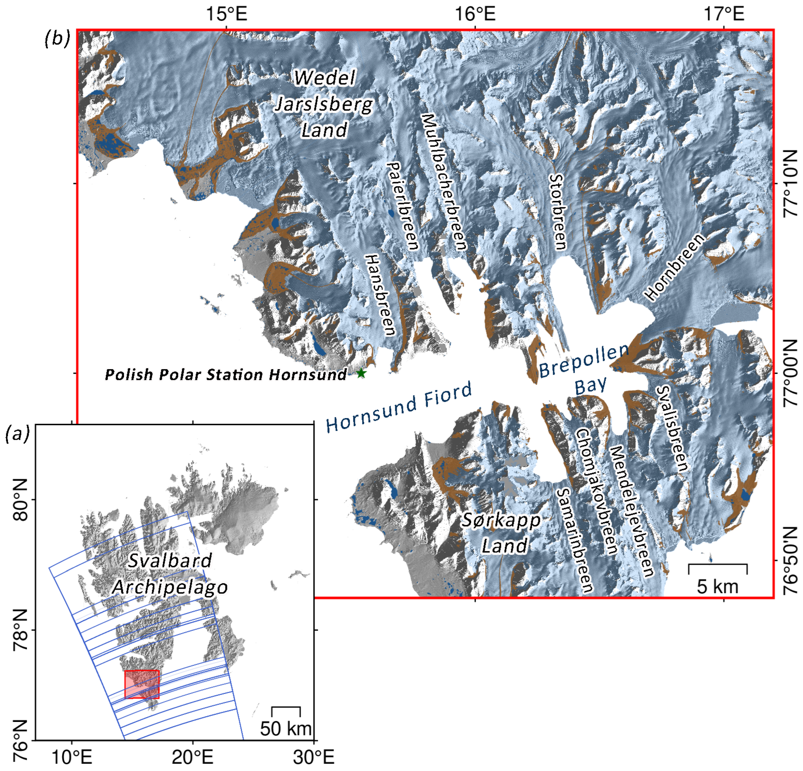
Hornsund is the southernmost fiord of the Svalbard Archipelago (
Figure 1). The glaciers of Hornsund are varied longitudinally. The ice cover increases from west to east. The mountain massifs furthest to the west are mostly free from ice, and mountain glaciers are situated between them. Further in the eastern direction, valley glaciers are present, and Spitsbergen-type glaciers are present only in the deepest part of the fiord [
25]. The majority of glaciers in the vicinity of Hornsund terminate directly in the fiord. This phenomenon results from the fact that their movement is due to basal sliding additionally accelerated by the presence of meltwater in the bed and by tidewaters at the terminus. In the case of some of the Hornsund glaciers, glacier surges were also observed, which consist in a temporal significant increase of glacier velocity, on occasions accompanied by the advance of the terminus [
25]. Since the end of the so-called Little Ice Age (LIA), i.e., since the beginning of the 20th century, the Svalbard glaciers systematically retreat [
26].
The retreat rate in Hornsund is one of the fastest in the entire archipelago, and in the 21st century, the ice loss accelerated to almost 2 km
per year [
4]. Since 1920, the retreating glaciers have been shaping the Brepollen gulf in the eastern part of the fiord. Its current surface is approximately 100 km
[
27].
The first velocity analyses based on the offset tracking technique for the Horsund region were presented for the 2012–2014 period by Błaszczyk et al. [
28]. The first regular measurements of glacier displacement velocities in Hornsund were enabled by the images from the Landsat 8 mission (provided as part of the ITS-LIVE program [
13,
16]). The annual data are available for 2014–2018. During this period, and especially in 2016–2018, most of the water-terminating Hornsund glaciers showed a tendency to increase their velocity accompanied by the retreat of their terminuses. The Paierlbreen was the most dynamic—in 2014 its velocity in the terminal area did not exceed 500 m/year [
16]. According to Błaszczyk et al. [
28], its mean velocity was 450 m/year, while in 2018, the velocities in the terminal area locally reached 1000 m/year.
Here, we present the results of our research for the years 2018–2021, for the nine biggest glaciers terminating directly in Hornsund. These glaciers, although all are valley in nature, are characterised by varying morphology, size and ice flow dynamics (
Table 1).
2.2. Data
We calculated the glacier flow velocities in the Hornsund region (
Figure 1) with the use of radar data from the Sentinel 1 satellite constellation. Unlike in the case of optical data (e.g., Landsat, Sentinel-2), radar data allow surface changes to be monitored in practically all weather conditions, regardless of the time of day or night. The images cover a period from January 2018 to the end of January 2022.
We used a total of 402 images from the ascending orbit No. 14 (
Table A1,
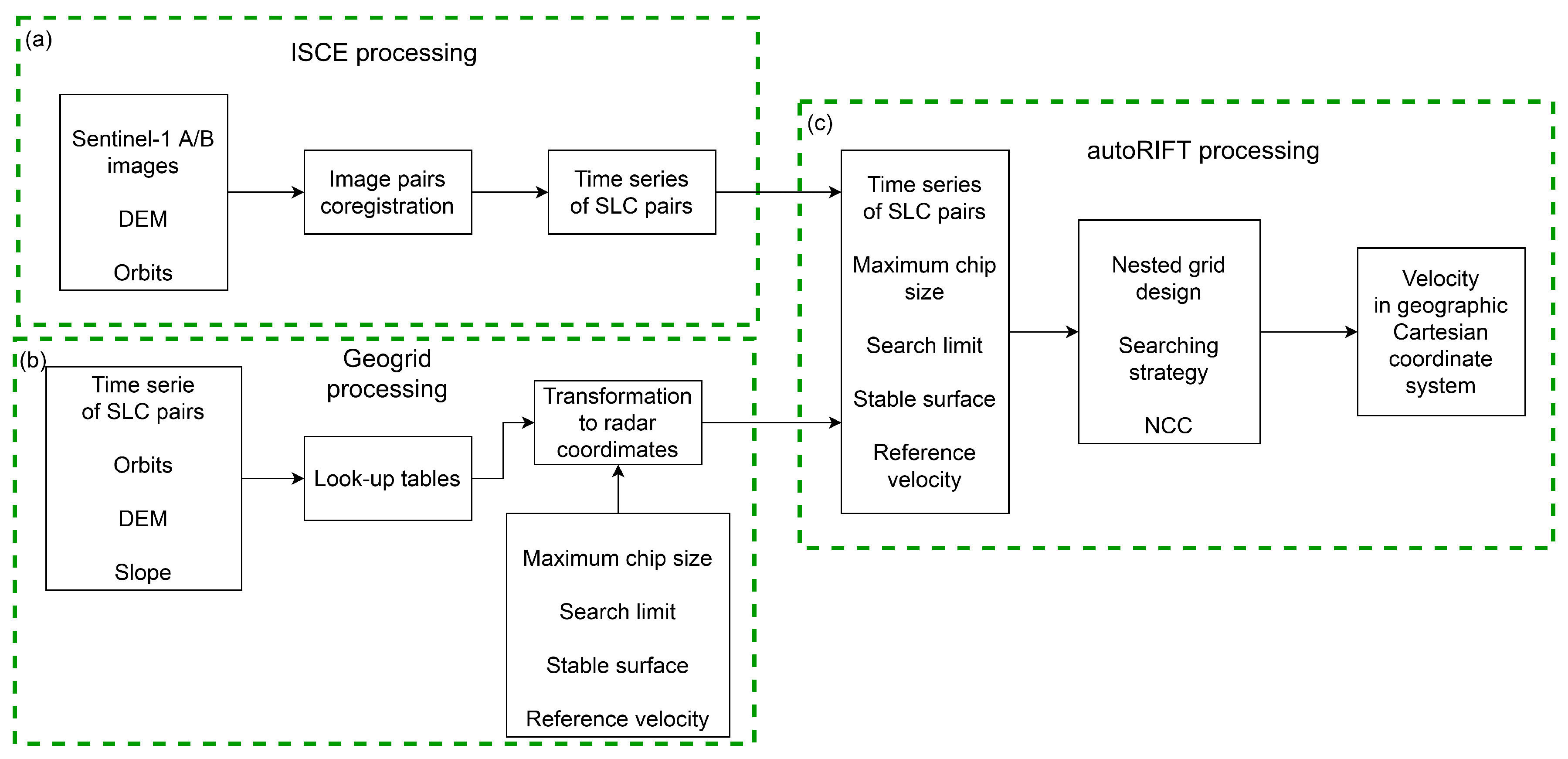
Appendix A). The preprocessing consisted of changing the raw Sentinel 1 Level 1.1 Interferometric Wide (IW) radar data into Single Look Complex (SLC). At this stage, image pairs were co-registered with an assumed six-day interval and time continuity. As a result of the above assumptions, a total of 236 interferograms were prepared. The set was a single continuous time series, in which the secondary image in the ith pair was simultaneously the reference image in the subsequent pair (i + 1). The period starting at the end of December 2021 was an exception, as the interval was increased to 12 days due to a failure of the Sentinel 1B satellite. The calculations were performed with the use of the ICSE software (
Figure 2a) [
29]. At this stage of our research, we used a high-resolution (32 × 32 m) numerical terrain model named ArcticDEM, which was developed on the basis of data from the constellations of Maxar optical image satellites [
30].
A permanent weather station is located in the vicinity of Polish research station in Hornsund, in the Isbjørnhamna bay (location: approx. 300 m from the northern shore of Hornsund, on an elevated sea terrace, approx. 10 m a.s.l.). However, the measurements at the station are performed locally, and are not representative of the entire, large area. Therefore, we analyzed the results with the use of C3S Arctic Regional Reanalysis (CARRA) weather data and of global sea surface temperature (SST) data, obtained from the Climate Data Store [
31] in the NetCDF format. The CARRA reanalysis system is based on the Numerical Weather Prediction system HARMONIE-AROME. Input data include the orography and physiographic database, lateral boundary (ERA5 4DVAR hourly analyses), synoptic and other surface observation, satellite data (snow cover, sea surface temperature, sea ice concentration) and upper air observations. The CARRA contains 3-hourly analyses and hourly short-term forecasts of atmospheric and surface meteorological variables. The horizontal resolution of the CARRA data was 2.5 × 2.5 km. Data regarding air and sea temperature, precipitation and wind speed were collected for each day at 12:00 (UTC). The temperature was identified for a point located 2 m a.s.l. in front of the glacier terminus. We believe that such a location allows a rational comparison of changing weather parameters (temperature, humidity, precipitation). Wind direction and velocity were identified for the same point, but at an altitude of 10 m a.s.l. in order to best reflect the changeable character of this value in polar conditions. Wind parameters are presented in the form of the wind rose for annual time intervals. Our analysis also allowed for the sea temperature in the vicinity of ocean-terminating glaciers. SST values were identified for points in front of the glacier.
Moreover, in order to present the fluctuation of weather parameters in Hornsund in a broader context, we used data from the permanent weather station located in the vicinity of Polish Polar Station, Hornsund. The data included average annual temperature, annual precipitation, average wind speed and sum total of sunshine hours for years 2014–2021 [
32].
2.3. Geogrid and AutoRIFT Inputs and Data Processing
We determined glacier displacement velocities in the area of Hornsund with the use of the Geogrid and autoRIFT environments [
16,
33]. The ice flow velocity is calculated with the use of autoRIFT, on the basis of the feature tracking technique. The technique uses SAR images and was borrowed from feature tracking algorithms for optical images, where it was already used at the beginning of the 1990s [
34]. In the investigated area, two images were compared in order to identify common (identical) features. This comparison was performed with the Normalized Cross-Correlation (NCC) algorithm. The algorithm searches for the maximum values of correlations between images allowing the identification of identical features. Subsequently, the values of their respective displacements (offsets) were calculated in the plane of both the slant-range and the azimuth (in the SAR image system) [
14]. In this approach, the Geogrid module is responsible for geocoding.
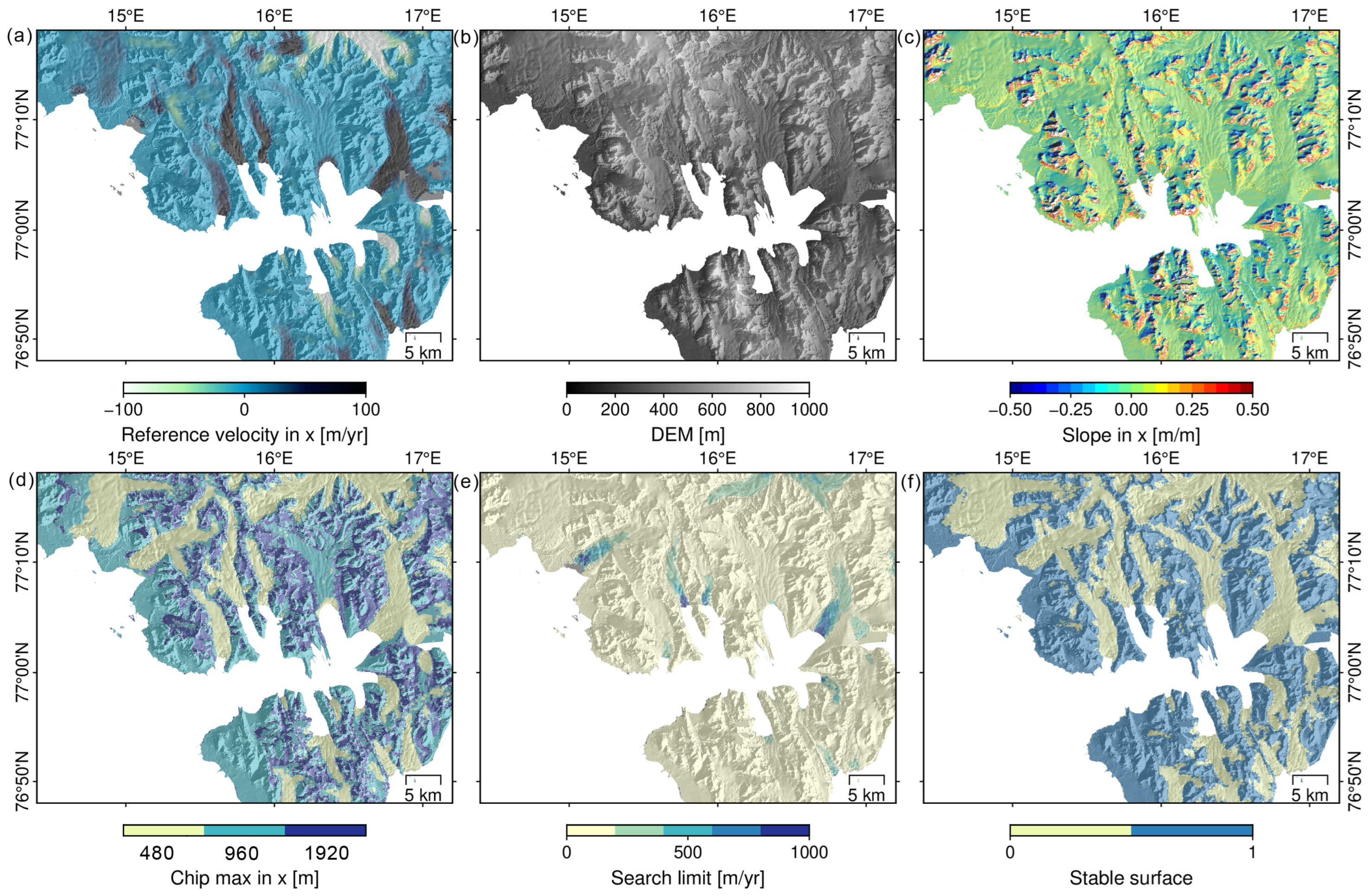
Apart from the preprocessed SAR data, the Geogrid and autoRIFT environments require additional input data (
Table 2 and
Figure 3). The numerical terrain model and its derivative—the slope model—was used in Geogrid (
Figure 2b), which allows the tracking of changes in the coordinates of SAR images on a geographic grid. For this purpose, two look-up tables were developed, which provide correspondence of individual points between two grids (pixels and coordinates) [
33]. In effect, the autoRIFT module (
Figure 2c) identifies displacements on the original coordinates of the image, and the result was introduced directly on the grid in the geographic Cartesian coordinate system (in our case it is EPSG:3413). All the input data were transformed and trimmed by the Geogrid module to match the coordinate grid and the SAR image range. However, the data were not resampled.
Table 2.
Input data description.
Table 2.
Input data description.
| Input | Description | Units | Coordinates |
|---|
| SAR image pair | Coregistered reference and secondary Sentinel 1 SAR images. The coregistration process is performed in the ISCE environment. Detailed description above. | local: range/azimuth | image |
| DEM (Figure 3b) | Digital elevation model with resolution 120 × 120 m above WGS84 ellipsoid. Resampled data from 32 m ArticDEM [30]. | m | EPSG:3413 |
| Slope (Figure 3c) | For data in map projected coordinate system. Rate of change in X and Y directions. Based on DEM data. | m/m | EPSG:3413 |
| Reference velocity (Figure 3a) | Reference mean ice velocity (2013–2017) based on ITS-LIVE Landsat ice velocity product. Separately for X and Y direction. Data from ITS-LIVE project [16]. | m/year | EPSG:3413 |
| Search limit (Figure 3e) | Range to search for displacement, based on reference velocity and proximity to the ocean (from topographic basemap datasets from Norwegian Polar Institute [35]). Separately for X and Y direction. | m/year | EPSG:3413 |
| Chip size (Figure 3d) | Maximum size of the chip (template) for correlation determination. Smaller chip size is lower accuracy with better resolution and bigger chip size is better accuracy with lower resolution. Own study for the Hornsund fjord area based on topographical basemap datasets from Norwegian Polar Institute [35]. | m | EPSG:3413 |
| Stable surface (Figure 3f) | Is defined by ice free areas (e.g., rocks) and stable ice caps. Own study for the Hornsund fjord area based on reference velocity and topographical basemap datasets from Norwegian Polar Institute [35]. | binary | EPSG:3413 |
The autoRIFT module searched for displacements using a nested grid, a combination of sparse and dense search, and a disparity filtering technique (as described in Lei et al. [
33]). In order to obtain a result of the highest possible resolution and accuracy, the chip size was individually adjusted each time [
13,
33]. The smaller the chip, the higher the spatial resolution, but at a lower accuracy. An increased chip size results in a lower resolution, but ensures a higher accuracy. The maximum and/or the minimum size of the chip should be decided a priori on the basis of the reference ice velocity values and reference terrain coverage (ice, rock, water). After the chip size was adjusted, a sparse search was performed in order to exclude low coherence areas, and this was followed by the proper dense search. The normalized cross-correlation was executed with the downstream search routine, which allowed the search limit to be reduced and which was possible owing to the a priori information on the reference velocity. In addition, the search limit was defined in the form of input data. The lower its value, the lower the expected image displacements.
As a result of using the Geogrid and autoRIFT algorithms, we obtained a time series of glacier displacement velocities in Hornsund for 4 full years, at 6-day average intervals.
2.4. Deviation Analysis
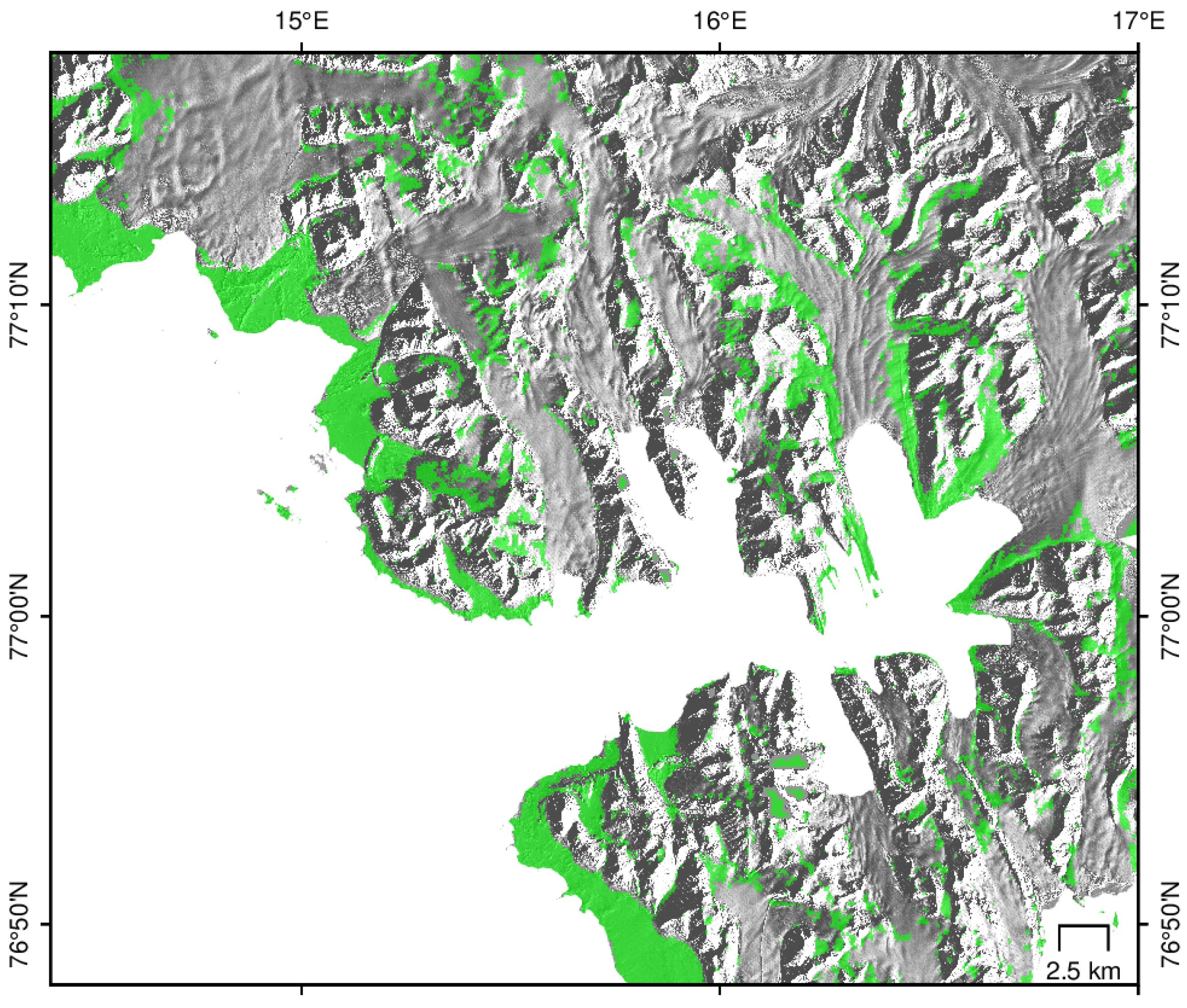
Assessment of the actual accuracy of glacier flow velocity determinations requires independent and convergently acquired reference data of high accuracy. In contrast to, e.g., the Greenlandic areas in the Svalbard archipelago, no other sources of reference data (e.g., high-resolution data from the TerraSAR-X satellite) are available for the area and period under study.
We identified the accuracy of our results by following an approach used by Lei et al. [
13], who determined the median absolute deviation (MAD) of the differences of obtained displacement velocity values from the reference value for areas identified as stable. In our case, the areas not covered with ice served as reference areas. Additionally, due to varied terrain relief, we marked out the areas with a slope greater than 5 degrees and we used the shape of the shoreline current as of 27 September 2021, developed on the basis of the Sentinel-2 image. The final reference area is shown in
Figure 4. We assumed the data presented in
Table 2 as the reference velocity value (
). Residual values (
) were determined according to the following Formula (
1).
The calculations were obtained for each SAR image pair (
i) and pixel (
n) in the reference area, where
were calculated velocities. Then, the MAD values for each pair were obtained (
) (
2).
The MAD value was defined collectively for the displacement vector. However, the geometry of SAR imaging causes the azimuth component (for the satellite coordinates) and the corresponding Y component (for the cartographic coordinates) to be more biased.
This approach is in line with previous work [
33], as well as the recommendations suggested by Paul et al. [
36] (recommended strategy: level-2).
3. Results
3.1. Variability of Ice Surface Velocity
Glacier velocity values in the Hornsund area vary even for glaciers that are close to each other. This difference is due to a combination of factors which may be attributed to individual glaciers.
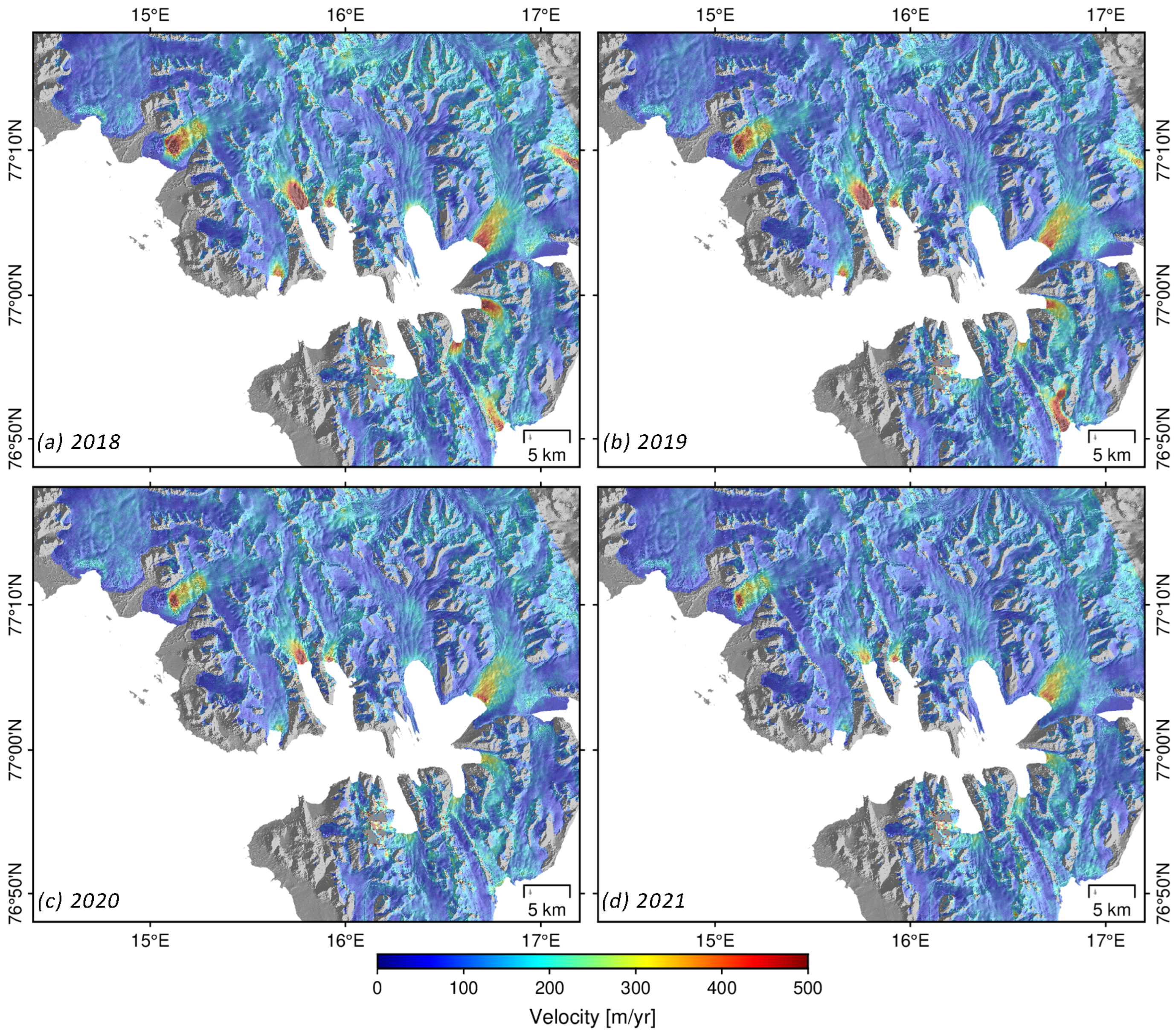
Figure 5 shows the changing velocities of the ice cover in the years 2018–2022. The highest velocities are observed on the Paierlbreen—they are approx. 700 m per year in 2018, and the lowest velocities are observed on the Storbreen—below 100 m per year (over the whole period analysed).
The results in the first place demonstrate that, since 2018, mean velocities of the ice cover in Hornsund decreased year to year (
Figure 5). This phenomenon is particularly visible in the case of two glaciers located in the northern fiord coast: Paierlbreen and Muhlbachenbreen, in which the velocity decreased most significantly in 2020 relative to the previous years. Decreased ice flow velocities were also observed in the case of the Hansbreen, Svalisbreen and Mendelejevbreen glaciers. The most limited differences in year-to-year ice flow velocities were observed on Storbreen, Hornbreen, Chomjakovbreen and Samarinbreen. However, in this group only Hornbreen reaches velocities exceeding 400 m/year in the area of its terminus.
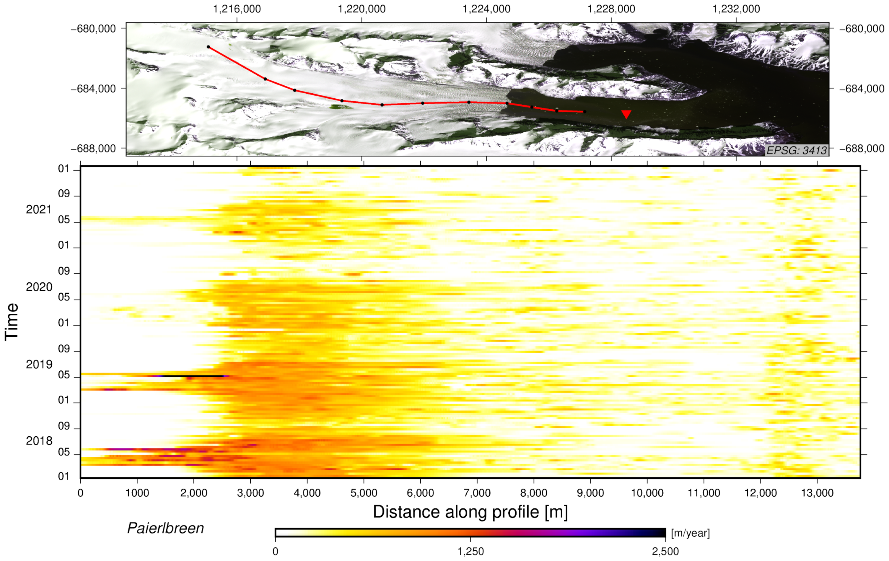
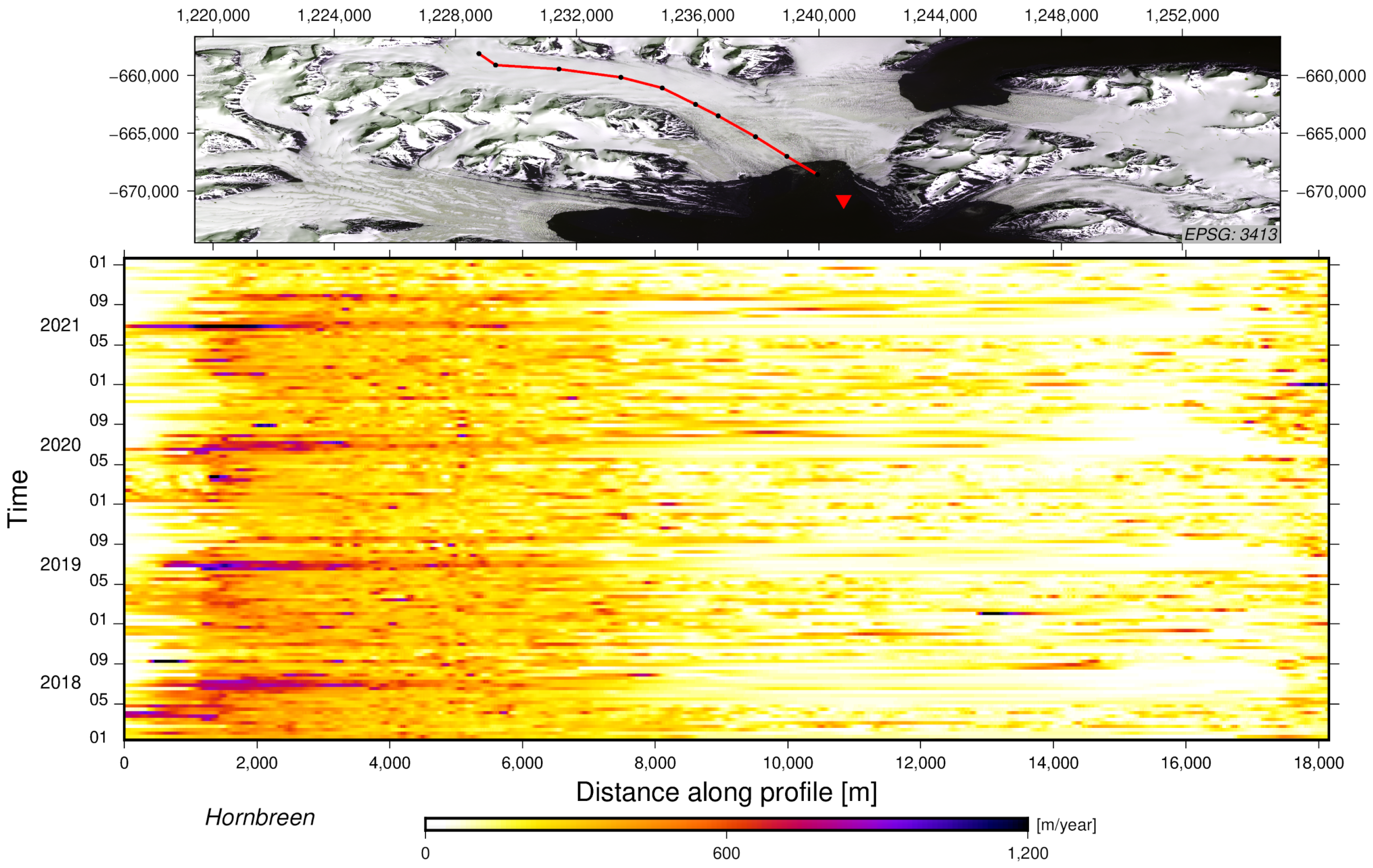
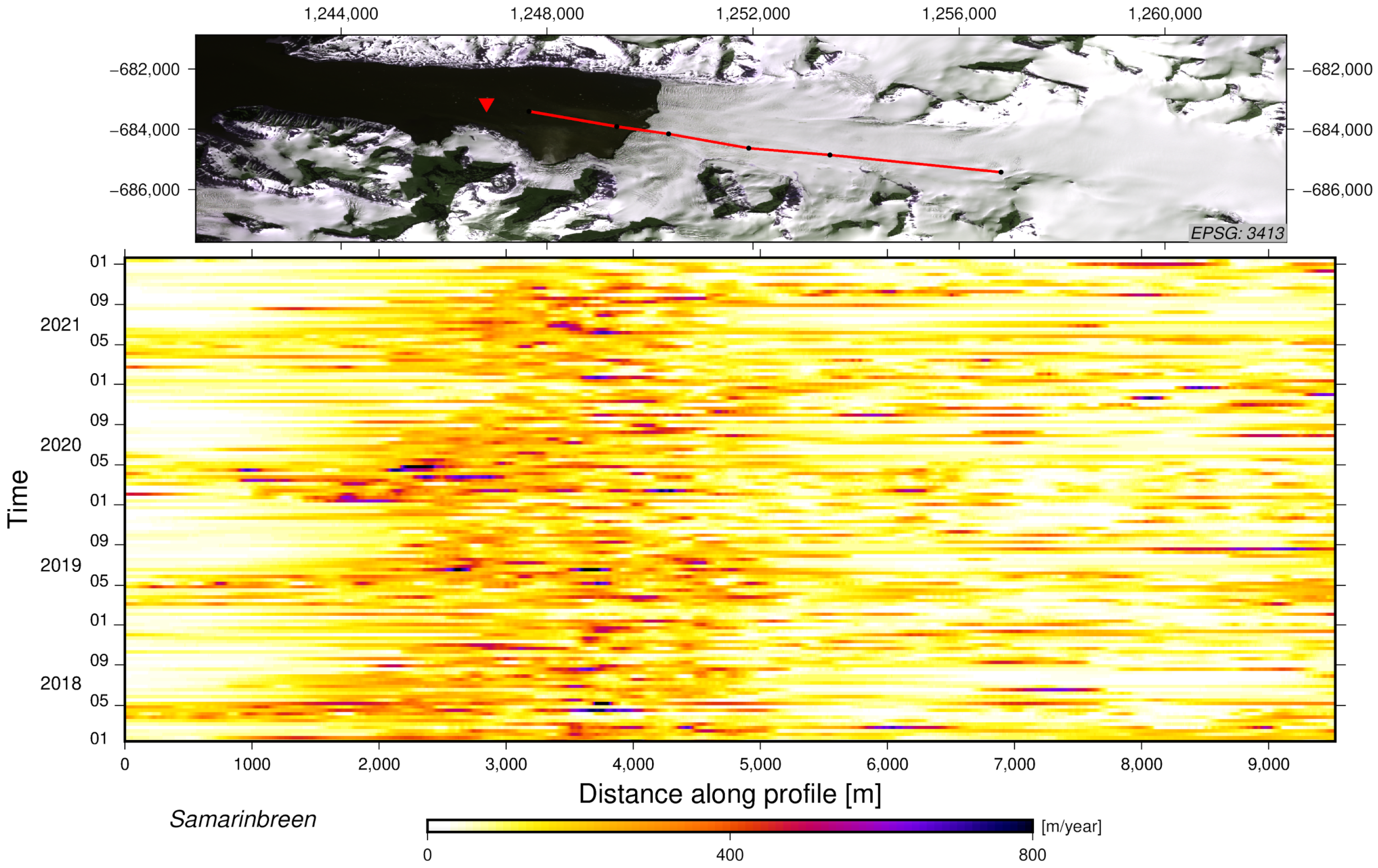
The results, presented as a consistent four-year time series with a short, six-day interval, allowed investigations of the glacier dynamics and its variability in time and space. Along each glacier, we defined lines for which we developed profiles from 5.5 to 18 km in length. They served to show the velocity values in time. In this article, we present profiles for Paierlbreen, Hornbreen and Samrinbreen (
Figure 6,
Figure 7 and
Figure 8). Profiles of velocity changes for the remaining glaciers addressed in this study are presented in the appendix
Figure A1,
Figure A2,
Figure A3,
Figure A4,
Figure A5 and
Figure A6.
Velocity distributions on the profile defined along Paierlbreen clearly indicate a velocity decrease during the analyzed four-year period. In the first two years (2018–2019), in the terminal area and most probably also in front of the terminus (0–2000 m of the profile), areas of high flow velocities were observed in the summer period. As they almost completely disappeared in the winter period, they may be attributed to the intensive calving process of the glacier. In the frontal area of Paierlbreen (2000–6000 m of the profile), the velocity changes also have a clearly seasonal character—the velocities decrease at the end of every ablation period (around September). The velocities clearly decrease in the further part of the profile and remain on a similar level for the entire observation period. Local velocity increases are observed in two areas (approx. 8500 m and between 12,000 and 13,000 m). They also remain similar for the entire observation period. We believe that this state is partly due to the topography of the glacier (its slope) and to the transitions between the ablation zone and the accumulation zone. Despite the velocity decrease during the four analyzed years, the glacier shows high dynamics caused by a relatively high slope, exposure to the south and being located in a narrow valley (see
Table 1). The twin glacier, Muhlbachenbreen, also shows high ice flow dynamics (see the
Appendix A,
Figure A4).
The Hornbreen has significantly lower dynamics than the Paierlbreen. However, it does not show a significant velocity decrease in the years 2020–2021. The seasonal character of the changes, and especially the decrease of velocity directly after the ablation period (September–January), can also be observed in this case. An interesting phenomenon occurs here: an annual increase of the spatial range (towards the center of the glacier) of the area showing higher ice flow velocities—from approx. 3000 m to 6000 m. As in the case of Paierlbreen, a local increase in ice velocity is observed throughout the year in the distal part of the Hornbreen profile.
Samarinbreen shows more variable dynamics of ice flow velocities than the above-discussed glaciers. It is located in the southern part of the fiord, retreated towards the land by approx. 8.5 km, and surrounded by high mountain peaks (up to 1433 m a.s.l.) in a glacial valley of a width increasing between the peaks. In this case, the dynamics of changes is also related to the seasons, albeit with significantly smaller differences observed. This fact is most probably due to the location of the glacier and to the limited influence of weather factors. A limited velocity decrease can be observed at the end of the ablation period (September–December). The most significant changes, reaching 2 m/day, are repeatable and can be observed between April and May in the front part of the glacier (2000–4000 m of the profile). Further along the profile, the dynamics clearly decreases (the highest values reach 1 m/day). More significant changes occur sporadically towards the end of the profile (up to 1.8 m/day). Over the four-year period, the glacier steadily flew into the sea. The rate of changes is similar in subsequent repeatable periods. In the summer, the dynamics is higher due to the flow of a part of the ice from the valley and to the calving of the glacier.
3.2. Seasonal Variations in Ice Velocity
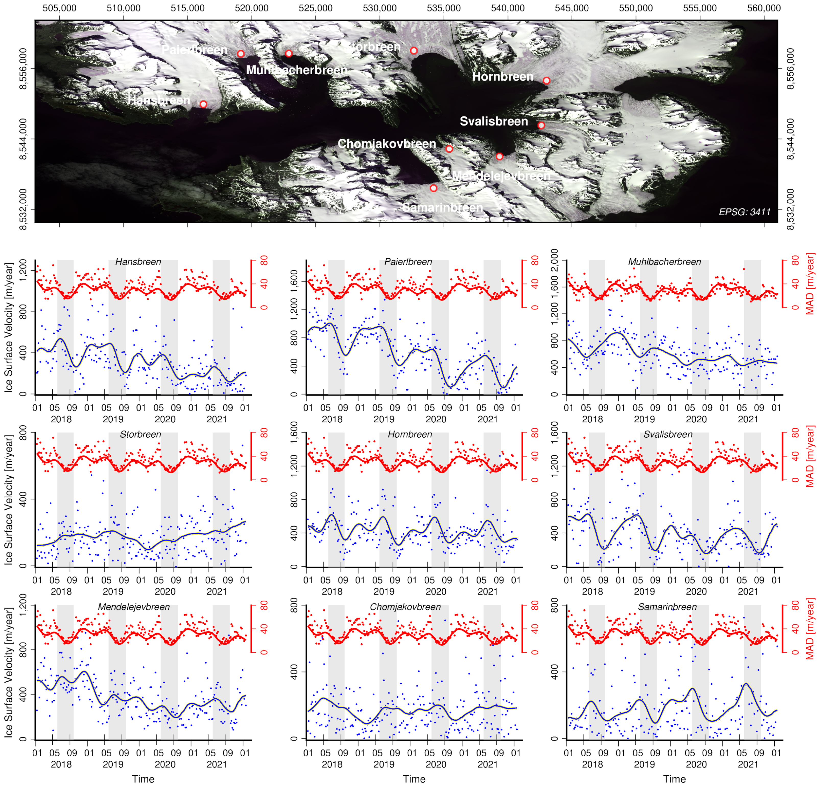
Additionally, for more detailed analysis, we precisely plotted the velocity changes for points selected on the most dynamic areas at the terminuses of the investigated glaciers (
Figure 9). We compared the velocities with the MAD values for the stable areas. For both variables (velocity and MAD), trend lines were determined based on time-consistent B-splines [
37].
The calculated MAD values for the summer period are significantly smaller in relation to the winter period (
Figure 9). This confirms that SAR data are sensitive to snow and ice conditions on the glacier surface. Observed during winter periods (October–May), maximum MAD values oscillate between 60 and 70 m/year. In contrast, during summer (June–September), MAD values range from 15 to 40 m/year. During the transitional periods between summer and winter, their values reach a maximum, which is related to the presence of water on the surface that has a significant impact on the accuracy of the offset tracking method based on SAR imagery [
36]. Analysis of the trends of the MAD values and ice mass velocities of the individual glaciers did not reveal a correlation between them. Seasonal increases or decreases in glacier velocity do not correlate with changes in MAD values. The amplitudes of the annual MAD values are much smaller compared to the amplitudes of ice mass flow velocities (for glaciers characterized by seasonality).
A clear, systematic velocity decrease is observed especially in the case of Paierlbreen. This fact serves as a confirmation of the above analysis results (
Figure 6 and
Figure 9). In the case of points located in the areas of Hornbreen, Paierlbreen, Samarinbreen and Svalisbreen, the long term trend indicated the seasonal character of the changes, during the entire four-year period (
Figure 9). The graphs show precisely that the velocities increase in the summer (June–August) and then decrease significantly around September and October. Between 2018 and 2019, the phenomenon is also observed in the case of the point located in the area of Hansbreen.
Our results (
Figure 5,
Figure 6,
Figure 7,
Figure 8 and
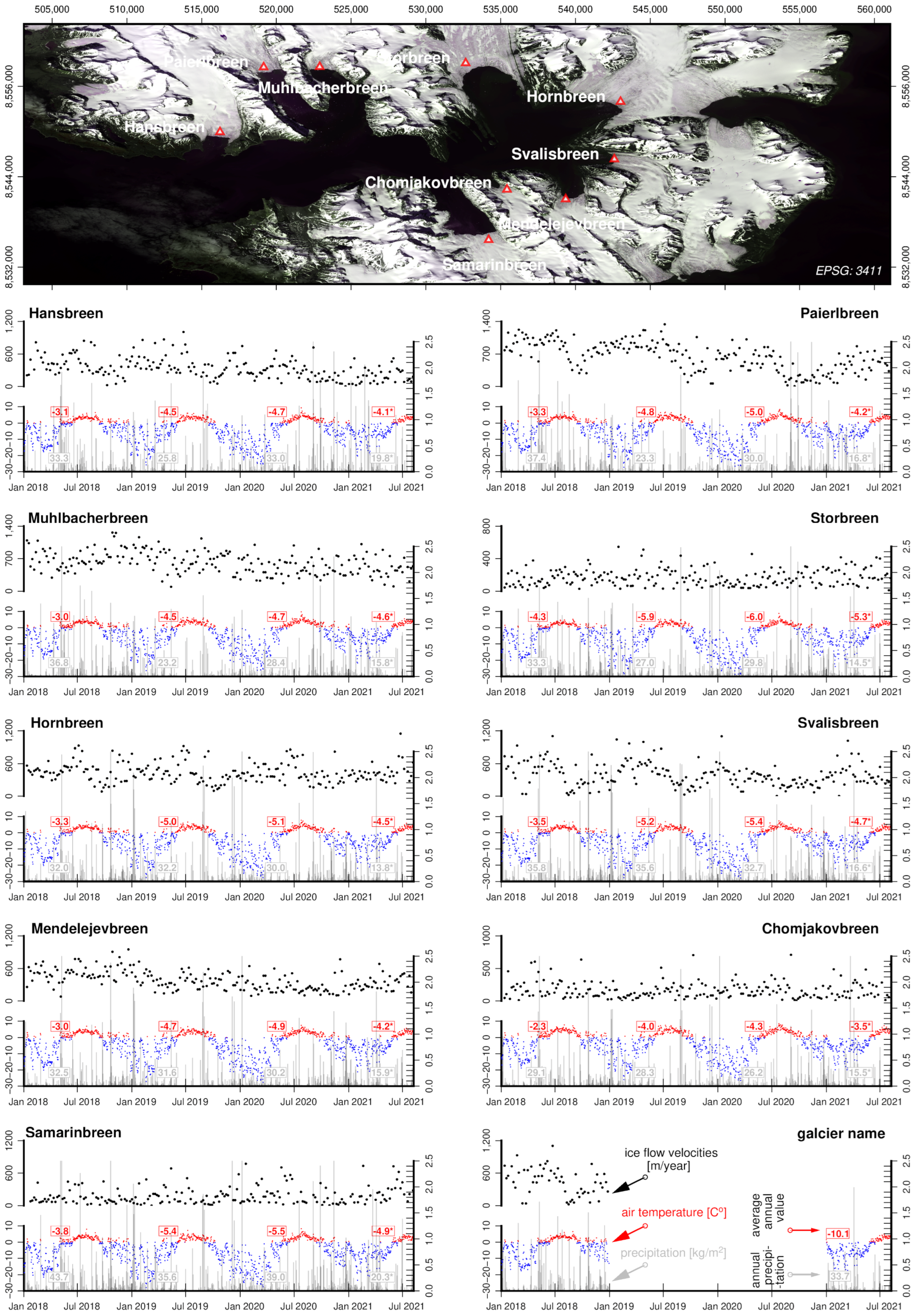
Figure 9) demonstrate that the year-to-year variability of ice flow velocities is a natural phenomenon and occurs every year. However, the dynamics of the glaciers shows also another variability, which is not linked to seasons and which is manifested in a velocity decrease after 2019 (except for Storbreen, which showed a slight upward trend). We further investigated this phenomenon by comparing weather data for the points located in the area of the analyzed glaciers (
Figure 10).
The data indicate that the year 2018 was exceptionally warm—in comparison to 2017, the average annual temperature increased by 0.23 °C, and in the subsequent years the temperatures decreased by more than 1 °C (
Figure 10 and data from [
32]). Between 2018 and 2019, the temperatures were higher than in the other years for all glaciers. Increased precipitation in the winter season (especially near Hansbreen and Paierlbreen between 2020 and 2021—see
Figure 10), in combination with low temperature, reduced the influx of water into the glacier—as a result—the velocity of ice surface movement to decrease in 2021 (see
Figure 6 and
Figure 9 for Paierlbreen and
Figure 9 for Hansbreen). Another reason for the different velocities of glacier surfaces may lie in the humidity and the level of atmospheric precipitation; 2019 was a particularly dry year in comparison to other years (the difference was almost 3-fold). The precipitation was very limited especially in the summer months.
The time series of the velocity values for all the investigated glaciers show peaks—single increases of velocities. On Chomjakovbreen, the peaks occur mainly towards the end of the ablation period, while on Svalisbreen they occur at the beginning of this period. Based on the analysis of the data shown in
Figure 10, we conclude no correlation between peak occurrence and increased precipitation and/or significant changes in air temperature (especially changes from negative to positive values). There is also no correlation between peak occurrence and increased MAD values.
4. Discussion
The results of our SAR data-based analysis in the Hornsund region allow the ice flow dynamics to be identified for the last four years. The dynamics of glacier flow velocity remains constant for the area of the entire fiord. Some of the described glaciers move towards the land faster (Peirlbreen), while others move more slowly (Chamjakovbreen) (
Table 3), revealing entrances to bays in the fiord. According to Jania, the factors which directly influence the velocity of ice flow and glacier retreat include terrain relief, width of the glacial valley, size of the glacier, length of the frontal line and inclination of the surface [
25]. This classification is confirmed in our study. The Paierlbreen shows the highest year-to-year displacement dynamics (595 m/year). This glacier is located in a narrow valley surrounded by mountains, is steeply slope, exposed to the south and it has a short frontal line. It is also of an average size in the analyzed group. Storbreen is the most stable glacier (175 m/year on average). It is a large glacier in a wide valley with a limited slope and a long frontal line. However, the size of the glacier, its valley or the slope do not always have a decisive influence on its velocity. Our study includes small glaciers, such as Chomjakovbreen, located in a narrow and steep valley and having a limited ice flow velocity (180 m/year), as well as large glaciers, e.g., Hornbreen—located in a wide valley, at a limited slope, and still having a significant flow velocity (425 m/year).
Changes in glacier displacement velocities have been noted by Noel et al. [
7] who used two Svalbard glaciers as examples of constant velocity increase. When compared to the weather data, our results confirm the conclusions presented by the authors. On Storbreen, average annual temperatures are lower by approx. 1 °C than the temperatures on Paierlbreen. The precipitation is also similar, as are the wind speed and its directions (
Figure 10). On the neighboring Hornbreen, the average temperatures are similar to the temperatures on Paierlbreen; this fact indicates that temperature affects ice flow velocity. Lower average temperatures result in lower glacier velocities, as is the case on Samarinenbreen (
Figure 8,
Figure 9 and
Figure 10). The results (
Figure 6,
Figure 7 and
Figure 8 and in appendix
Figure A1,
Figure A2,
Figure A3,
Figure A4,
Figure A5,
Figure A6 and
Figure A7) show the temporal and spatial distribution of changes which allow the identification of the dominating glacier displacement directions.
Although all glaciers degrade at different velocities, the analysis of average annual velocities indicates a tendency to reduce the velocity from 829 to 144 m/year in the years 2020–2021. The lower velocities observed in recent years are related to the fact that the terminus approaches the limits of the grounding zone and the glacier enters the valley at a greater depth. The ice that remains on the land reduces the retreat velocity. A greater part of the glacier remaining in the sea causes the velocities to increase, and the retreat of a glacier towards the land causes the velocities to decrease. This phenomenon may be due to the waters which flow from under the terminus on the bedrock, and which thus reduce the ice flow velocity, as bedrock reduces the movement velocity of the glacier to the sea. As seawater offers limited resistance, it accelerates the ice, while sea currents wash the ice from below. This phenomenon, observed in the Svalbard glaciers, has been documented inter alia by Schuler et al. [
38], who noted that the changes have a seasonal character. Various temperatures recorded in the vicinity of the terminus either intensify or minimize the flow and retreat processes.
Based on the analysis of the Sentinel 1 data for the 2015–2021 period, Strozzi et al. [
8] observe significant local velocity changes. The authors performed research inter alia for the entire Svalbard archipelago. However, they focused in detail only on 21 glaciers. The velocity peaks occur at various times. In Kronebreen, the peaks are observed in the summer period, while in Hornbreen—in October and November. Hansbreen, Hornbreen and Svalisbreen were analyzed in both Strozzi et al. and in our study. Our results confirm the phenomena observed by Strozzi et al., showing the highest peaks in 2021.
The obtained mean deviations of glacier velocity calculation at 82 m/day do not affect the analysis of the surface changes—the indicated tendency is common for the entire area. The deviations result from the co-registration of scenes. Higher accuracy of displacement calculations in the summer may be attributed to the absence of snow cover, which is present in the winter and covers the crevasses, fissures, and faults. Mean accuracies are comparable in the entire analyzed period. Our deviations for the values of mean year-to-year glacier flow velocities correspond to the results presented by Lei et al. [
33].
We believe that Błaszczyk et al. [
39] correctly observe a research gap which exists in the area of analyzing velocity changes observed in the vicinity of glacier fronts. This gap exists despite the availability of a long time series of SAR-data (Sentinel 1) and optical data (Sentinel 2). In our opinion, the use of satellite data which span a long time and simultaneously have a high acquisition frequency, will offer conditions to investigate relationships between the ice flow velocity, the weather conditions and the intensity of surface ice melting.
5. Conclusions
This article presents the results of research into the displacement velocity of the ice cover on the Hornsund fiord in Svalbard. Our analyses are based on a set of 412 satellite radar images from the Sentinel 1 constellation. We use the feature tracking technique to determine ice flow velocity for a four year period of 2018–2022. The average interval in the ice flow calculations was 6 days. The results, presented as a coherent four-year time series, allowed investigations of the glacier dynamics and its variability in time and space.
We focused on the dynamics of ice flow velocities for nine biggest glaciers terminating directly in the Hornsund fiord. We managed to demonstrate that, since 2018, mean velocities of the ice cover in Hornsund decreased year-to-year. The glacier displacement dynamics also show a different character, clearly related to the ablation seasons. The results indicate that the year-to-year variability of ice flow velocity is a natural phenomenon and reoccurs every year. Another noteworthy phenomenon is that the velocity peaks are visible for all of the investigated glaciers.
In order to estimate the accuracy of the obtained results, we used the median absolute deviation (MAD) of the displacement velocity values from the reference value, for areas identified as stable. It is also worth stressing that we analyzed the accuracy in a number of dimensions: comprehensively, on a year-to-year basis, from a seasonal perspective (June–September—summer and October–May—winter) and from a monthly perspective. On average, the velocity calculation accuracy in the summer period was 28 m/year, and in the winter period it was 65 m/year.
We analyzed a relatively small area of the archipelago. For this reason, we will further focus on calculations based on the complete temporal and spatial range of data from the Sentinel 1 constellation for the entire Svalbard.
Their specific character causes the satellite radar data to currently be one of the basic sources of data used in the investigations of dynamic changes which occur in polar regions. The acquisition of data from current missions allows investigations of processes which occur on the surface of the Earth with an unprecedented frequency. Open access to the data from the current SAR missions (Sentinel 1), as well as from the Sentinel 1C/D and NISAR missions planned in the near future will allow quasi permanent observations of circumpolar areas.
Author Contributions
Conceptualization, W.M.; Formal analysis, W.M. and A.K.; Investigation, W.M., A.K. and T.G.; Methodology, W.M. and A.K.; Project administration, W.M.; Resources, W.M.; Supervision, W.M.; Validation, A.K.; Visualization, W.M. and A.K.; Writing—original draft, W.M., A.K. and T.G.; Writing—review & editing, A.K., W.M. and T.G. All authors have read and agreed to the published version of the manuscript.
Funding
Calculations have been carried out using resources provided by Wroclaw Centre for Networking and Supercomputing (
http://wcss.pl, accessed on 26 June 2022), grant No. 345.
Data Availability Statement
Not applicable.
Conflicts of Interest
The authors declare no conflict of interest.
Appendix A
Appendix A.1
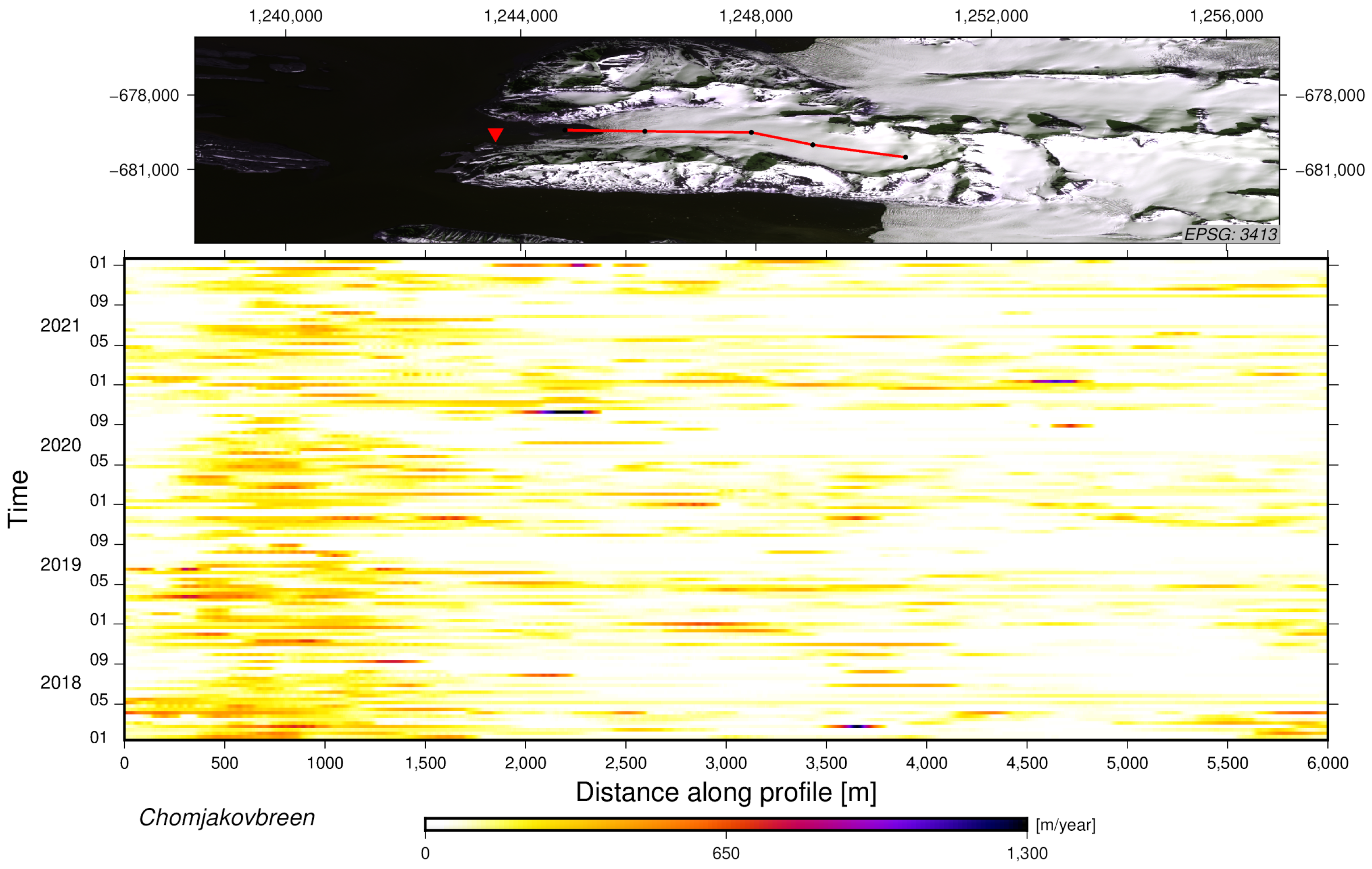
Figure A1.
Temporal evolution of the Chomjakovbreen flow velocity for the period from December 2018 to January 2022 (calculated as velocities per year) along the profile marked with a red line in the Sentinel 2 satellite image. The red triangle indicates the location of the meteorological data measurements, shown in
Figure 10. The background image (top) is the Sentinel 2 image acquired in 6 July 2018 and displayed in NSIDC Sea Ice Polar Stereographic North (EPSG:3413).
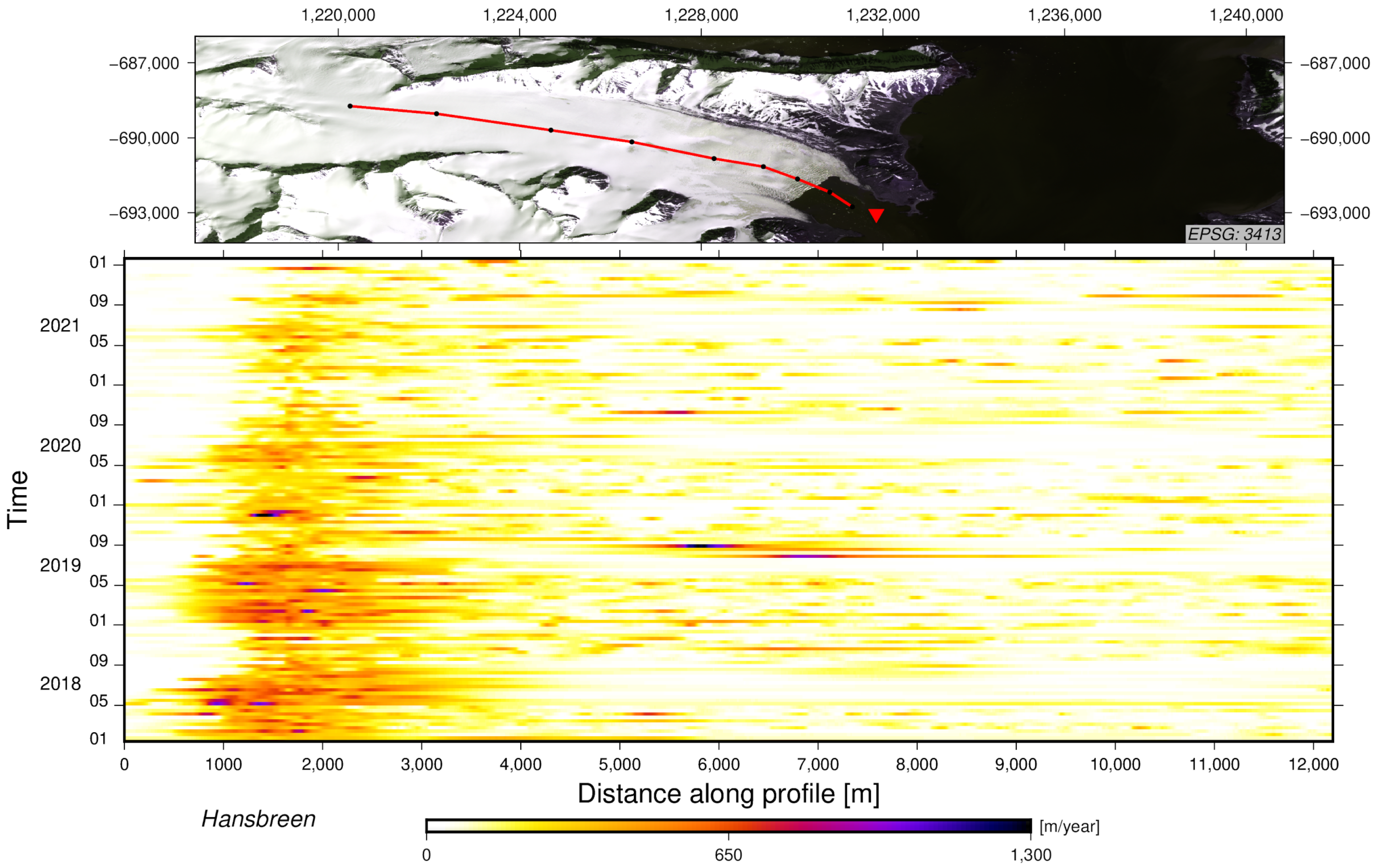
Figure A2.
Temporal evolution of the Hansbreen flow velocity for the period from December 2018 to January 2022 (calculated as velocities per year) along the profile marked with a red line in the Sentinel 2 satellite image. The red triangle indicates the location of the meteorological data measurements, shown in
Figure 10. The background image (top) is the Sentinel 2 image acquired in 6 July 2018 and displayed in NSIDC Sea Ice Polar Stereographic North (EPSG:3413).
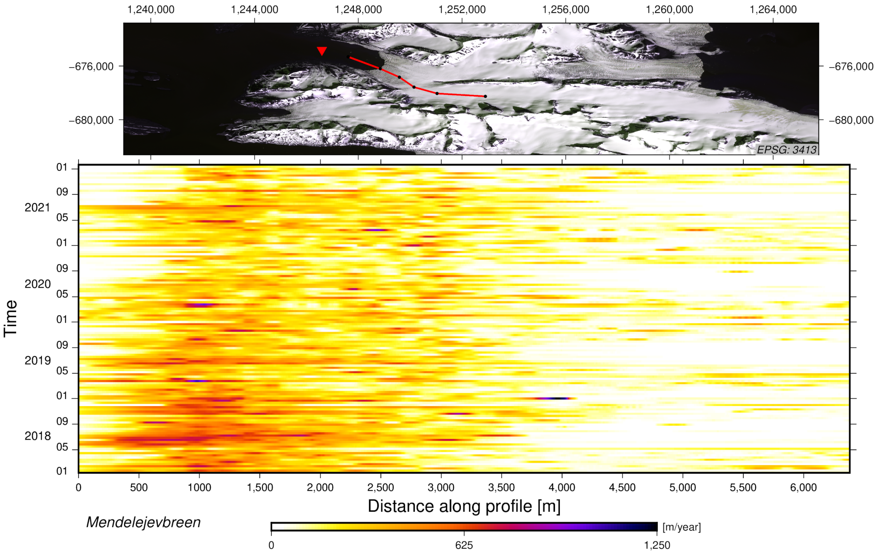
Figure A3.
Temporal evolution of the Mmendelejevbreen flow velocity for the period from December 2018 to January 2022 (calculated as velocities per year) along the profile marked with a red line in the Sentinel 2 satellite image. The red triangle indicates the location of the meteorological data measurements, shown in
Figure 10. The background image (top) is the Sentinel 2 image acquired in 6 July 2018 and displayed in NSIDC Sea Ice Polar Stereographic North (EPSG:3413).
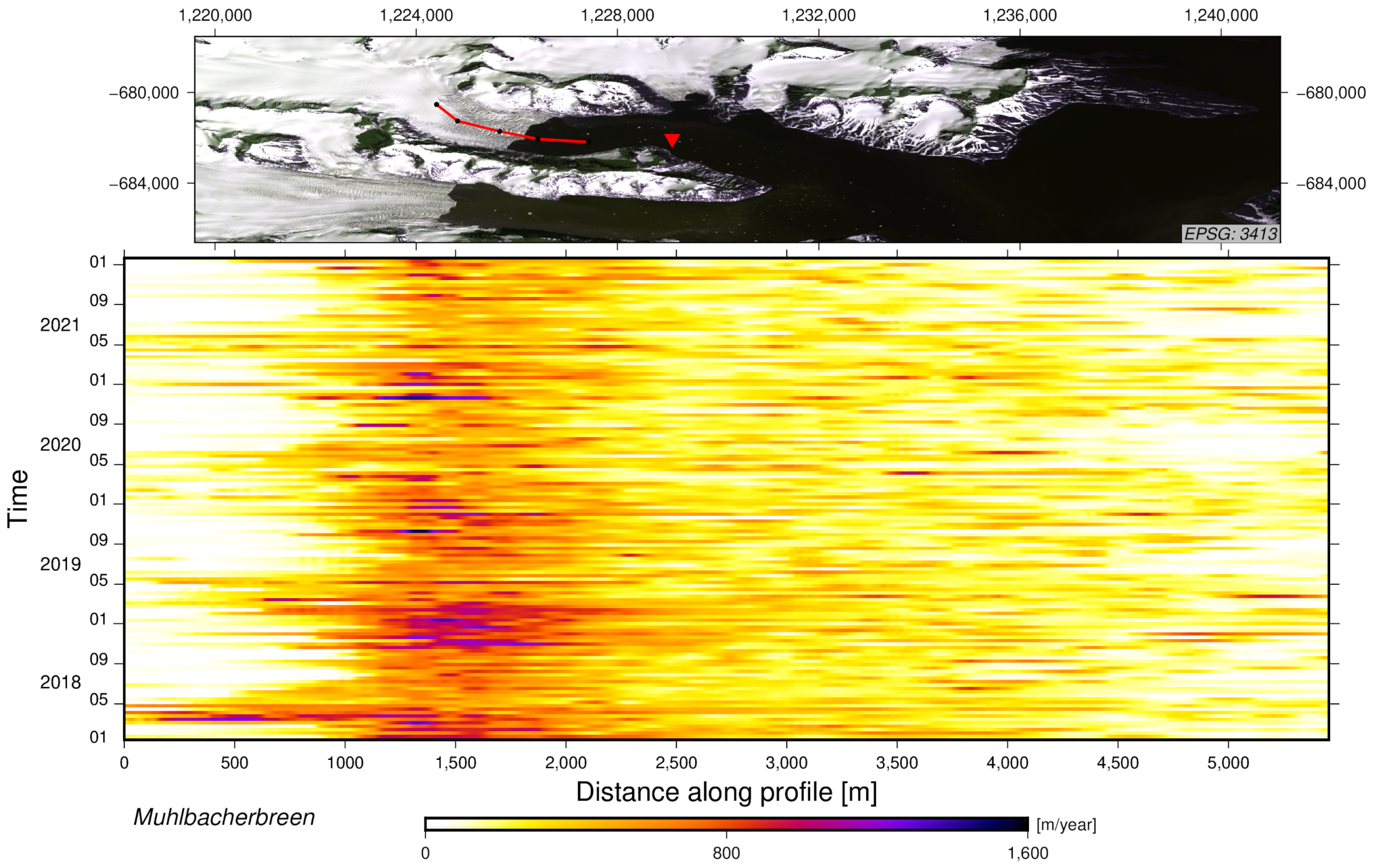
Figure A4.
Temporal evolution of the Muhlbacherbreen flow velocity for the period December 2018 to January 2022 (calculated as velocities per year) along the profile marked with a red line in the Sentinel 2 satellite image. The red triangle indicates the location of the meteorological data measurements, shown in
Figure 10. The background image (top) is the Sentinel 2 image acquired in 6 July 2018 and displayed in NSIDC Sea Ice Polar Stereographic North (EPSG:3413).
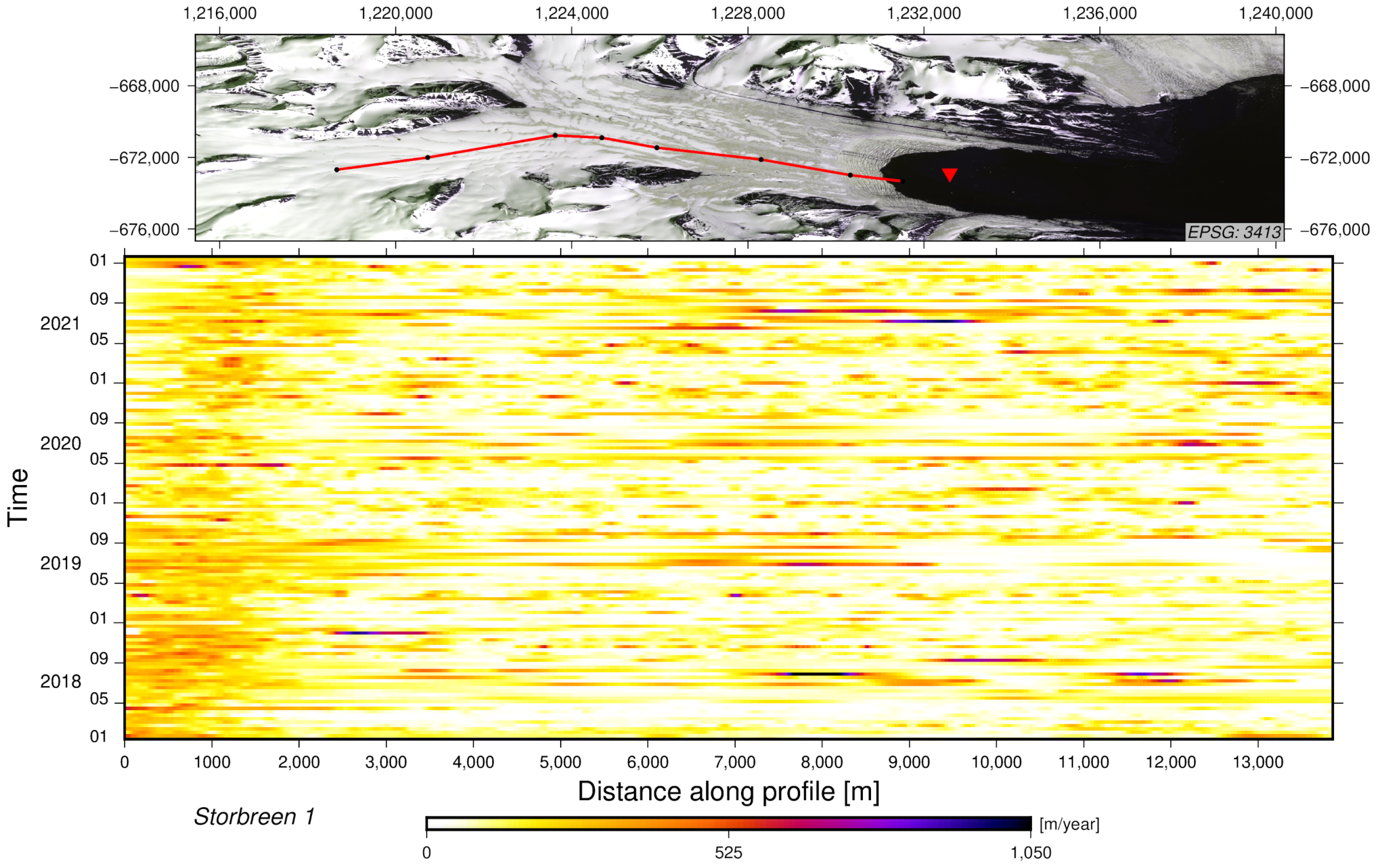
Figure A5.
Temporal evolution of the Storbreen flow velocity for the period from December 2018 to January 2022 (calculated as velocities per year) along the profile marked with a red line in the Sentinel 2 satellite image. The red triangle indicates the location of the meteorological data measurements, shown in
Figure 10. The background image (top) is the Sentinel 2 image acquired in 6 July 2018 and displayed in NSIDC Sea Ice Polar Stereographic North (EPSG:3413).
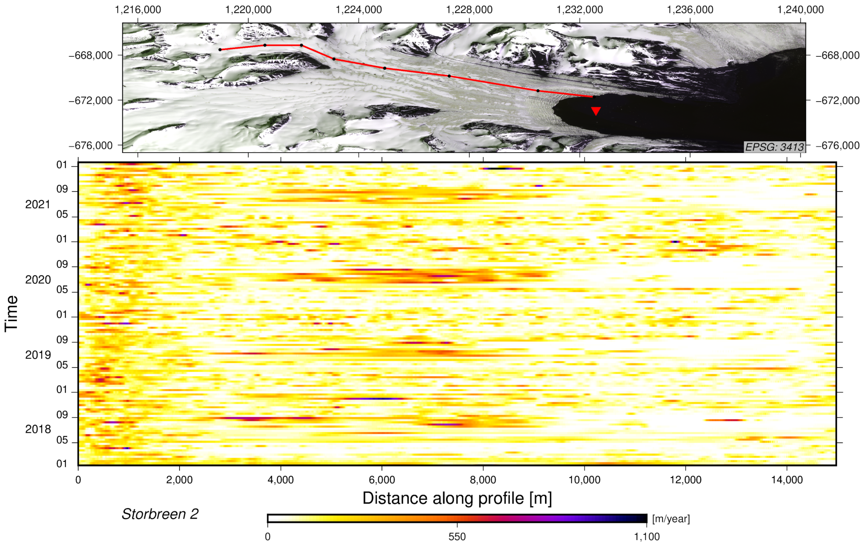
Figure A6.
Temporal evolution of the Storbreen flow velocity for the period from December 2018 to January 2022 (calculated as velocities per year) along the profile marked with a red line in the Sentinel 2 satellite image. The red triangle indicates the location of the meteorological data measurements, shown in
Figure 10. The background image (top) is the Sentinel 2 image acquired in 6 July 2018 and displayed in NSIDC Sea Ice Polar Stereographic North (EPSG:3413).
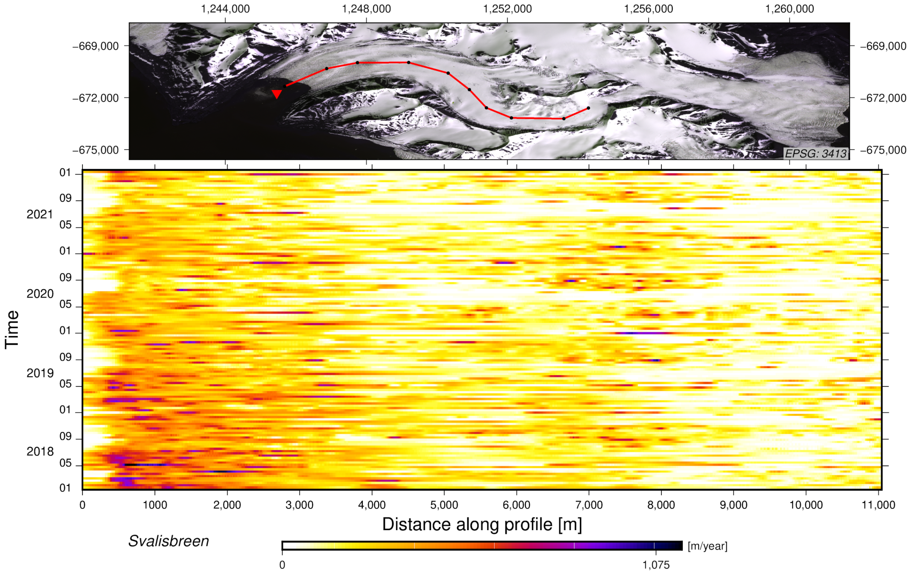
Figure A7.
Temporal evolution of the Svalisbreen flow velocity for the period from December 2018 to January 2022 (calculated as velocities per year) along the profile marked with a red line in the Sentinel 2 satellite image. The red triangle indicates the location of the meteorological data measurements, shown in
Figure 10. The background image (top) is the Sentinel 2 image acquired in 6 July 2018 and displayed in NSIDC Sea Ice Polar Stereographic North (EPSG:3413).
Appendix A.2
Table A1.
List of used SAR images from Sentinel 1A/B missions.
Table A1.
List of used SAR images from Sentinel 1A/B missions.
| Spaceborne Sensor | Acquisition Date, Path 14 |
|---|
| | 20180106; 20180118; 20180130; 20180211; 20180223; 20180307; 20180319; 20180331; |
| | 20180412; 20180424; 20180506; 20180518; 20180530; 20180611; 20180623; 20180705; |
| | 20180717; 20180729; 20180810; 20180822; 20180903; 20180915; 20180927; 20181009; |
| | 20181021; 20181102; 20181114; 20181126; 20181208; 20181220; 20190101; 20190113; |
| | 20190125; 20190206; 20190218; 20190302; 20190314; 20190326; 20190407; 20190419; |
| | 20190501; 20190513; 20190525; 20190606; 20190618; 20190630; 20190712; 20190724; |
| Sentinel 1A | 20190805; 20190817; 20190829; 20190910; 20190922; 20191004; 20191016; 20191028; |
| | 20191109; 20191121; 20191215; 20191227; 20200108; 20200120; 20200201; 20200213; |
| | 20200225; 20200308; 20200320; 20200401; 20200413; 20200425; 20200507; 20200519; |
| | 20200531; 20200612; 20200624; 20200706; 20200718; 20200730; 20200811; 20200823; |
| | 20200904; 20200916; 20200928; 20201010; 20201022; 20201115; 20201127; 20201209; |
| | 20201221; 20210102; 20210114; 20210126; 20210207; 20210219; 20210303; 20210315; |
| | 20210327; 20210408; 20210420; 20210502; 20210514; 20210526; 20210607; 20210619; |
| | 20210701; 20210725; 20210806; 20210818; 20210830; 20210911; 20210923; 20211005; |
| | 20211017; 20211029; 20211110; 20211122; 20211216; 20211228; 20220109; 20220121 |
| | 20180112; 20180124; 20180205; 20180217; 20180301; 20180313; 20180325; 20180406; |
| | 20180418; 20180430; 20180512; 20180524; 20180605; 20180617; 20180629; 20180711; |
| | 20180723; 20180804; 20180816; 20180828; 20180909; 20180921; 20181003; 20181015; |
| | 20181027; 20181108; 20181120; 20181202; 20181214; 20181226; 20190107; 20190119; |
| | 20190131; 20190212; 20190224; 20190308; 20190320; 20190401; 20190413; 20190425; |
| | 20190507; 20190519; 20190531; 20190612; 20190624; 20190706; 20190718; 20190730; |
| | 20190811; 20190823; 20190904; 20190916; 20190928; 20191010; 20191022; 20191103; |
| Sentinel 1A | 20191115; 20191127; 20191209; 20191221; 20200102; 20200114; 20200126; 20200207; |
| | 20200219; 20200302; 20200314; 20200326; 20200407; 20200419; 20200501; 20200513; |
| | 20200525; 20200606; 20200618; 20200630; 20200712; 20200724; 20200805; 20200817; |
| | 20200829; 20200910; 20200922; 20201004; 20201016; 20201028; 20201109; 20201121; |
| | 20201203; 20201215; 20201227; 20210108; 20210120; 20210201; 20210213; 20210225; |
| | 20210309; 20210321; 20210402; 20210414; 20210426; 20210508; 20210520; 20210601; |
| | 20210613; 20210625; 20210707; 20210719; 20210731; 20210812; 20210824; 20210905; |
| | 20210917; 20210929; 20211011; 20211023; 20211104; 20211116; 20211128; 20211210; |
| | 20211222; |
References
- Vaughan, D.; Comiso, J.; Allison, I.; Carrasco, J.; Kaser, G.; Kwok, R.; Mote, P.; Murray, T.; Paul, F.; Ren, J.; et al. Observations: Cryosphere; Cambridge University Press: Cambridge, UK; New York, NY, USA, 2013; Volume 10, pp. 317–382. [Google Scholar]
- Małecki, J. Accelerating Retreat and High-Elevation Thinning of Glaciers in Central Spitsbergen. Cryosphere 2016, 10, 1317–1329. [Google Scholar] [CrossRef] [Green Version]
- Błaszczyk, M.; Jania, J.A.; Hagen, J.O. Tidewater glaciers of Svalbard: Recent changes and estimates of calving fluxes. Pol. Polar Res. 2009, 30, 85–142. [Google Scholar]
- Błaszczyk, M.; Jania, J.; Kolondra, L. Fluctuations of Tidewater Glaciers in Hornsund Fjord (Southern Svalbard) since the Beginning of the 20th Century. Pol. Polar Res. 2013, 34, 327–352. [Google Scholar] [CrossRef]
- Ignatiuk, D.; Błaszczyk, M.; Budzik, T.; Grabiec, M.; Jania, J.A.; Kondracka, M.; Laska, M.; Małarzewski, L.; Stachnik, L. A Decade of Glaciological and Meteorological Observations in the Arctic (Werenskioldbreen, Svalbard). Earth Syst. Sci. Data 2022, 14, 2487–2500. [Google Scholar] [CrossRef]
- Fürst, J.J.; Gillet-Chaulet, F.; Benham, T.J.; Dowdeswell, J.A.; Grabiec, M.; Navarro, F.; Pettersson, R.; Moholdt, G.; Nuth, C.; Sass, B.; et al. Application of a two-step approach for mapping ice thickness to various glacier types on Svalbard. Cryosphere 2017, 11, 2003–2032. [Google Scholar] [CrossRef] [Green Version]
- Noël, B.; Jakobs, C.L.; Van Pelt, W.; Lhermitte, S.; Wouters, B.; Kohler, J.; Hagen, J.O.; Luks, B.; Reijmer, C.; Van de Berg, W.J.; et al. Low elevation of Svalbard glaciers drives high mass loss variability. Nat. Commun. 2020, 11, 4597. [Google Scholar] [CrossRef]
- Strozzi, T.; Wiesmann, A.; Kääb, A.; Schellenberger, T.; Paul, F. Ice Surface Velocity in the Eastern Arctic from Historical Satellite SAR Data. Earth Syst. Sci. Data Discuss. 2022, 2022, 1–42. [Google Scholar] [CrossRef]
- Barzycka, B.; Grabiec, M.; Błaszczyk, M.; Ignatiuk, D.; Laska, M.; Hagen, J.O.; Jania, J. Changes of glacier facies on Hornsund glaciers (Svalbard) during the decade 2007–2017. Remote Sens. Environ. 2020, 251, 112060. [Google Scholar] [CrossRef]
- Mohajerani, Y.; Jeong, S.; Scheuchl, B.; Velicogna, I.; Rignot, E.; Milillo, P. Automatic Delineation of Glacier Grounding Lines in Differential Interferometric Synthetic-Aperture Radar Data Using Deep Learning. Sci. Rep. 2021, 11, 4992. [Google Scholar] [CrossRef] [PubMed]
- Joughin, I.R.; Winebrenner, D.P.; Fahnestock, M.A. Observations of ice-sheet motion in Greenland using satellite radar interferometry. Geophys. Res. Lett. 1995, 22, 571–574. [Google Scholar] [CrossRef]
- Mouginot, J.; Rignot, E.; Scheuchl, B. Continent-Wide, Interferometric SAR Phase, Mapping of Antarctic Ice Velocity. Geophys. Res. Lett. 2019, 46, 9710–9718. [Google Scholar] [CrossRef]
- Lei, Y.; Gardner, A.S.; Agram, P. Processing methodology for the ITS_LIVE Sentinel-1 ice velocity product. Earth Syst. Sci. Data Discuss. 2021, 2021, 1–27. [Google Scholar] [CrossRef]
- Strozzi, T.; Luckman, A.; Murray, T.; Wegmuller, U.; Werner, C. Glacier motion estimation using SAR offset-tracking procedures. IEEE Trans. Geosci. Remote Sens. 2002, 40, 2384–2391. [Google Scholar] [CrossRef] [Green Version]
- Kumar, V.; Venkataraman, G.; Rao, Y.S. SAR interferometry and Speckle tracking approach for glacier velocity estimation using ERS-1/2 and TerraSAR-X spotlight high resolution data. In Proceedings of the 2009 IEEE International Geoscience and Remote Sensing Symposium, Cape Town, South Africa, 12–17 July 2009; Volume 5, pp. V-332–V-335. [Google Scholar] [CrossRef]
- Gardner, A.S.; Moholdt, G.; Scambos, T.; Fahnstock, M.; Ligtenberg, S.; van den Broeke, M.; Nilsson, J. Increased West Antarctic and unchanged East Antarctic ice discharge over the last 7 years. Cryosphere 2018, 12, 521–547. [Google Scholar] [CrossRef] [Green Version]
- Nagler, T.; Rott, H.; Hetzenecker, M.; Wuite, J.; Potin, P. The Sentinel-1 Mission: New Opportunities for Ice Sheet Observations. Remote Sens. 2015, 7, 9371–9389. [Google Scholar] [CrossRef] [Green Version]
- Mouginot, J.; Rignot, E.; Scheuchl, B.; Wood, M.; Millan, R. Annual Ice Velocity of the Greenland Ice Sheet (2001–2010); Dryad: Davis, CA, USA, 2019. [Google Scholar] [CrossRef]
- Joughin, I. MEaSUREs Greenland Ice Velocity Annual Mosaics from SAR and Landsat, Version 2; NSIDC: Boulder, CO, USA, 2020. [Google Scholar] [CrossRef]
- Solgaard, A.; Kusk, A.; Merryman Boncori, J.P.; Dall, J.; Mankoff, K.D.; Ahlstrøm, A.P.; Andersen, S.B.; Citterio, M.; Karlsson, N.B.; Kjeldsen, K.K.; et al. Greenland ice velocity maps from the PROMICE project. Earth Syst. Sci. Data 2021, 13, 3491–3512. [Google Scholar] [CrossRef]
- Friedl, P.; Seehaus, T.; Braun, M. Sentinel-1 Ice Surface Velocities of Svalbard; GFZ Data Services: Potsdam, Germany, 2021. [Google Scholar] [CrossRef]
- Isaksen, K.; Nordli, O.; Førland, E.J.; Łupikasza, E.; Eastwood, S.; Niedźwiedź, T. Recent warming on Spitsbergen—Influence of atmospheric circulation and sea ice cover. J. Geophys. Res. Atmos. 2016, 121, 11913–11931. [Google Scholar] [CrossRef]
- Geyman, E.C.; van Pelt, W.J.J.; Maloof, A.C.; Aas, H.F.; Kohler, J. Historical Glacier Change on Svalbard Predicts Doubling of Mass Loss by 2100. Nature 2022, 601, 374–379. [Google Scholar] [CrossRef]
- Nuth, C.; Kohler, J.; König, M.; von Deschwanden, A.; Hagen, J.O.; Kääb, A.; Moholdt, G.; Pettersson, R. Decadal changes from a multi-temporal glacier inventory of Svalbard. Cryosphere 2013, 7, 1603–1621. [Google Scholar] [CrossRef] [Green Version]
- Jania, J. Klasyfikacja i Cechy Morfometryczne Lodowców Otoczenia Hornsundu, Spitsbergen; Uniwersytet Śląski: Katowice, Poland, 1988. [Google Scholar]
- Martín-Moreno, R.; Allende Álvarez, F.; Hagen, J.O. ‘Little Ice Age’ Glacier Extent and Subsequent Retreat in Svalbard Archipelago. Holocene 2017, 27, 1379–1390. [Google Scholar] [CrossRef]
- Strzelecki, M.C.; Szczuciński, W.; Dominiczak, A.; Zagórski, P.; Dudek, J.; Knight, J. New Fjords, New Coasts, New Landscapes: The Geomorphology of Paraglacial Coasts Formed after Recent Glacier Retreat in Brepollen (Hornsund, Southern Svalbard). Earth Surf. Process. Landforms 2020, 45, 1325–1334. [Google Scholar] [CrossRef] [Green Version]
- Błaszczyk, M.; Ignatiuk, D.; Uszczyk, A.; Cielecka-Nowak, K.; Grabiec, M.; Jania, J.A.; Moskalik, M.; Walczowski, W. Freshwater Input to the Arctic Fjord Hornsund (Svalbard). Polar Res. 2019. [Google Scholar] [CrossRef]
- Rosen, P.A.; Gurrola, E.; Sacco, G.F.; Zebker, H. The InSAR scientific computing environment. In Proceedings of the EUSAR 2012—9th European Conference on Synthetic Aperture Radar, Nuremberg, Germany, 23–26 April 2012; pp. 730–733. [Google Scholar]
- Porter, C.; Morin, P.; Howat, I.; Noh, M.J.; Bates, B.; Peterman, K.; Keesey, S.; Schlenk, M.; Gardiner, J.; Tomko, K.; et al. ArcticDEM; Harvard Dataverse: Thessaloniki, Greece, 2018. [Google Scholar] [CrossRef]
- Copernicus Climate Change Service. Arctic Regional Reanalysis on Single Levels from 1991 to Present; Copernicus Climate Change Service: Sherfield, UK, 2021. [Google Scholar] [CrossRef]
- Polish Polar Station Institute of Geophysics Polish Academy of Sciences. Meteorological Bulletin—Spitsbergen—Hornsund, 2014–2021. Available online: https://hornsund.igf.edu.pl/Biuletyny/ (accessed on 17 August 2022).
- Lei, Y.; Gardner, A.; Agram, P. Autonomous Repeat Image Feature Tracking (autoRIFT) and Its Application for Tracking Ice Displacement. Remote Sens. 2021, 13, 749. [Google Scholar] [CrossRef]
- Bindschadler, R.A.; Scambos, T.A. Satellite-Image-Derived Velocity Field of an Antarctic Ice Stream. Science 1991, 252, 242–246. [Google Scholar] [CrossRef] [Green Version]
- Institute, N.P. Kartdata Svalbard 1:100,000 (S100 Kartdata)/Map Data; Norwegian Polar Institute: Tromsø, Norway, 2014. [Google Scholar] [CrossRef]
- Paul, F.; Bolch, T.; Briggs, K.; Kääb, A.; McMillan, M.; McNabb, R.; Nagler, T.; Nuth, C.; Rastner, P.; Strozzi, T.; et al. Error sources and guidelines for quality assessment of glacier area, elevation change, and velocity products derived from satellite data in the Glaciers-cci project. Remote Sens. Environ. 2017, 203, 256–275. [Google Scholar] [CrossRef] [Green Version]
- Riel, B.; Minchew, B.; Joughin, I. Observing traveling waves in glaciers with remote sensing: New flexible time series methods and application to Sermeq Kujalleq (Jakobshavn Isbræ), Greenland. Cryosphere 2021, 15, 407–429. [Google Scholar] [CrossRef]
- Schuler, T.V.; Kohler, J.; Elagina, N.; Hagen, J.O.M.; Hodson, A.J.; Jania, J.A.; Kääb, A.M.; Luks, B.; Małecki, J.; Moholdt, G.; et al. Reconciling Svalbard glacier mass balance. Front. Earth Sci. 2020, 8, 156. [Google Scholar] [CrossRef]
- Błaszczyk, M.; Jania, J.A.; Ciepły, M.; Grabiec, M.; Ignatiuk, D.; Kolondra, L.; Kruss, A.; Luks, B.; Moskalik, M.; Pastusiak, T.; et al. Factors Controlling Terminus Position of Hansbreen, a Tidewater Glacier in Svalbard. J. Geophys. Res. Earth Surf. 2021, 126, e2020JF005763. [Google Scholar] [CrossRef]
Figure 1.
Svalbard—the study area: (Svalbard—the study area: (a) the archipelago with an outline of scenes from the ascending path 14, (b) the Hornsund fiord anf the analyzed glaciers. Light blue areas indicate ice cover, blue areas—lakes and brown areas—moraines.
Figure 1.
Svalbard—the study area: (Svalbard—the study area: (a) the archipelago with an outline of scenes from the ascending path 14, (b) the Hornsund fiord anf the analyzed glaciers. Light blue areas indicate ice cover, blue areas—lakes and brown areas—moraines.
Figure 2.
Data processing flowchart,(a) part concerning the ISCE processing, (b) Geogrid processing, (c) autoRIFT processing.
Figure 2.
Data processing flowchart,(a) part concerning the ISCE processing, (b) Geogrid processing, (c) autoRIFT processing.
Figure 3.
Input data visualisation, (a) reference velocity in X direction, (b) DEM, (c) slope in X direction, (d) chip size for X direction, (e) search limit, (f) stable surface.
Figure 3.
Input data visualisation, (a) reference velocity in X direction, (b) DEM, (c) slope in X direction, (d) chip size for X direction, (e) search limit, (f) stable surface.
Figure 4.
Reference area (green) for MAD values calculations.
Figure 4.
Reference area (green) for MAD values calculations.
Figure 5.
Mean ice flow velocities for glaciers surrounding Hornsund bay: (a) 2018, (b) 2019, (c) 2020, (d) 2021 year. The numbers in brackets identify the following glaciers: (1) Hansbreen, (2) Paierlbreen, (3) Muhlbacherbreen, (4) Storbreen, (5) Hornbreen, (6) Svalisbreen, (7) Mendelejevbreen, (8) Chomjakovbreen, (9) Samarinbreen.
Figure 6.
Temporal evolution of the Paierlbreen flow velocity for the period from December 2018 to January 2022 (calculated as velocities in meters per year) along the profile marked with a red line in the Sentinel 2 satellite image. The red triangle indicates the location of the meteorological data measurements. The background image (top) is a Sentinel 2 image acquired in 6 July 2018 and displayed in NSIDC Sea Ice Polar Stereographic North (EPSG:3413).
Figure 7.
Temporal evolution of the Hornbreen flow velocity for the period from December 2018 to January 2022 (calculated as velocities in meters per year) along the profile marked with a red line in the Sentinel 2 satellite image. The red triangle indicates the location of the meteorological data measurements. The background image (top) is the Sentinel 2 image acquired in 6 July 2018 and displayed in NSIDC Sea Ice Polar Stereographic North (EPSG:3413).
Figure 8.
Temporal evolution of the Samarinbreen flow velocity for the period from December 2018 to January 2022 (calculated as velocities in meters per year) along the profile marked with a red line in the Sentinel 2 satellite image. The red triangle indicates the location of the meteorological data measurements. The background image (top) is the Sentinel 2 image acquired in 6 July 2018 and displayed in NSIDC Sea Ice Polar Stereographic North (EPSG:3413).
Figure 9.
Location of measurement points (top) and below time series for ice flow velocities in NSIDC Polar Stereographic North (EPSG:3411). The background image (top) is the Sentinel 2 image acquired in 6 July 2018. Red-and-white circles indicate the points for all analysed glaciers at the Hornsund Bay surroundings from which the data shown in the graphs below were taken. Each plot shows the seasonal variation in MAD values (solid red line), as well as the long-term velocity model [
37] results (solid dark lines) while blue dots indicate observed values. The grey stripes mark the summer periods (June–September).
Figure 10.
Summary of ice mass velocities in relation to meteorological data for points (represented by red-and-white triangles) located in the region of the front of the analyzed glaciers. For 2021, meteorological data are provided by the end of June—values marked with *. The background image (top) is the Sentinel 2 image acquired in 6 July 2018 (displayed in NSIDC Polar Stereographic North (EPSG:3411)). Detailed description of the presented data is provided in the lower right corner of the figure.
Table 1.
Glaciers of Hornsund fiord with morphological characteristics and morphometric features.
Table 1.
Glaciers of Hornsund fiord with morphological characteristics and morphometric features.
| Name | GLIMS ID | Morphological
Characteristics [25] | Area
[km] [4] | Aspect [4] | Slope
(Centerline) [4] | Slope
(Surface) [4] |
|---|
| Hansbreen | G015592E77097N | semi-cap | 53.9 | S | 1.7 | 1.1 |
| Paierlbreen | G015696E77195N | semi-cap | 106.1 | S | 1.7 | 7.4 |
| Muhlbacher-breen | G015900E77167N | complex | 51.6 | SE | 2.2 | 7.6 |
| Storbreen | G016172E77192N | complex | 196.5 | S | 1.3 | 6.1 |
| Hornbreen | G016807E77171N | semi-cap, complex | 176.2 | SW | 1.3 | 6.1 |
| Svalisbreen | G016777E76955N | | 31.3 | NW | 1.9 | 5.8 |
| Mendelejev-breen | G016557E76915N | semi-cap, | 31.1 | N | 1.9 | 7.1 |
| Chomjakov-breen | G016435E76929N | complex | 13.1 | NW | 4.0 | 9.6 |
| Samarin-breen | G016221E76879N | complex dual-flow | 84.0 | NW | 1.7 | 9.0 |
Table 3.
Statistics for time series of Sentinel 1 velocity 2018–2021 for selected glaciers in Hornsund Fjord. Including annual median, maximum, minimum and median values for summer (June–September) and winter (October–May) periods. All values are presented in m/year.
Table 3.
Statistics for time series of Sentinel 1 velocity 2018–2021 for selected glaciers in Hornsund Fjord. Including annual median, maximum, minimum and median values for summer (June–September) and winter (October–May) periods. All values are presented in m/year.
| Year | Chomjakovbreen | Hansbreen | Hornbreen | Mendelejevbreen | Muhlbacherbreen | Paierlbreen | Samarinbreen | Storbreen | Svalisbreen |
|---|
| 2018 | 207 | 405 | 461 | 530 | 732 | 829 | 143 | 165 | 467 |
| 2018 | 613 | 803 | 898 | 929 | 1394 | 1213 | 516 | 373 | 1244 |
| 2018 | 3 | 19 | 115 | 102 | 359 | 268 | 20 | 29 | 35 |
| winter | 243 | 449 | 495 | 513 | 734 | 1014 | 155 | 141 | 647 |
| summer | 201 | 420 | 428 | 464 | 570 | 681 | 153 | 156 | 349 |
| 2019 | 144 | 407 | 431 | 380 | 674 | 753 | 193 | 179 | 430 |
| 2019 | 670 | 927 | 901 | 652 | 1152 | 1315 | 765 | 509 | 995 |
| 2019 | 13 | 52 | 100 | 123 | 124 | 102 | 0 | 27 | 65 |
| winter | 158 | 279 | 338 | 306 | 508 | 522 | 184 | 130 | 347 |
| summer | 165 | 419 | 540 | 409 | 682 | 882 | 223 | 209 | 446 |
| 2020 | 157 | 269 | 423 | 271 | 500 | 461 | 182 | 148 | 312 |
| 2020 | 549 | 626 | 857 | 744 | 983 | 971 | 718 | 439 | 1033 |
| 2020 | 15 | 21 | 149 | 96 | 197 | 32 | 7 | 31 | 40 |
| winter | 158 | 279 | 338 | 306 | 508 | 522 | 184 | 130 | 347 |
| summer | 201 | 348 | 518 | 276 | 570 | 518 | 243 | 165 | 331 |
| 2021 | 180 | 189 | 400 | 310 | 496 | 338 | 204 | 212 | 344 |
| 2021 | 498 | 650 | 1295 | 905 | 998 | 734 | 755 | 642 | 957 |
| 2021 | 5 | 14 | 63 | 80 | 116 | 16 | 7 | 47 | 0 |
| winter | 192 | 152 | 292 | 278 | 474 | 192 | 140 | 256 | 338 |
| summer | 203 | 242 | 526 | 372 | 517 | 437 | 295 | 222 | 334 |
| Publisher’s Note: MDPI stays neutral with regard to jurisdictional claims in published maps and institutional affiliations. |
© 2022 by the authors. Licensee MDPI, Basel, Switzerland. This article is an open access article distributed under the terms and conditions of the Creative Commons Attribution (CC BY) license (https://creativecommons.org/licenses/by/4.0/).


