Machine Learning and Hyperparameters Algorithms for Identifying Groundwater Aflaj Potential Mapping in Semi-Arid Ecosystems Using LiDAR, Sentinel-2, GIS Data, and Analysis

Abstract

Aflaj (plural of falaj) are tunnels or trenches built to deliver groundwater from its source to the point of consumption. Support vector machine (SVM) and extreme gradient boosting (XGB) machine learning models were used to predict groundwater aflaj potential in the Nizwa watershed in the Sultanate of Oman (Oman). Nizwa city is a focal point of aflaj that underlies the historical relationship between ecology, economic dynamics, agricultural systems, and human settlements. Three hyperparameter algorithms, grid search (GS), random search (RS), and Bayesian optimisation, were used to optimise the parameters of the XGB model. Sentinel-2 and light detection and ranging (LiDAR) data via geographical information systems (GIS) were employed to derive variables of land use/land cover, and hydrological, topographical, and geological factors. The groundwater aflaj potential maps were categorised into five classes: deficient, low, moderate, high, and very high. Based on the evaluation of accuracy in the training stage, the following models showed a high level of accuracy based on the area under the curve: Bayesian-XGB (0.99), GS-XGB (0.97), RS-XGB (0.96), SVM (0.96), and XGB (0.93). The validation results showed that the Bayesian hyperparameter algorithm significantly increased XGB model efficiency in modelling groundwater aflaj potential. The highest percentages of groundwater potential in the very high class were the XGB (10%), SVM (8%), GS-XGB (6%), RS-XGB (6%), and Bayesian-XGB (6%) models. Most of these areas were located in the central and northeast parts of the case study area. The study concluded that evaluating existing groundwater datasets, facilities, current, and future spatial datasets is critical in order to design systems capable of mapping groundwater aflaj based on geospatial and ML techniques. In turn, groundwater protection service projects and integrated water source management (IWSM) programs will be able to protect the aflaj irrigation system from threats by implementing timely preventative measures.

1. Introduction

Groundwater is critical to many countries’ livelihoods and economic survival. However, this hidden resource suffers from a lack of adequate management [1,2]. Groundwater levels have been reported to be exhausted, and groundwater quality negatively impacts both developed and underdeveloped countries [3]. In addition to exhaustion in some areas, rising groundwater levels in other arid and semi-arid zones represent a significant risk to ecological systems. To safeguard the long-term resilience of this subsurface resource, a complex problem under an expanding population and climate change, there is an immediate need for efficient and effective management. Nevertheless, people in the Sultanate of Oman (Oman), a developing nation, have historically adapted to arid conditions with little or no surface water. Aflaj (plural for falaj) are trenches or tunnels built to transport groundwater from their source to the point of consumption in the country. Omanis developed a means to reach groundwater by digging horizontal underground channels, known as aflaj. Aflaj became the typical approach to groundwater abstraction, consisting of channels and hydraulic structures for intercepting and distributing water for irrigation and residential use [4]. These gravity-powered water networks, which transport water from sources to areas of demand [5], have been in use for thousands of years and currently represent more than one-third of the water consumed by agriculture. Aflaj irrigation systems are used in more than 34 nations worldwide [6]. The system of aflaj is often likened to the qanat irrigation system used in Iran in the Persian era about 3000 years ago. The aflaj irrigation systems included in this inventory were divided into three categories recognised in Oman: Iddi (Dawoodi), Ayni, and Ghaili [7]. The most sophisticated form is Daudi falaj, which taps groundwater from 10–30 m below ground to use at the surface without pumping (https://www.maf.gov.om/, accessed on 30 May 2022). The falaj channel begins in the continuously saturated zone and continues underground in a down-gradient direction until it reaches the earth’s surface. The ability to carry out hydraulic leveling and excavate the falaj tunnels beneath the earth on rocky terrain with crude instruments exemplified aflaj building genius. The two varieties, Ainiy and Ghaily aflaj are simple canalisations of groundwater flowing on the surface naturally or coming out of a spring and running it till it finds a suitable area for cultivation. Through these systems water flowing from the falaj is managed wisely by a committee representing the owners of that particular falaj. A total of 23% were Iddi, 28% were Ayni and 49% were Ghaili.

Notably, the aflaj irrigation systems in Oman have been under threat due to groundwater pumping and economic development since 1970 [8,9]. Thus, groundwater levels, including those for aflaj systems, have plummeted in recent decades around the world, including Oman, due to excessive water extraction rates and ineffective management [6]. Therefore, Oman has limited annual rainfall, and the effects of climate change are likely to worsen the situation. As a result, over 1000 aflaj are deemed dry or dead. Maintaining active aflaj is a huge task that is nearly impossible for one party to accomplish alone. In Oman, the main source of water is rain, which recharges ground aquifers; there is no surface water in the country, and rain in most arid regions is highly variable in terms of time, duration, quality, and space.

Groundwater, which flows through the soil and protects the water level in rivers, lakes, and wetlands, is especially important during dry seasons when direct rainwater recharge is low. This helps to preserve wildlife and plants, and its role in keeping water levels stable during dry seasons helps to keep marine travel moving along inland waters and rivers. Water is stored in deeper layers beneath the earth’s surface, which preserves its quality and protects it from pollution, making it suitable for direct consumption without high extraction or treatment costs, but it is critical to preserve this vital importance due to depletion or pollution [10]. Therefore, assessing groundwater aflaj potential is critical for maintaining groundwater resources, especially in data-scarce areas. To conduct an assessment, machine learning techniques are needed to analyze the critical groundwater conditioning factors for groundwater aflaj potential mapping.

The commonly used methods for detecting groundwater resources, including aflaj, are flawed because they are complex, uneconomical, time-consuming, expensive, and occasionally unreliable. Given these flaws, groundwater resources must be re-evaluated using innovative technologies, such as artificial intelligence (AI), machine learning (ML), global positioning systems (GPS), remote sensing, and geographic information systems (GIS). While satellite and airborne sensors have limited applications in groundwater surveys, they provide valuable insights into specific hydrogeological processes and variables, especially when combined with other datasets. Remote sensing data are instrumental in developing countries, where hydrogeological monitoring is rarely structured, and the potential for groundwater resources is mainly unknown [11]. Remote sensing has recently emerged as a critical tool in environmental management. Visual images can be examined and interpreted to monitor the quality and quantity of water resources and their geographic distribution. In conjunction with selected field observations, visual picture interpretation is an effective method for mapping groundwater potential. In addition, high-resolution satellite-mounted infrared sensors can provide data analysis of water stored in small reservoirs in arid and semi-arid regions. These technologies have made groundwater assessment and determining groundwater potential more cost-effective [12,13]. Thus, managers may be assisted in developing optimum water resource management scenarios through groundwater assessments. The presence of groundwater in any location on Earth results from a combination of climatic, geological, hydrological, physiographic, and ecological factors [14]. Additional influencing factors include terrain, lithology, geological formations, and slope [15]. By studying these parameters, groundwater aflaj potential maps for a basin can be developed using several spatial approaches.

GIS provides numerous options for hydrological modelling, including spatially distributed models of watersheds. It can also identify a hydrologic basin containing all the data required for parameter estimation and prototype implementation [16]. The land use and land cover (LULC) of watersheds or river basins can directly affect the quality and quantity of groundwater [17,18]. For example, agriculture is the most dominant land use in Oman. Agricultural inputs, such as fertilisers, pesticides, and soil sediments, are transported through runoff or infiltration [19]. Conservation tillage, vegetation buffer strips, contour cultivation, cross-slope tillage, strip cropping, proper fertiliser application methods, tile drainage, and livestock manure management are just a few of the methods used worldwide to limit contaminated runoff.

The literature suggests a variety of efficient models for mapping groundwater potential around the world. If good quality data about the aquifer are available, the best option is to use physically based models, where the groundwater flow equation is obtained by combining the Darcy law and the balance equation. On the contrary, in the absence of the necessary information, the data-driven models are a valuable alternative for investigating groundwater resources. Available techniques include logistic regression [20], frequency ratio [21], evidential belief function [22], the weight of evidence [23], and the index of entropy [20]. Furthermore, there are several ML algorithms, such as the support vector machine (SVM), generalised linear model, random forest, boosted regression tree, general linear model, classification, and regression tree [24,25,26]. However, applying ML methods to groundwater aflaj mapping is still in its initial stages.

Several spatial studies have evaluated groundwater aflaj potential in Oman [27,28]. For example, GIS and remote sensing were used to map groundwater potential in Wadi Al-Jizi in northern Oman [29]. However, that study used slope, soil, geomorphology, LULC, and geology. At the same time, many critical factors, such as distance to drainage, elevation, topographic wetness index (TWI), drainage density, distance to faults, stream length, rainfall, and fault density, were not included. Despite extensive studies on the threats to aflaj irrigation systems [30,31], little has been done to identify the current distribution of aflaj potential groundwater, and there have been no concentrated efforts on mapping groundwater aflaj potential in the country. Periodic studies to monitor changes in groundwater levels have been conducted in a few locations in Oman. However, the data were not current, the studies were small in scale, and the results did not represent an accurate picture of the current conditions of groundwater aquifers.

Thus, in this study, five robust ML methods and hyperparameter algorithms, including SVM, extreme gradient boosting (XGB), extreme gradient boosting using random search (RS-XGB), extreme gradient boosting using grid search (GS-XGB), and extreme gradient boosting using Bayesian optimisation (XGBO), were applied to model and map groundwater aflaj potential in the Nizwa watersheds. Although the Bayesian optimisation methodology has been extensively applied to modelling flooding, this is the first study to use it to assess groundwater potential.

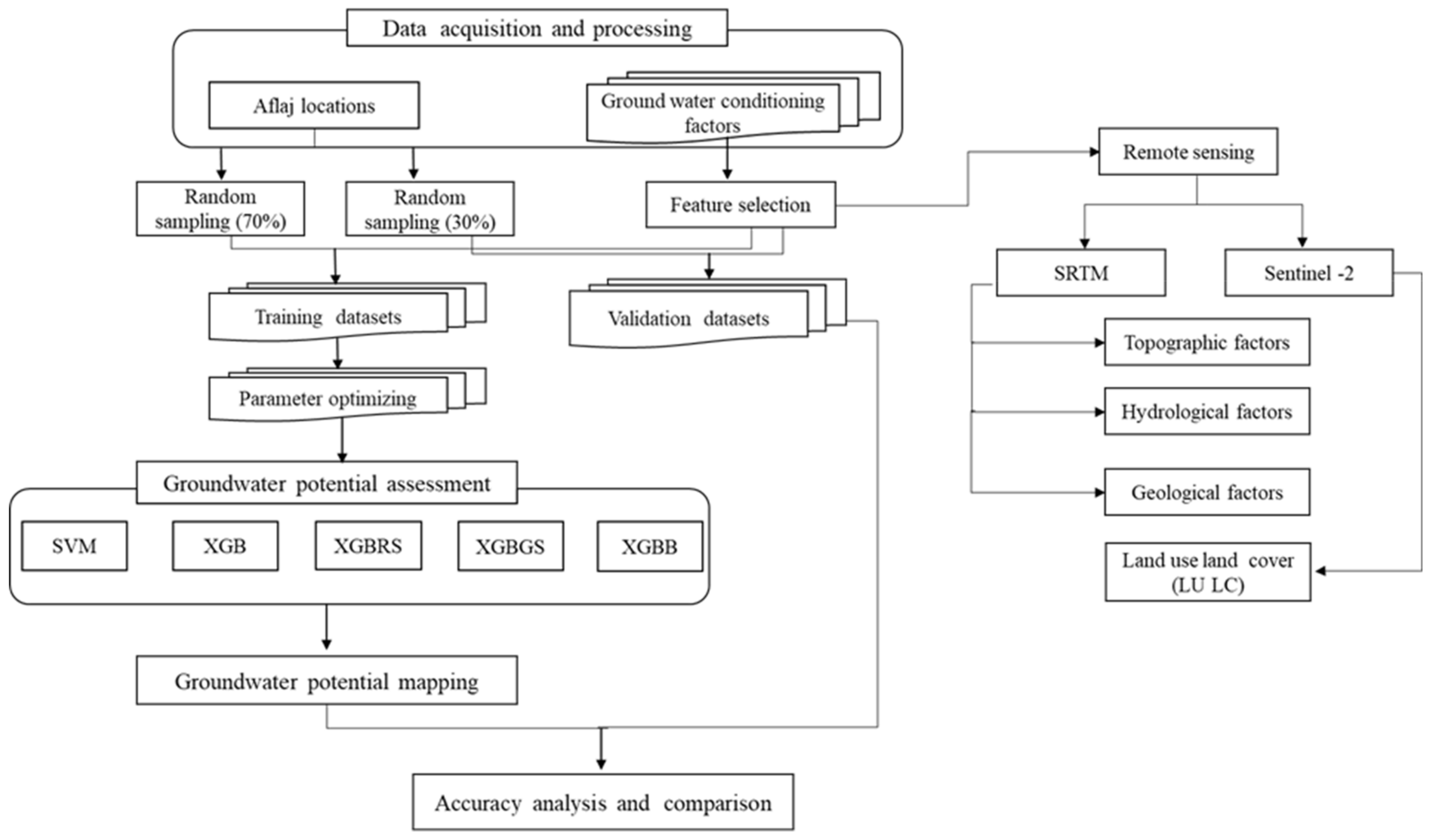
2. Materials and Methods

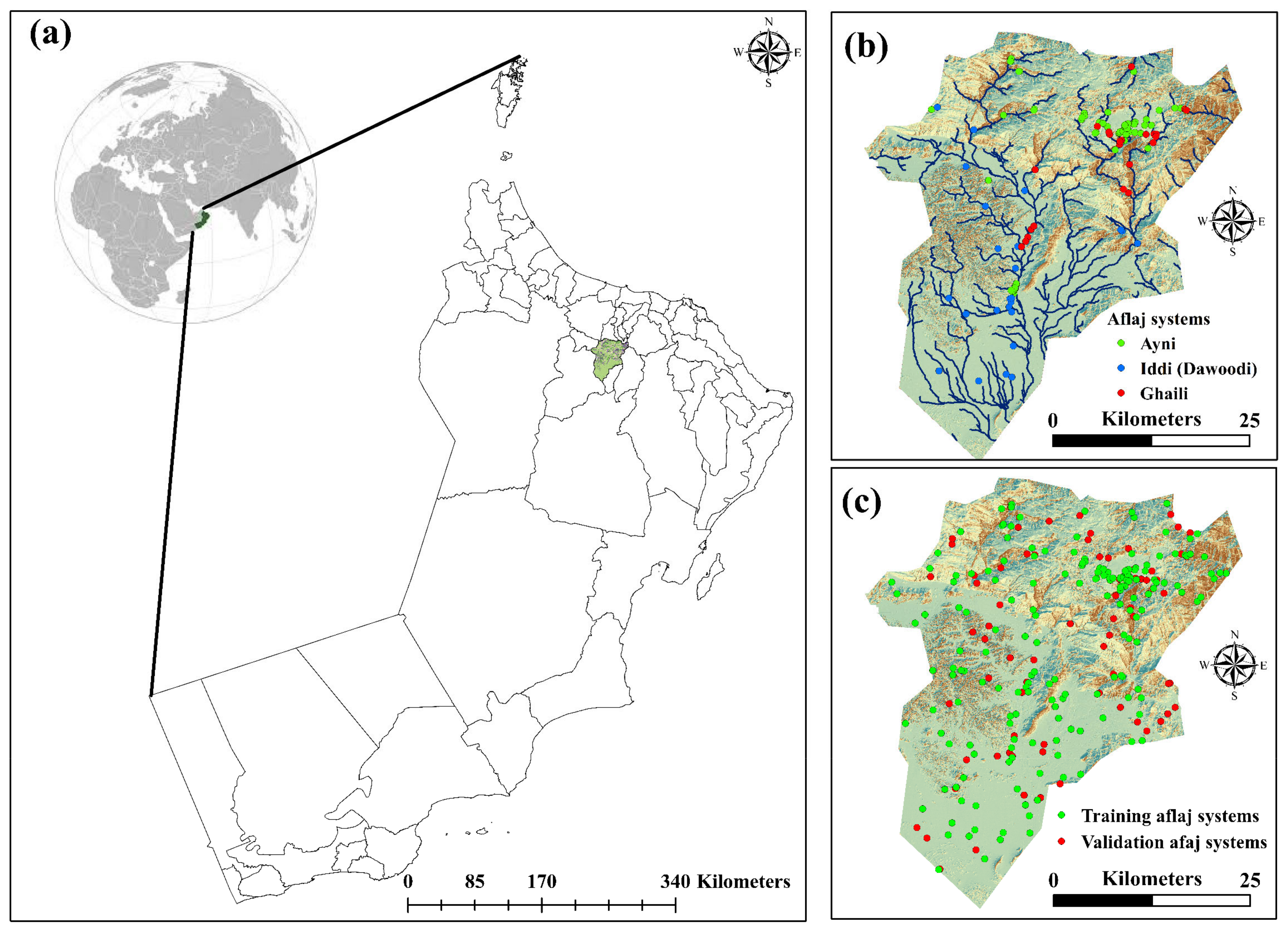
2.1. Study Area

The city of Nizwa is the regional centre of the Dakhiliyah governorate in the Sultanate of Oman. The city is a focal point of aflaj that underlies the historical relationship between ecology, economic dynamics, agricultural systems, and human settlements (Figure 1). It is located between 57°20′16E, 23°2′22N, and 57°48′21E, 23°5′22N. The study area’s elevation ranges from 388 to 2491 m above sea level. Nizwa is located at the foot of Al Jabal Al Akhdar to the south, surrounded by mountains, dry rivers (wadis), and orchards. Palm trees tower over the city. Nizwa has an arid climate, mild weather from November to March, and temperatures as low as 12 °C in January. The summers are hot and dry, with temperatures reaching up to 45 °C in July. In the city, there are 134 falajs and three types of aflaj systems.

2.2. Dataset Preparation for Spatial Modelling

2.2.1. Aflaj Data

To model the aflaj groundwater potential, aflaj and non-aflaj points were generated in ArcGIS 10.8 using random point extensions. Of the 336 points, 168 were aflaj points, and 168 were non-aflaj points. The datasets were divided into training (135 or 70%) and validation (101 or 30%) randomly. The groundwater observation aflaj data were obtained from the MAFWR, Oman (https://www.maf.gov.om, accessed on 1 March 2022 ). The aflaj location map for the study area in 2021 was prepared based on a 1:10,000 scale topographical map to create maps of potential aflaj for the study area. An extensive field survey confirmed.

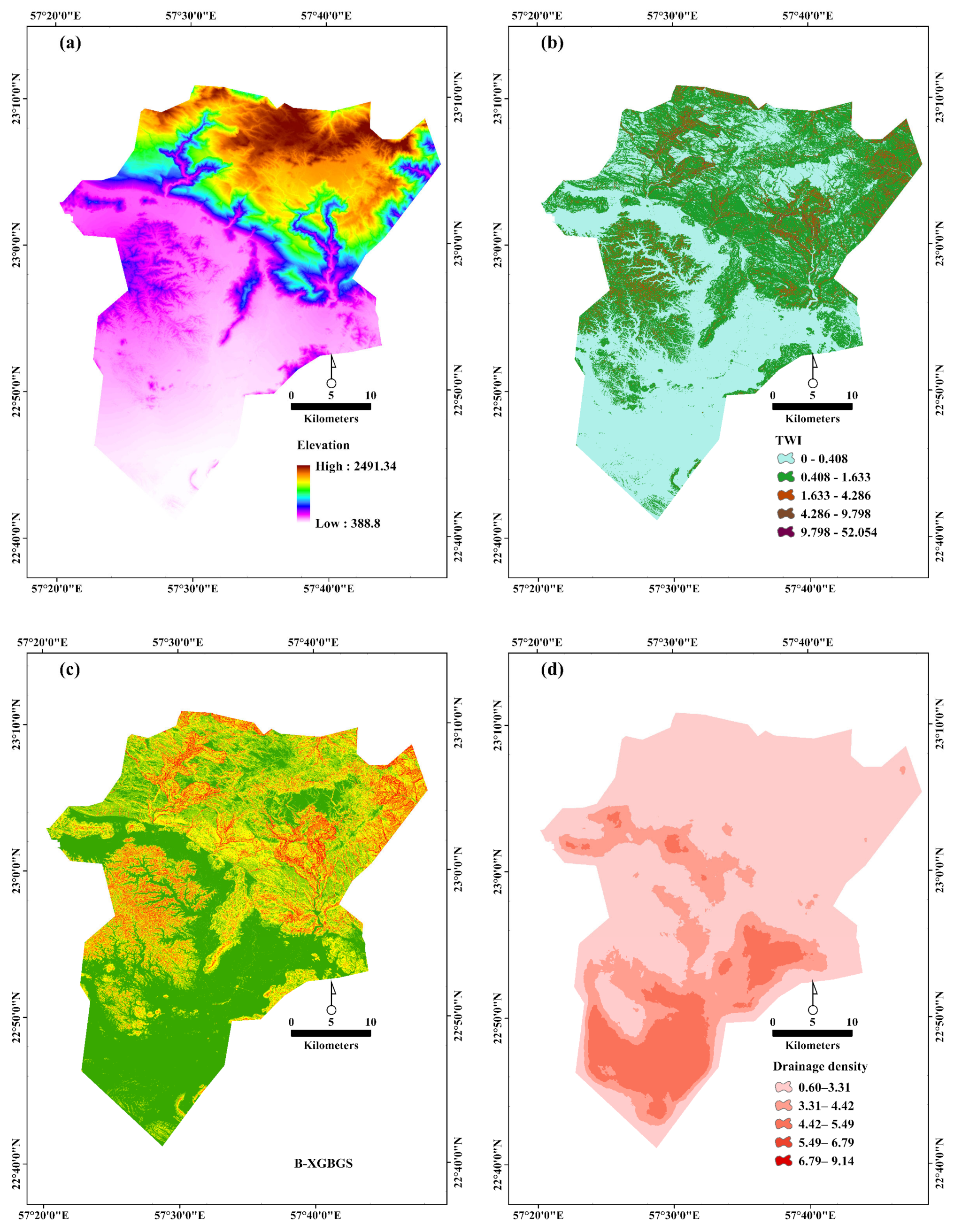
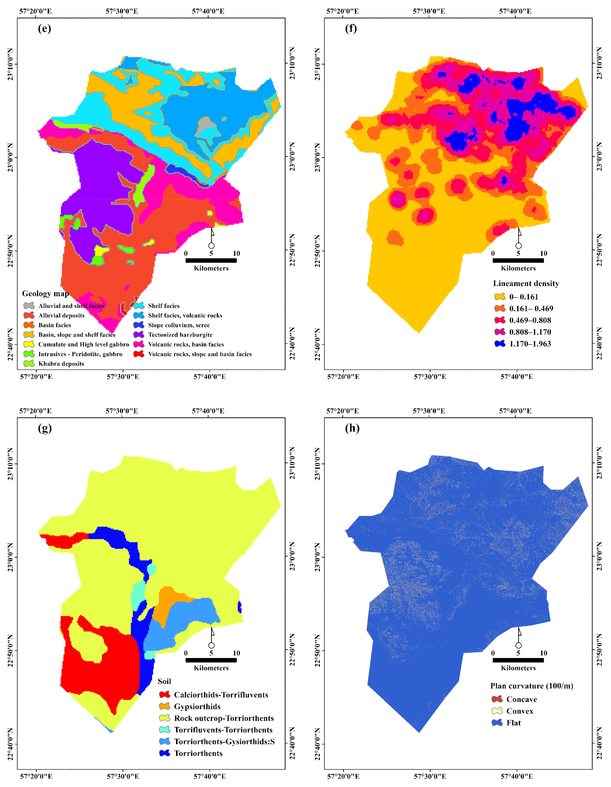
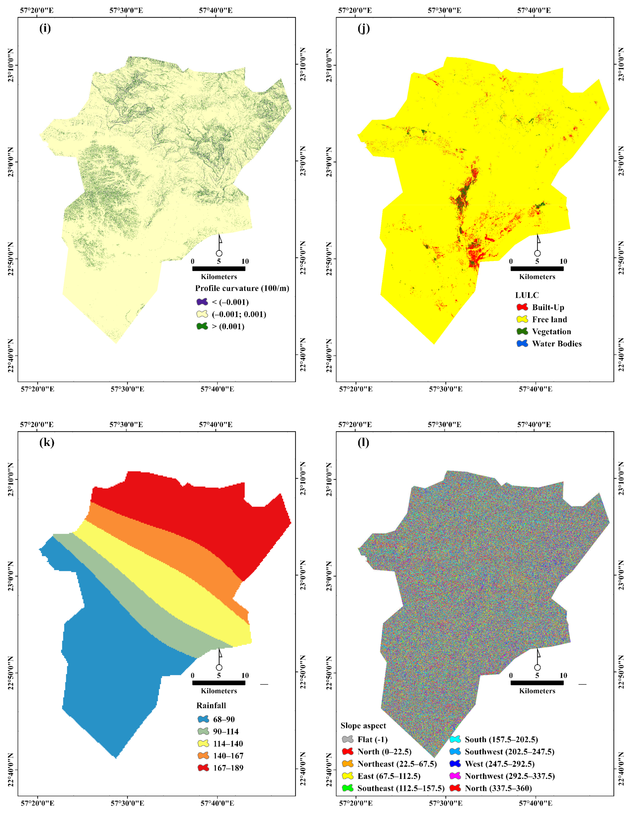
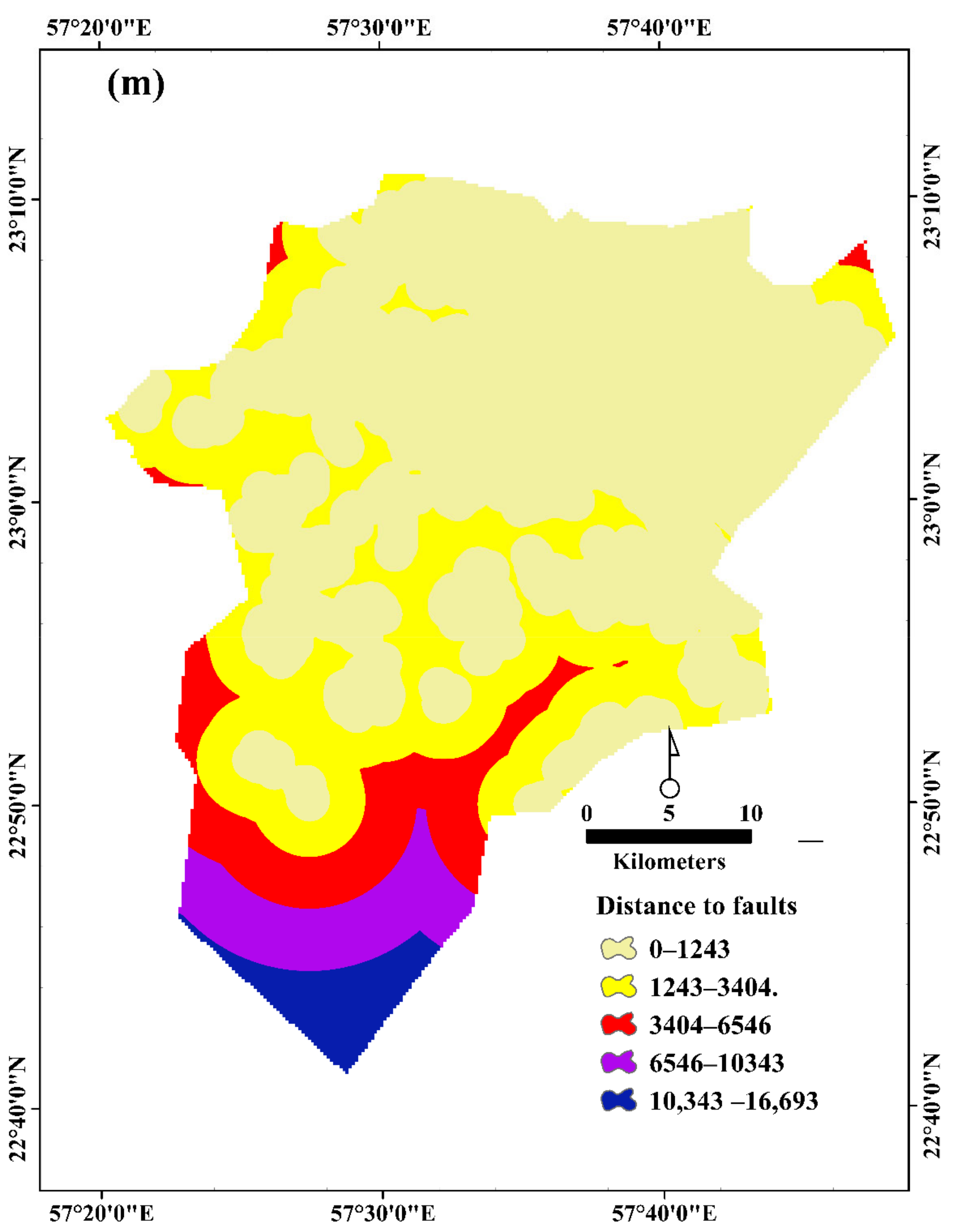
2.2.2. Groundwater Condition Variables

DEM: A DEM with a 5-metre two-dimensional resolution acquired from the National Survey Authority in Oman (http://nasom.org.om, accessed on 22 September 2020) was produced from light detection and ranging (LiDAR) data to derive thematic maps of groundwater condition variables. The main variables considered in this study, as well as those influencing the occurrence of aflaj, are discussed further below. This study evaluated thirteen significant aflaj variables: elevation, slope, slope aspect, TWI, geology, soil, plan curvature, profile curvature, drainage density, lineament density, LULC, distance to fault, and rainfall (Figure 2).

Topography: Topography is a geomorphologic factor used as a surface indicator to investigate groundwater potential. The elevation of the study area was calculated using a DEM with a resolution of 5 m and divided into five classes (Figure 2a). Changes in altitude can affect climate conditions, leading to changes in vegetation type, soil conditions, land use, and precipitation [32].

TWI: In the hydrogeological system, the TWI is critical (Figure 2b). It is widely used to describe how topographic impediments influence the location and size of saturated sources that generate surface runoff [33,34,35].

Slope: The slope of a physical characteristic is the degree of inclination of that surface to the horizontal and is a vital parameter for determining groundwater conditions. Zones with steep elevation angles have high runoff volumes and low infiltration rates. A watershed’s slope is one measure of the amount of water available for groundwater recharge and the terrain’s ruggedness. Slope influences runoff and infiltration rates. In this study, slope was determined in ArcGIS Desktop 10.8 using a DEM with a resolution of 5 m (Figure 2c). The study zone’s slope degree map was created and classified into five classes based on an equal interval scheme: 0–8, 8–21, 21–34, 34–51, and 51–88.

Drainage density: Drainage density indicates the closeness of the spacing of stream channels and can be calculated as the total length of all streams and rivers in the watersheds divided by the area of the drainage watershed. The drainage density has an inverse relationship with groundwater prospects. A zone with low-drainage- density causes more infiltration and decreased surface runoff and is suitable for groundwater development. Based on the surface-drainage density, the study area is grouped into five classes: 0.60–3.31, 0.31–4.42, 4.42–5.49, 5.49–6.79, and 6.79–9.14 km/km². Drainage density indirectly affects the groundwater potential of the study area; its values were calculated using the line density function in ArcGIS Pro 2.9 (Figure 2d).

Geological map: The geological map of the study area was classified into alluvial and self-facies, alluvial deposits, basin facies, basin slope and shelf facies, cumulate, and high-level gabbro, intrusive-peridotite and gabbro, khabra deposits, shelf facies, and volcanic rocks, slope colluvium and scree, tectonised harzburgite, volcanic rocks, basin facies, and slope (Figure 2e).

Lineament: The lineament viscosity map of the Nizwa watershed was assembled using line attributes obtained from the Geological Survey of Oman (http//www.pdo.co.om/, accessed on 1 July 2021) (Figure 2f).

Soil: The soil types in the study area play a critical role in aflaj groundwater potential and water-holding capacity; they are essential in delineating aflaj groundwater potential areas (Figure 2g). The soil groups found in the study area included rock outcrop, torriorthents, calciorthids-torrioifluvents-torriorthents, torrioifluvents-torriorthents, gypsiorthids (loamy), and torriorthents-gypsiorthids. The soil type was obtained from the MAFWR (https://www.maf.gov.om/, accessed on 22 July 2021).

Curvature: The curvature of a curve or the curvature of a surface deviates from that of a straight line or plane. Curvature is a topographical factor that depicts directional flow and specifies the rate at which the maximum slope direction changes. Positive curvature represents a convex area, zero curvature shows a flat area and negative curvature represents a concave area. The plan curvature map was created from the DEM using the surface analyst tool in ArcGIS Pro software (Figure 2h). Based on the standard classification, the profile curvature was determined and categorised into three groups, including <(−0.001), (−0.001; 0.001) and >(0.001) (Figure 2i).

Land-use/land cover: A supervised classification technique produced the land use map from the Sentinel-2 data. Sentinel is an earth satellite program designed, managed, and launched by the European Space Agency (ESA). Sentinel-2A and B are multispectral, high-resolution land observation satellites that capture images in thirteen bands and at multiple geometrical resolutions. This study used a free-cloud image and classified it into four major land use classes: vegetation, bare land, developed land, and water bodies. The accuracy of the land use classification was calculated as 94% using the Kappa index. Figure 2j presents the LULC map.

Rainfall: Rainfall data from 1975–2021 at two stations in the city were obtained from the Civil Aviation Authority, Oman (http://met.gov.om, accessed on 30 December 2021). The data were used to create a thematic map using geostatistical inverse distance weighted (IDW) interpolation in ArcGIS Pro 2.9. According to the IDW results, the annual precipitation ranged from 68 mm–190 mm in the study area. Rainfall is a critical parameter in determining aflaj groundwater potential and significant hydrologic sources of groundwater storage. Rainfall is typically heavier in the upper part of the study area, decreasing in the south (Figure 2k). Based on standard classifications, slope/aspect was divided into nine groups, indicating eight directions and flat zones (Figure 2l). The SVM, XGB, RS-XGB, GS-XGB, and XGBO models were applied to all aflaj factors using a raster grid. Finally, all leading aflaj factors were converted to a raster grid with 5 × 5 m cells. The flowchart illustrates the steps of data analyses in the study area. The materials and methods are given in the flowchart of Figure 3.

2.3. Multicollinearity Analysis

Correlation analysis of multicollinearity variance inflation factors (VIF) was used to evaluate the impact of each variable on the accuracy of the final aflaj maps. VIF determines whether two or more variables tell the same story [36]. According to the theory, any variable with a value greater than 7.5 should be eliminated from consideration. Multicollinearity testing using VIF was performed on a pool of 13 conditioning factors chosen to match the conceptual model as the first step in the ML analysis. The VIF values should all be less than the ESRI-defined threshold of 7.5, indicating that these variables are not redundant.

2.4. Machine Learning Methods

2.4.1. Support Vector Machine (SVM)

The SVM method is a well-known ML algorithm based on the Vapnik concept (1995). This technique is applied to study and control complex engineering systems. In terms of the structural risk minimisation norm, it can detect any interconnection between input and output variables. Based on the training dataset, this method determines the most practical combination of conditioning factors and applies these criteria to the entire dataset to predict possible groundwater locations [37]. As a result, SVM is more advanced and has a more complex structure than other statistical methods. Furthermore, even with a small training dataset, SVM is efficient.

The classification hyperplane was constructed at the centre of the maximum separation between the two classes by the SVM. If the point is above the hyperplane, it is assigned a value of +1; otherwise, it is assigned a value of −1 [38]. Support vectors are the training points closest to the optimal hyperplane [39]. This process begins with the training data of instance-label pairs (x_i, y_i) with x_i ϵRⁿ, y_iϵ(1, −1) and i = 1, …, m. x is a vector of input space that comprises the slope, elevation, slope aspect, TWI, rainfall, geology, soil types, fault density, drainage density, plain curvature, profile curvature, distance to faults, and LULC. The two values’ classes (1, −1) donate aflaj pixels and non-aflaj pixels. SVM proposes optimal hyperplane separation from the training set into aflaj and non-aflaj 1, −1 data.

2.4.2. Extreme Gradient Boosting (XGB)

XGB is an ML algorithm that uses a gradient-boosting structure, but with the added benefit of parallel tree boosting. It employs a more regularised algorithm than gradient boosting to combat overfitting, resulting in improved performance. To predict the output, XGB uses a boosting method that combines many weak learners [40] and parallel processes to reduce the total calculation time. The linear booster is useful in situations in which relationships are complex. Step-by-step information about XGB can be found in [41].

2.5. Hyperparameters Algorithm

2.5.1. Grid Search

Hyperparameter algorithms are configuration points that allow an ML model to be tailored to a specific task or dataset. Grid search (GS) experiments are commonly employed to optimise the hyperparameter of learning algorithms in empirical ML approaches [42]. Multistage, multi-resolution grid experiments that are more or less automated are commonly used because a grid experiment with a fine enough resolution for optimisation would be prohibitively expensive [43]. Aflaj potential was modelled using a GS with a set of fixed parameter values essential for optimal accuracy based on n-fold cross-validation. The optimal parameters, such as the number of characteristics to examine at each split, the maximum tree depth, the number of trees in the forest, and the minimum number of samples required to be split at the leaf node, were determined using the GS algorithm [44]. We used GS to investigate and model potential aflaj groundwater in the Nizwa watersheds.

2.5.2. Random Search

According to the literature, random search (RS) is more efficient than GS for hyperparameter optimisation in several ML algorithms on various datasets. In most cases, the RS found better models and required less computational time than the GS experiments of Larochelle, et al. [45]. For practical reasons related to the statistical independence of each trial, random experiments are easier to conduct than grid experiments. To obtain more accurate results in investigating, modelling, and mapping, RS was used to model the aflaj potential groundwater in the study area.

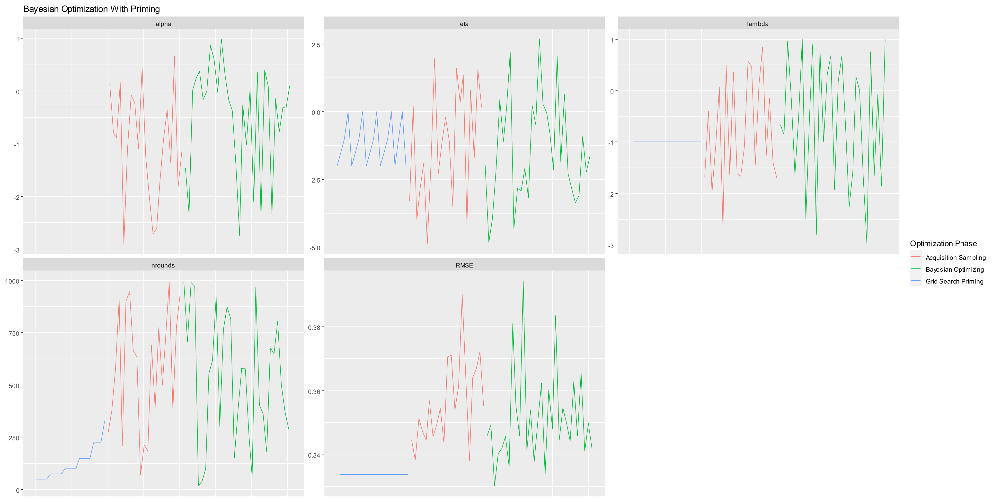
2.5.3. Bayesian Optimization (BO)

Bayesian optimisation (BO) is useful for finding the extrema of computationally expensive functions to solve. It can be used to solve tasks that lack a closed-form expression and functions that are difficult to calculate, have complex derivatives, or are non-convex. The theory of BO combines the prior distribution of the function f(x) with the sample evidence (information) to gain the posterior of the function, which is then used to identify where the function f(x) is maximised according to a characteristic. Although the Bayesian algorithm has been broadly used to prototype landslides [46,47], this study is the first to use the Bayesian algorithm to investigate and map aflaj groundwater potential in the Nizwa watershed. The BO method is derived from Bayes’ theorem, and proper step-by-step instructions can be found in [48].

2.6. Validation of Delineated Aflaj Groundwater Potential Zones

A common summary statistic to describe the receiver operating characteristics (ROC) curve is to calculate the area under the RCO carve. A measure with perfect predictive power would yield a value of 1.0, while one with no power would yield one of 0.5. Values less than 0.5 indicate a measure that is systematically incorrect. The maps of the aflaj groundwater potential zone were validated using data from existing aflaj systems. The aflaj data was prepared and overlaid on the study areas’ aflaj potential groundwater maps. ROC was used to determine the accuracy of aflaj potential groundwater zone maps. Python software was used to plot the validation results.

3. Results

3.1. Model Input Variables

A multicollinearity investigation was employed to determine suitable independent factors for modelling groundwater potential and included two criteria: VIF and tolerance. The results of the multicollinearity analysis of thirteen independent variables affecting groundwater potential are shown in

Table 1. The multicollinearity evaluation of thirteen independent variables.

Variables	VIF	Tolerance
Slope Aspect	1.19	0.84
Elevation	4.08	0.25
Drainage Density	2.59	0.39
Distance from fault	2.08	0.48
Geology	1.63	0.61
Lineament density	3.74	0.27
LULC	1.21	0.82
Plan curvature	1.34	0.74
Profile curvature	1.48	0.68
Annual rainfall	4.80	0.21
Slope	1.62	0.62
Soil	2.32	0.43
TWI	1.64	0.61

. The highest collinearity was related to the elevation variable, with a VIF of 4.08 and a tolerance of 0.25. All variables had a VIF of less than five, so no high collinearity was observed. Therefore, these thirteen independent variables were considered suitable for modelling groundwater potential in the Nizwa watershed.

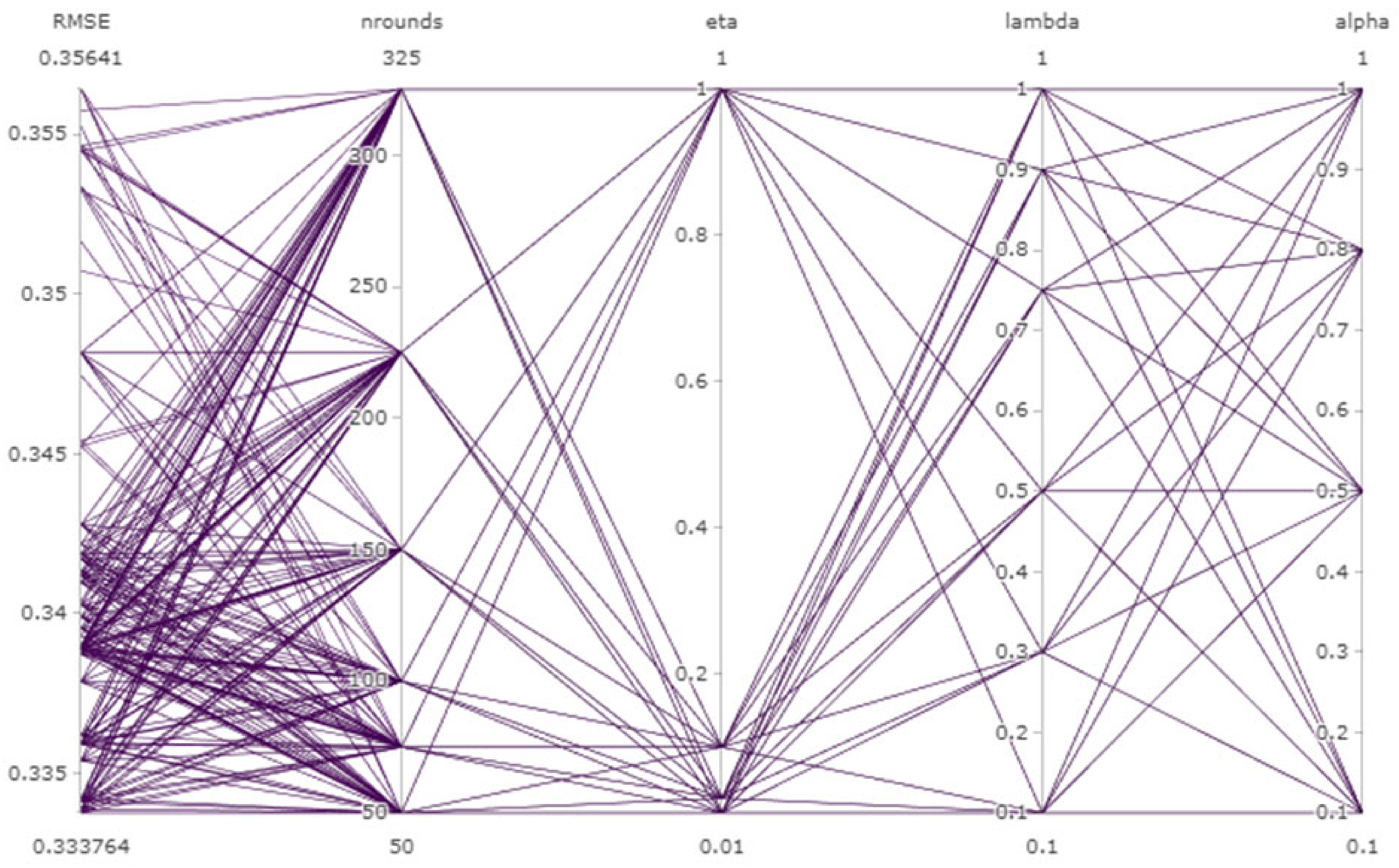
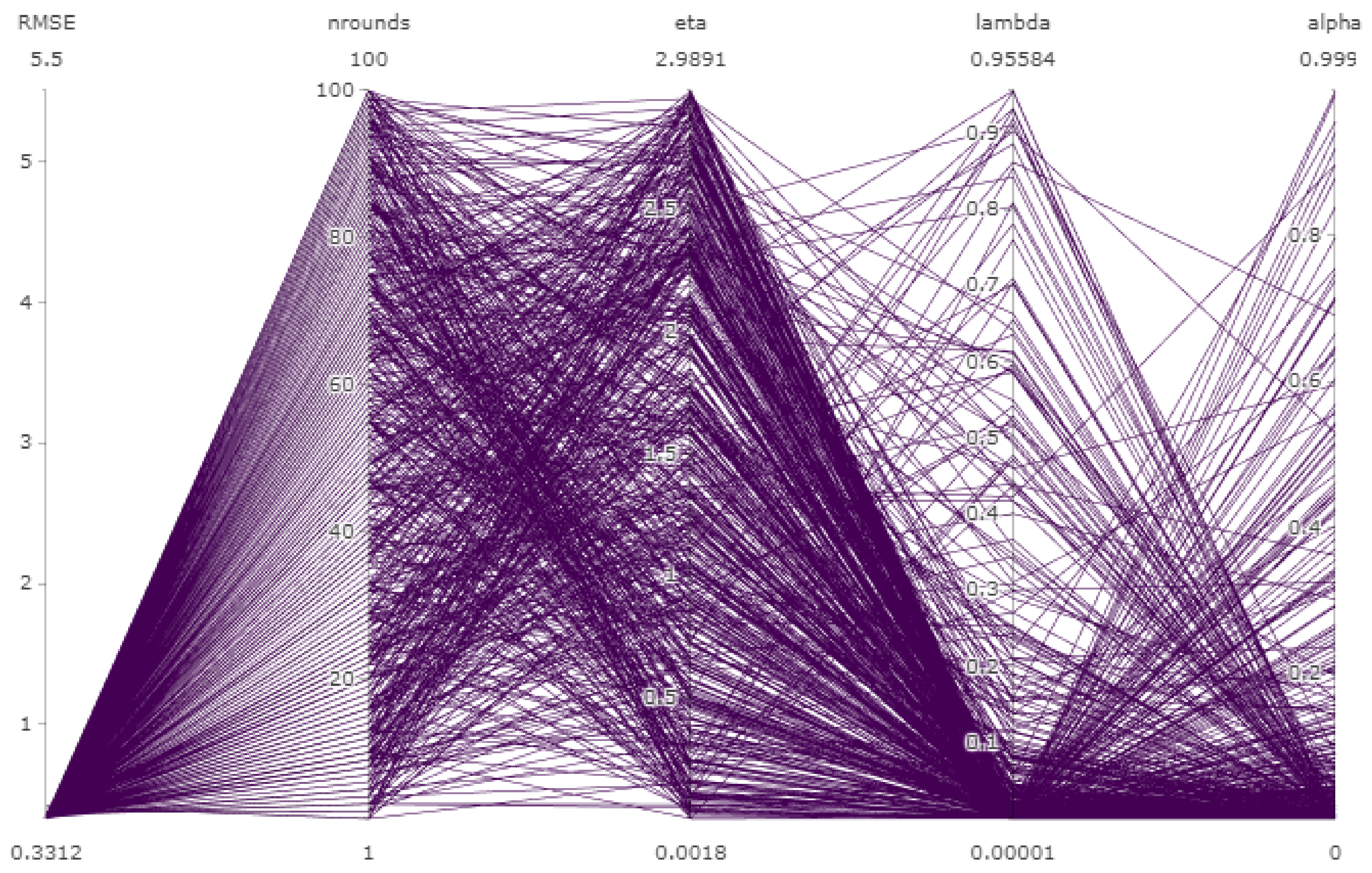
3.2. Hyperparametres of XGB Model Parameters

It is vital to calculate optimisation parameters for better modelling and efficient prediction. This study applied three hyperparameter algorithms—GS, RS, and BO—to optimise four XGB model parameters (nround, eta, lambda, and alpha) in aflaj groundwater potential. The optimisation results of the XGB model parameters based on GS, RS, and BO are shown in Figure 4, Figure 5 and Figure 6, respectively.

Table 2. Optimised parameters based on three hyperparameter algorithms.

	nround	lamba	alpha	eta	Error
XGB	30	0.5	1	0.1	0.345
GSXGB	50	0.3	1	0.1	0.3392
RSXGB	10	0.05472368	0.9992012	2.6803	0.3416736
BXGB	988	0.03476	1.060648	0.0001133161	0.322051

shows the optimal parameters for the XGB model, as determined by the GS, RS, and BO hyperparameter algorithms.

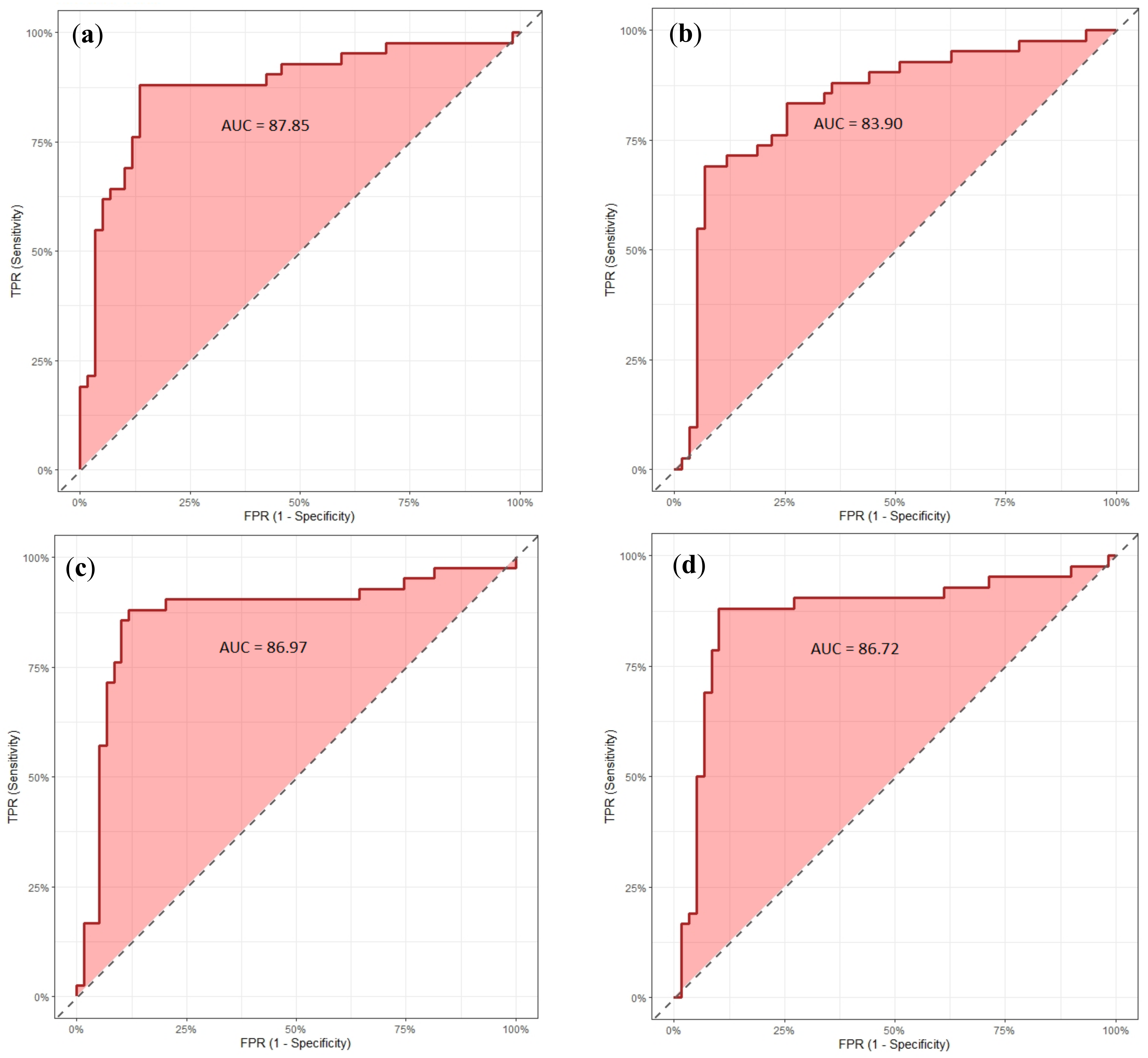
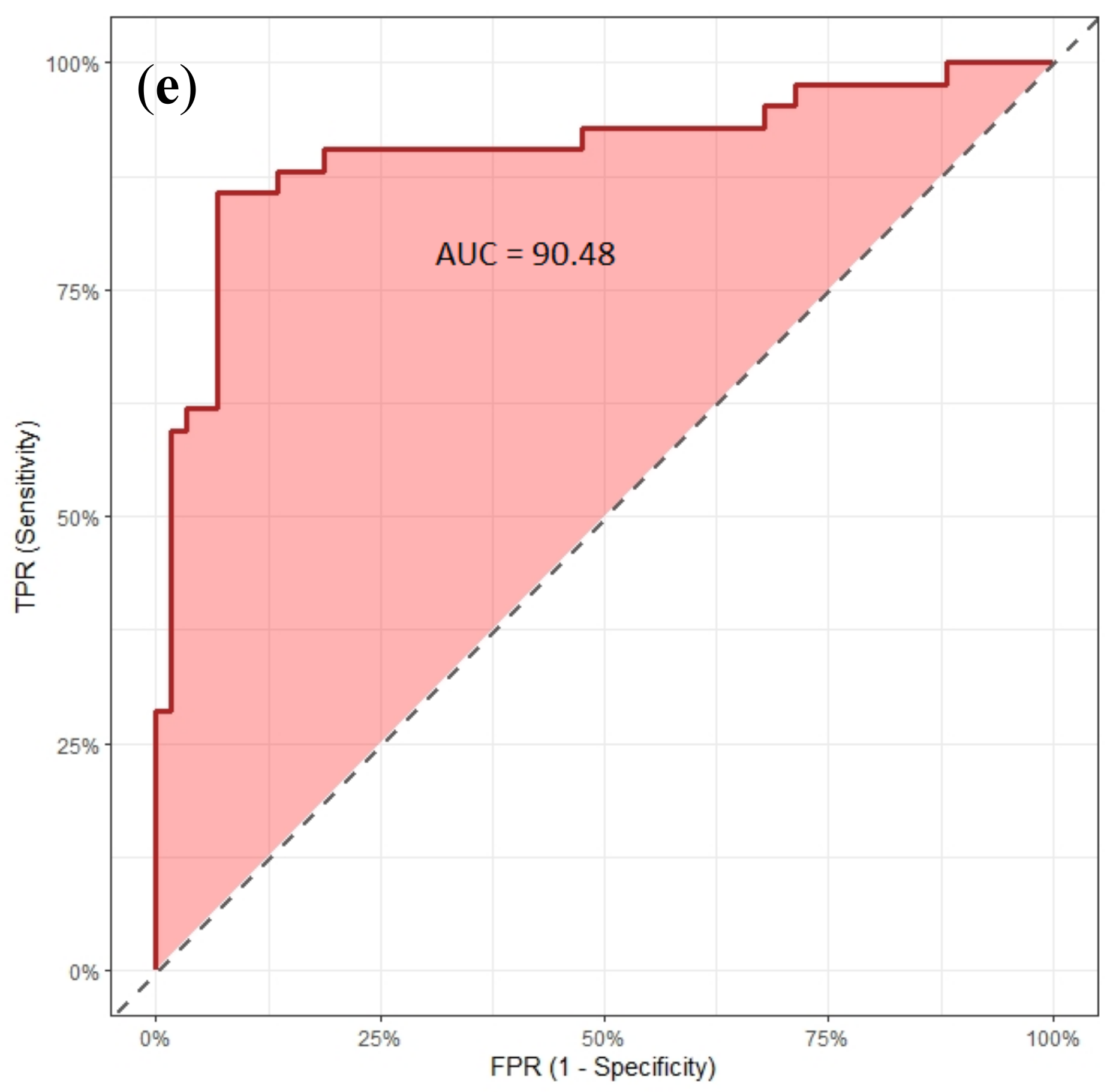
3.3. Model Validation

Validation of the ML models is a significant step in modelling groundwater potential. This investigation used five receivers operating characteristic (ROC) criteria to evaluate ML models in the training and validation stages. The results of the evaluation of five ML algorithms in modelling groundwater aflaj potential are shown in

Table 3. Model evaluation during the training and testing phases.

Models	Stage	Criteria
		Sensitivity	Specificity	PPV	NPV	AUC
	Train	0.87	0.86	0.88	0.85	0.96
SVM	Test	0.88	0.78	0.74	0.90	0.88
	Train	0.89	0.88	0.89	0.91	0.93
XGB	Test	0.76	0.75	0.68	0.81	0.84
	Train	0.89	0.91	0.91	0.93	0.97
GS-XGB	Test	0.86	0.88	0.83	0.89	0.87
	Train	0.89	0.88	0.89	0.91	0.96
RS-XGB	Test	0.88	0.88	0.84	0.91	0.87
	Train	0.96	0.97	0.97	0.98	0.99
Bayesian-XGB	Test	0.88	0.86	0.82	0.91	0.90

. A high level of accuracy was recorded for the Bayesian-XGB (0.99), GS-XGB (0.97), RS-XGB (0.96), SVM (0.96), and XGB (0.93) based on the AUC criteria (Figure 6). As shown in Figure 7 and Table 3, the three applied hyperparameter algorithms increased the efficiency of the XGB model in the training and validation stages. The validation showed that the Bayesian hyperparameter algorithm increased the XGB’s efficiency in modelling groundwater aflaj potential. The evaluation of efficiency for the five ML algorithms based on AUC criteria in the validation stage showed high efficiency for the Bayesian-XGB (90.48%), SVM (87.85%), GS-XGB (86.97%), RS-XGB (86.72%), and XGB (83.90%).

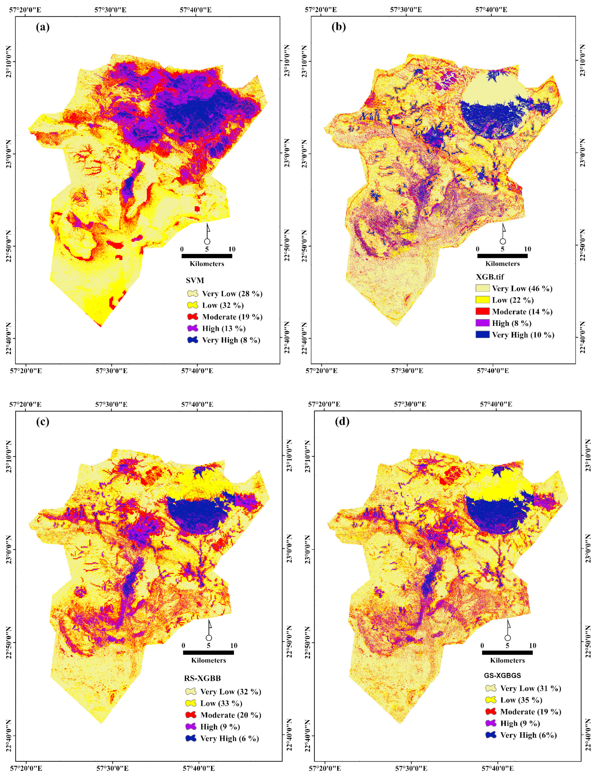
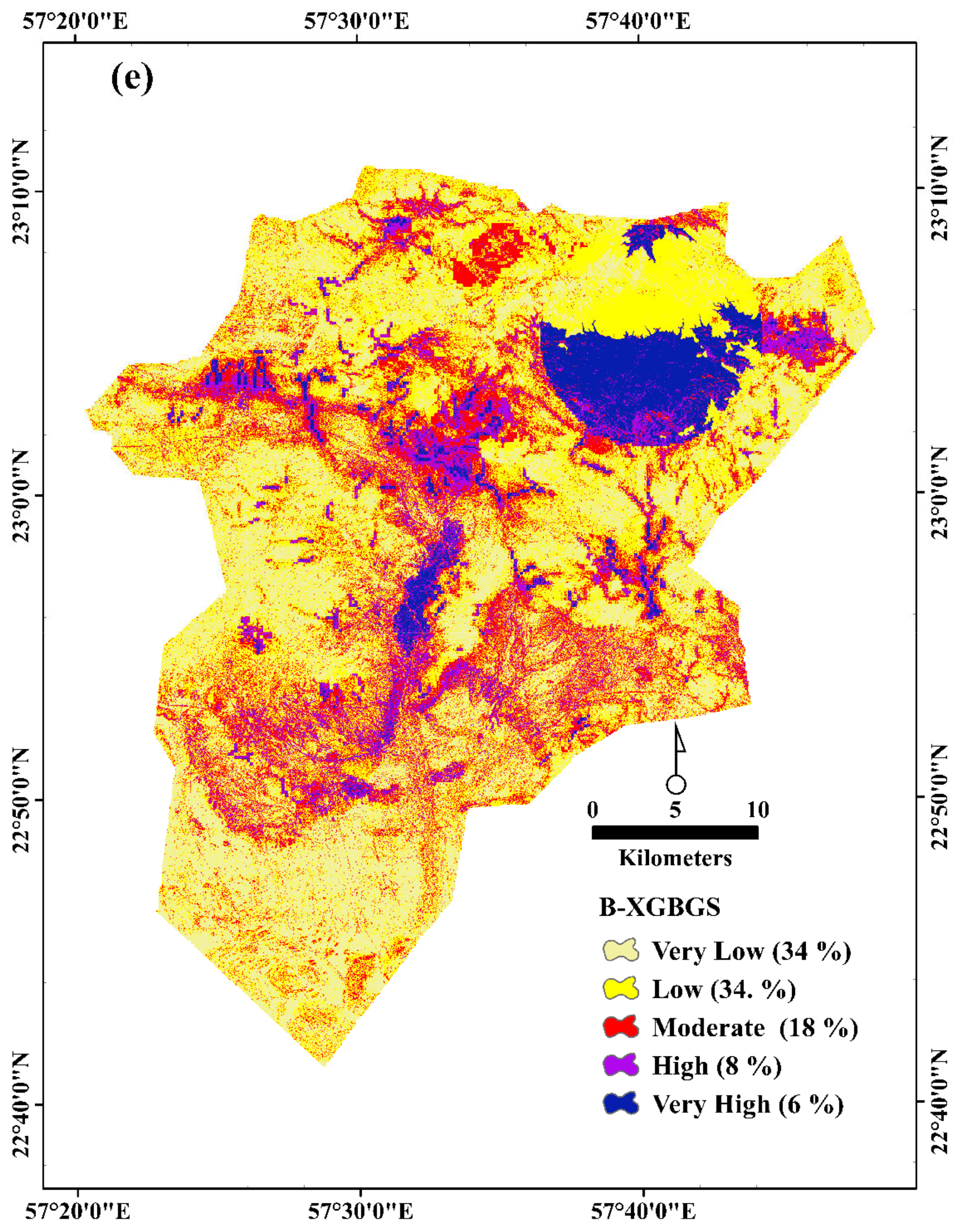
3.4. Groundwater Potential Mapping

Groundwater aflaj potential maps were predicted based on five ML algorithms: SVM, XGB, GS-XGB, RS-XGB, and Bayesian-XGB. The groundwater potential was envisioned as a probability between 0 and 1. This probability was reclassified to represent the groundwater potential classes into very low, low, moderate, high, and very high, based on the natural break method in ArcGIS 10.7. The maps of groundwater potential and the percentage of each class are shown in Figure 8. The highest rate of groundwater potential was very high in the XGB (10%), SVM (8%), GS-XGB (6%), RS-XGB (6%), and Bayesian-XGB (6%) models. Most of these areas were located in the central and northeastern portions of the study area.

3.5. Importance Value

The results of the variables’ importance in aflaj groundwater potential modelling based on the five ML algorithms are shown in

Table 4. Importance value.

Variables	SVM	XGB	GS-XGB	RS-XGB	B-XGB
Annual rainfall	84.75	100.00	100.00	100.00	100.00
Slope Aspect	9.54	21.82	9.86	9.57	9.30
Distance from fault	76.15	29.44	26.81	26.68	25.05
Drainage density	45.87	18.74	8.37	8.10	8.38
Elevation	97.31	48.97	40.02	39.38	40.41
Geology	5.19	2.03	10.23	10.17	8.03
Lineament density	100.00	4.69	9.45	9.25	10.64
LULC	0.43	0.09	3.13	3.10	0.46
Plan curvature	10.36	14.38	8.17	7.00	4.65
Profile curvature	26.45	8.92	6.34	5.43	3.04
Slope	23.11	33.57	20.90	20.64	23.79
Soil	2.42	0.02	0.03	0.01	0.02
TWI	14.89	5.99	5.05	4.07	2.19

. The thirteen variables that affected aflaj groundwater potential had different effects on groundwater potential modelling in the case study. In the SVM model, lineament density, elevation, annual rainfall, and distance from the fault had the highest importance, while LULC, soil, and geology had the lowest importance. In the XGB, GS-XGB, RS-XGB, and B-XGB models, annual rainfall, elevation, and distance from fault variables, respectively, made substantial contributions to groundwater potential modelling. At the same time, soil, LULC, and geology, respectively, made weak contributions.

4. Discussion

In recent years, climate change and improper groundwater use have led to the spatial modelling of groundwater potential. Researchers have emphasised the importance of understanding the factors that better forecast groundwater resources in arid and semi-arid regions, where groundwater plays a vital role in the water supply for various services. Generally, spatial modelling of natural phenomena is complex, and no algorithm can make perfect or complete predictions [49]. Therefore, researchers use contradictory algorithms and methods to predict and model with appropriate accuracy. This study used SVM and XGB ML models to predict groundwater potential in the Nizwa watershed. The study used three hyperparameter algorithms (GS, RS, and BO) to optimise the parameters of the XGB model.

The variables of slope, slope aspect, attitude, profile curvature, plan curvature, TWI, drainage density, lineament density, and LULC were used to map the aflaj groundwater potential in the study area. The multicollinearity evaluation of thirteen independent variables showed that all variables had a VIF of less than five, so no high collinearity was observed. Therefore, these thirteen independent variables were considered suitable for modelling groundwater potential in the Nizwa watershed (Table 1).

The study results revealed that the three algorithms used in optimising the parameters of the XGB model enhanced the productivity of the XGB model in modelling the aflaj groundwater potential in the study area (Figure 4, Figure 5, Figure 6 and Figure 7). Tuning the ML parameters based on hyperparameter algorithms increased the model’s efficiency [50,51]. Various scholars [52,53] in the field of natural hazard modelling have used hyperparameter algorithms, such as RS and GS, to determine the optimal parameters of ML models; their results have shown that these algorithms have a positive effect on improving model performance. For groundwater potential modelling, Al-Fugara, Ahmadlou, Al-Shabeeb, AlAyyash, Al-Amoush, and Al-Adamat [54] determined the optimal parameters in the SVR model using hyperparameter RS and genetic algorithms. Their findings demonstrated that these algorithms improved the SVR model’s performance in groundwater potential modelling.

The effect of hyperparameter algorithms on the performance of the XGB model in groundwater aflaj potential modelling in the Nizwa watershed showed that the Bayesian-XGB algorithm had better performance than the RS-XGB and GS-XGB algorithms (Table 2 and Figure 7). By increasing the number of samples and input/output data, the Bayesian algorithm adjusted the objective function’s posterior distribution to optimise the model parameter and obtain the best parameters [55,56]. The high efficiency of using BO for optimising ML algorithms, such as random forest, logistic regression, and SVM models, has been confirmed in landslide hazard modelling [57,58]. Janizadeh, et al. [59] also used BO to optimise XGB model parameters to model flood susceptibility. Their results showed that the Bayesian hyperparameter algorithm enhanced the performance of the XGB model in modelling flood susceptibility.

This study highlighted the relative importance of the 13 independent variables in groundwater aflaj potential modelling, but demonstrated that annual rainfall, elevation, and distance from fault variables are more important than other variables in modelling (Table 3). The mountainous zone of the study area has the highest aflaj groundwater potential. All five maps displayed very high aflaj groundwater potential in the study area (Figure 8) because of the numerous faults that cause water to pool between the faults, resulting in the formation of wet fractures and the installation of water resources in the alluvium. Abrams, et al. [60] observed that moisture fissures support the use of lineament density to represent the fracture systems’ role as groundwater conduits in the western Hajar Mountains of Oman. The aflaj collect and discharge the water from these moisture fissures. As a result, high lineament densities increase the ability to store and transmit groundwater via the secondary porosity of fractures in the subsurface. Negative curvatures also indicate areas where runoff may pool or channel, potentially increasing infiltration.

Although standing water at the valley bottoms can indicate a saturated subsurface or poor infiltration conditions, the presence of water resources in alluvial deposits suggests enough groundwater for human use in this area. Our findings showed that the lowest (very low) aflaj groundwater potentials were located away from the mountain plains. The average annual rainfall in most parts of the country is less than 100 mm, but it can reach 350 mm in mountainous areas. The geology and hydrogeology of Oman are complex, and there are many different aquifer systems, many of which are relevant only in local areas.

This research suggests that ML algorithms are adequate for aflaj system groundwater prospecting and that using remote sensing-derived variables and advanced GIS layers improves the model accuracy and precision of aflaj groundwater potential maps. Even if a given study area contains many variables that influence hydrogeological conditions, most can be precisely mapped using ML, deep learning methods, remote sensing, and GIS products. This is especially important for large study areas like remote or undeveloped regions and data-scarce locations where ground-based investigations like geophysical and direct hydrological surveys are impractical. Both surface and subsurface geology and lineaments must be carefully considered during aflaj groundwater potential indexing.

To index groundwater potential in varying layers, knowledge-based approaches are necessary. The effectiveness of the SVM and XGB ML models, as well as the hyperparameter algorithms GS, RS, and BO to optimise the parameters of the XGB maps, supports the use of knowledge-based techniques for calculating semi-quantitative models of aflaj groundwater potential, enabling extrapolation of aflaj groundwater potential in areas with a shortage of data.

5. Conclusions

SVM and XGB ML models were used in this study to model and predict groundwater potential in the Nizwa watershed. The primary goal of this study was to optimise the parameters of the XGB model using three hyperparameter algorithms: GS, RS, and BO. The variables of slope, aspect, attitude, plan curvature, profile curvature, TWI, drainage density, and lineament density were calculated using LiDAR data and GIS. Sentinel-2 satellite data were used to map the LULC. Based on the evaluation of accuracy in the training stage, the following models showed a high level of accuracy based on the AUC: Bayesian-XGB (0.99), GS-XGB (0.97), RS-XGB (0.96), SVM (0.96), and XGB (0.93). The ML and hyperparameter algorithms’ factor analysis results recommended thirteen factors to investigate and map aflaj groundwater potential in the study area. Thus, the study concluded that evaluating existing groundwater datasets, facilities, and current and future spatial datasets is critical for designing systems capable of mapping groundwater aflaj based on geospatial and ML techniques. In turn, groundwater protection service projects and integrated water source management (IWSM) programs will be able to safeguard the aflaj irrigation system by implementing timely preventative measures. The mapping of groundwater aflaj potential can contribute to the development of more effective management techniques for their control. In addition, mapping is necessary for developing predictive models that offer information on the likelihood of occurrence, spatial distribution, and density under various environmental variables. These updated maps will aid IWSM initiatives in educating and empowering authorities and organizations concerned with groundwater quality and quantity. Spatial modelling will also help reduce costs, like GIS, ML, and remote sensing-based methods developed to pursue this research promise more practical and cost-effective solutions. In addition, this research will save money on monitoring since the remote sensing-based technologies developed in this project will give a more efficient and cost-effective way to monitor water resources on a broad scale in Oman.

References

1. Chakkaravarthy, S.S.; Sangeetha, D.; Vaidehi, V. A survey on malware analysis and mitigation techniques. J. Comput. Sci. Rev. 2019, 32, 1–23. [Google Scholar] [CrossRef]
2. He, X.; Li, P.; Ji, Y.; Wang, Y.; Su, Z.; Elumalai, V. Groundwater arsenic and fluoride and associated arsenicosis and fluorosis in China: Occurrence, distribution and management. Expo. Health 2020, 12, 355–368. [Google Scholar] [CrossRef]
3. Döll, P.; Fiedler, K. Global-scale modeling of groundwater recharge. Hydrol. Earth Syst. Sci. 2008, 12, 863–885. [Google Scholar] [CrossRef] [Green Version]
4. Al-Marshoudi, A.S. Water institutional arrangements of FalajAl Daris in the sultanate of Oman. Int. J. Soc. Sci. Manag. 2018, 5, 31–42. [Google Scholar] [CrossRef] [Green Version]
5. Al-Ghafri, A. Overview about the Aflaj of Oman. In Proceedings of the International Symposium of Khattaras and Aflaj, Erachidiya, Morocco, 9 October 2018; pp. 1–22. [Google Scholar]
6. Alsharhan, A.S.; Rizk, Z.E. Aflaj systems: History and factors affecting recharge and discharge. In Water Resources and Integrated Management of the United Arab Emirates; Springer: Berlin/Heidelberg, Germany, 2020; pp. 257–280. [Google Scholar]
7. Rafik, A.; Bahir, M.; Beljadid, A.; Ouazar, D.; Chehbouni, A.; Dhiba, D.; Ouhamdouch, S. Surface and groundwater characteristics within a semi-arid environment using hydrochemical and remote sensing techniques. Water 2021, 13, 277. [Google Scholar] [CrossRef]
8. Fabro, A.Y.R.; Ávila, J.G.P.; Alberich, M.V.E.; Sansores, S.A.C.; Camargo-Valero, M.A. Spatial distribution of nitrate health risk associated with groundwater use as drinking water in Merida, Mexico. Appl. Geogr. 2015, 65, 49–57. [Google Scholar] [CrossRef]
9. Zomlot, Z.; Verbeiren, B.; Huysmans, M.; Batelaan, O. Spatial distribution of groundwater recharge and base flow: Assessment of controlling factors. J. Hydrol. Reg. Stud. 2015, 4, 349–368. [Google Scholar] [CrossRef] [Green Version]
10. Callegary, J.; Kikuchi, C.; Koch, J.C.; Lilly, M.; Leake, S. Groundwater in Alaska (USA). Hydrogeol. J. 2013, 21, 25–39. [Google Scholar] [CrossRef]
11. Sreedevi, P.; Subrahmanyam, K.; Ahmed, S. The significance of morphometric analysis for obtaining groundwater potential zones in a structurally controlled terrain. Environ. Geol. 2005, 47, 412–420. [Google Scholar] [CrossRef]
12. Forootan, E.; Seyedi, F. GIS-based multi-criteria decision making and entropy approaches for groundwater potential zones delineation. Earth Sci. Inform. 2021, 14, 333–347. [Google Scholar] [CrossRef]
13. Abdulkareem, J.; Pradhan, B.; Sulaiman, W.; Jamil, N.J.G.F. Prediction of spatial soil loss impacted by long-term land-use/land-cover change in a tropical watershed. Geosci. Front. 2019, 10, 389–403. [Google Scholar] [CrossRef]
14. Siswanto, S.Y.; Francés, F.J.E.E.S. How land use/land cover changes can affect water, flooding and sedimentation in a tropical watershed: A case study using distributed modeling in the Upper Citarum watershed, Indonesia. Environ. Earth Sci. 2019, 78, 1–15. [Google Scholar] [CrossRef]
15. Dibaba, W.T.; Demissie, T.A.; Miegel, K.J.W. Watershed hydrological response to combined land use/land cover and climate change in highland Ethiopia: Finchaa catchment. Water 2020, 12, 1801. [Google Scholar] [CrossRef]
16. Chen, W.; Li, H.; Hou, E.; Wang, S.; Wang, G.; Panahi, M.; Li, T.; Peng, T.; Guo, C.; Niu, C. GIS-based groundwater potential analysis using novel ensemble weights-of-evidence with logistic regression and functional tree models. Sci. Total Environ. 2018, 634, 853–867. [Google Scholar] [CrossRef] [PubMed] [Green Version]
17. Manap, M.A.; Nampak, H.; Pradhan, B.; Lee, S.; Sulaiman, W.N.A.; Ramli, M.F. Application of probabilistic-based frequency ratio model in groundwater potential mapping using remote sensing data and GIS. Arab. J. Geosci. 2014, 7, 711–724. [Google Scholar] [CrossRef]
18. Tahmassebipoor, N.; Rahmati, O.; Noormohamadi, F.; Lee, S. Spatial analysis of groundwater potential using weights-of-evidence and evidential belief function models and remote sensing. Arab. J. Geosci. 2016, 9, 1–18. [Google Scholar] [CrossRef]
19. Khoshtinat, S.; Aminnejad, B.; Hassanzadeh, Y.; Ahmadi, H. Application of GIS-based models of weights of evidence, weighting factor, and statistical index in spatial modeling of groundwater. J. Hydroinformatics 2019, 21, 745–760. [Google Scholar] [CrossRef]
20. Hou, E.; Wang, J.; Chen, W. A comparative study on groundwater spring potential analysis based on statistical index, index of entropy and certainty factors models. Geocarto Int. 2018, 33, 754–769. [Google Scholar] [CrossRef]
21. Kalantar, B.; Al-Najjar, H.A.; Pradhan, B.; Saeidi, V.; Halin, A.A.; Ueda, N.; Naghibi, S.A. Optimized conditioning factors using machine learning techniques for groundwater potential mapping. Water 2019, 11, 1909. [Google Scholar] [CrossRef] [Green Version]
22. Yariyan, P.; Avand, M.; Omidvar, E.; Pham, Q.B.; Linh, N.T.T.; Tiefenbacher, J.P. Optimization of statistical and machine learning hybrid models for groundwater potential mapping. Geocarto Int. 2020, 37, 3877–3911. [Google Scholar] [CrossRef]
23. Moghaddam, D.D.; Rahmati, O.; Panahi, M.; Tiefenbacher, J.; Darabi, H.; Haghizadeh, A.; Haghighi, A.T.; Nalivan, O.A.; Bui, D.T. The effect of sample size on different machine learning models for groundwater potential mapping in mountain bedrock aquifers. Cantena 2020, 187, 104421. [Google Scholar] [CrossRef]
24. Fadhillah, M.F.; Lee, S.; Lee, C.-W.; Park, Y.-C. Application of support vector regression and metaheuristic optimization algorithms for groundwater potential mapping in Gangneung-si, South Korea. Remote Sens. 2021, 13, 1196. [Google Scholar] [CrossRef]
25. Jamrah, A.; Al-Futaisi, A.; Rajmohan, N.; Al-Yaroubi, S. Assessment of groundwater vulnerability in the coastal region of Oman using DRASTIC index method in GIS environment. Environ. Monit Assess 2008, 147, 125–138. [Google Scholar] [CrossRef] [PubMed]
26. Elmahdy, S.; Ali, T.; Mohamed, M. Regional mapping of groundwater potential in ar rub al khali, arabian peninsula using the classification and regression trees model. Remote Sens. 2021, 13, 2300. [Google Scholar] [CrossRef]
27. Akhtar, J.; Sana, A.; Tauseef, S.M.; Chellaiah, G.; Kaliyaperumal, P.; Sarkar, H.; Ayyamperumal, R. Evaluating the groundwater potential of Wadi Al-Jizi, Sultanate of Oman, by integrating remote sensing and GIS techniques. Environ. Sci. Pollut. Res. 2022, 29, 1–12. [Google Scholar] [CrossRef] [PubMed]
28. Al-Ajmi, H.A.; Ahmed, M.; Rahman, H.A.A.; Al-Rawahy, S.A. Integrated Catchment Management in Arid Countries A Case Study: Wadi Al-Ayn Catchment, Northern Oman. Pak. J. Soc. Sci. 2005, 3, 242–249. [Google Scholar]
29. Al-Kalbani, M.S.; Price, M.F.; Ahmed, M.; Abahussain, A.; O’Higgins, T.; Argyll, U. Water quality assessment of Aflaj in the Mountains of Oman. Environ. Nat. Resour. Res. 2016, 6, 99. [Google Scholar] [CrossRef] [Green Version]
30. Al-Ghafri, A.; Inoue, T.; Nagasawa, T. Daudi aflaj: The qanats of Oman. In Proceedings of the Third Symposium on Xinjang Uyghur, China, Chiba, Japan, 11 November 2003. [Google Scholar]
31. Remmington, G. Transforming tradition: The aflaj and changing role of traditional knowledge systems for collective water management. J. Arid. Environ. 2018, 151, 134–140. [Google Scholar] [CrossRef]
32. Al-Kalbani, M.S.; Price, M.F.; O’Higgins, T.; Ahmed, M.; Abahussain, A.J.R.E.C. Integrated environmental assessment to explore water resources management in Al Jabal Al Akhdar, Sultanate of Oman. Reg. Environ. Chang. 2016, 16, 1345–1361. [Google Scholar] [CrossRef]
33. McCann, I.; Al-Ghafri, A.; Al-Lawati, I.; Shayya, W. Aflaj: The challenge of preserving the past and adapting to the future. In Proceedings of the Oman International Conference on the Development and Management of Water Conveyance Systems (Aflaj), Muscat, Oman, May 2002; pp. 18–20. [Google Scholar]
34. Nampak, H.; Pradhan, B.; Abd Manap, M. Application of GIS based data driven evidential belief function model to predict groundwater potential zonation. J. Hydrol. 2014, 513, 283–300. [Google Scholar] [CrossRef]
35. Pourghasemi, H.R.; Beheshtirad, M. Assessment of a data-driven evidential belief function model and GIS for groundwater potential mapping in the Koohrang Watershed, Iran. Geocarto Int. 2015, 30, 662–685. [Google Scholar] [CrossRef]
36. Pham, B.T.; Jaafari, A.; Prakash, I.; Singh, S.K.; Quoc, N.K.; Bui, D.T. Hybrid computational intelligence models for groundwater potential mapping. Catena 2019, 182, 104101. [Google Scholar] [CrossRef]
37. Arulbalaji, P.; Padmalal, D.; Sreelash, K. GIS and AHP techniques based delineation of groundwater potential zones: A case study from southern Western Ghats, India. Sci. Rep. 2019, 9, 1–17. [Google Scholar] [CrossRef] [Green Version]
38. Marcoulides, K.M.; Raykov, T. Evaluation of variance inflation factors in regression models using latent variable modeling methods. Educ. Psychol. Meas. 2019, 79, 874–882. [Google Scholar] [CrossRef] [PubMed]
39. Arabgol, R.; Sartaj, M.; Asghari, K. Predicting nitrate concentration and its spatial distribution in groundwater resources using support vector machines (SVMs) model. Environ. Model. Assess. 2016, 21, 71–82. [Google Scholar] [CrossRef]
40. Geebelen, D.; Suykens, J.A.; Vandewalle, J. Reducing the number of support vectors of SVM classifiers using the smoothed separable case approximation. Environ. Model. Assess. 2012, 23, 682–688. [Google Scholar] [CrossRef]
41. Osman, A.I.A.; Ahmed, A.N.; Chow, M.F.; Huang, Y.F.; El-Shafie, A. Extreme gradient boosting (Xgboost) model to predict the groundwater levels in Selangor Malaysia. Ain Shams Eng. J. 2021, 12, 1545–1556. [Google Scholar] [CrossRef]
42. Chen, T.; He, T.; Benesty, M.; Khotilovich, V.; Tang, Y.; Cho, H.; Chen, K. Xgboost: Extreme gradient boosting. R Package Version 2015, 1, 1–4. [Google Scholar]
43. Hinaut, X.; Trouvain, N. Which hype for my new task? Hints and random search for Echo State Networks hyperparameters. In Proceedings of the International Conference on Artificial Neural Networks, Bratislava, Slovakia, 14–17 September 2021; pp. 83–97. [Google Scholar]
44. Bergstra, J.; Bengio, Y. Random search for hyper-parameter optimization. J. Mach. Learn. Res. 2012, 13, 281–305. [Google Scholar]
45. Al-Fugara, A.K.; Ahmadlou, M.; Al-Shabeeb, A.R.; AlAyyash, S.; Al-Amoush, H.; Al-Adamat, R. Spatial mapping of groundwater springs potentiality using grid search-based and genetic algorithm-based support vector regression. Geocarto Int. 2020, 37, 1–20. [Google Scholar] [CrossRef]
46. Larochelle, H.; Erhan, D.; Courville, A.; Bergstra, J.; Bengio, Y. An empirical evaluation of deep architectures on problems with many factors of variation. In Proceedings of the 24th International Conference on Machine Learning, New York, NY, USA, 20–24 June 2007; pp. 473–480. [Google Scholar]
47. Sameen, M.I.; Pradhan, B.; Lee, S. Application of convolutional neural networks featuring Bayesian optimization for landslide susceptibility assessment. Catena 2020, 186, 104249. [Google Scholar] [CrossRef]
48. Sun, D.; Wen, H.; Wang, D.; Xu, J. A random forest model of landslide susceptibility mapping based on hyperparameter optimization using Bayes algorithm. Geomorphology 2020, 362, 107201. [Google Scholar] [CrossRef]
49. Xie, W.; Nie, W.; Saffari, P.; Robledo, L.F.; Descote, P.-Y.; Jian, W. Landslide hazard assessment based on Bayesian optimization–support vector machine in Nanping City, China. Nat. Hazards 2021, 109, 931–948. [Google Scholar] [CrossRef]
50. Wu, J.; Chen, X.-Y.; Zhang, H.; Xiong, L.-D.; Lei, H.; Deng, S.-H. Hyperparameter optimization for machine learning models based on Bayesian optimization. J. Electron. Sci. Technol. 2019, 17, 26–40. [Google Scholar]
51. Panahi, M.; Sadhasivam, N.; Pourghasemi, H.R.; Rezaie, F.; Lee, S. Spatial prediction of groundwater potential mapping based on convolutional neural network (CNN) and support vector regression (SVR). J. Hydrol. 2020, 588, 125033. [Google Scholar] [CrossRef]
52. Probst, P.; Wright, M.N.; Boulesteix, A.L. Hyperparameters and tuning strategies for random forest. Wiley Interdiscip. Rev. 2019, 9, e1301. [Google Scholar] [CrossRef] [Green Version]
53. Yang, L.; Shami, A. On hyperparameter optimization of machine learning algorithms: Theory and practice. Neurocomputing 2020, 415, 295–316. [Google Scholar] [CrossRef]
54. Siam, Z.S.; Hasan, R.T.; Anik, S.S.; Noor, F.; Adnan, M.S.G.; Rahman, R.M. Study of Hybridized Support Vector Regression Based Flood Susceptibility Mapping for Bangladesh. In Proceedings of the International Conference on Industrial, Engineering and Other Applications of Applied Intelligent Systems, Kuala Lumpur, Malaysia, 26–29 July 2021; pp. 59–71. [Google Scholar]
55. Schratz, P.; Muenchow, J.; Iturritxa, E.; Richter, J.; Brenning, A. Performance evaluation and hyperparameter tuning of statistical and machine-learning models using spatial data. arXiv 2018, arXiv:1803.11266. [Google Scholar]
56. Zhang, Z.; Wang, G.; Liu, C.; Cheng, L.; Sha, D. Bagging-based positive-unlabeled learning algorithm with Bayesian hyperparameter optimization for three-dimensional mineral potential mapping. Comput. Geosci. 2021, 154, 104817. [Google Scholar] [CrossRef]
57. Sun, D.; Xu, J.; Wen, H.; Wang, D. Assessment of landslide susceptibility mapping based on Bayesian hyperparameter optimization: A comparison between logistic regression and random forest. Eng. Geol. 2021, 281, 105972. [Google Scholar] [CrossRef]
58. Janizadeh, S.; Pal, S.C.; Saha, A.; Chowdhuri, I.; Ahmadi, K.; Mirzaei, S.; Mosavi, A.H.; Tiefenbacher, J.P. Mapping the spatial and temporal variability of flood hazard affected by climate and land-use changes in the future. J. Environ. Manag. 2021, 298, 113551. [Google Scholar] [CrossRef] [PubMed]
59. Abrams, W.; Ghoneim, E.; Shew, R.; LaMaskin, T.; Al-Bloushi, K.; Hussein, S.; AbuBakr, M.; Al-Mulla, E.; Al-Awar, M.; El-Baz, F. Delineation of groundwater potential (GWP) in the northern United Arab Emirates and Oman using geospatial technologies in conjunction with Simple Additive Weight (SAW), Analytical Hierarchy Process (AHP), and Probabilistic Frequency Ratio (PFR) techniques. J. Arid. Environ. 2018, 157, 77–96. [Google Scholar] [CrossRef]
60. Chambers, R.; Beare, S.; Peak, S.; Al-Kalbani, M. Using ground-based ionisation to enhance rainfall in the Hajar Mountains, Oman. Arab. J. Geosci. 2016, 9, 1–16. [Google Scholar] [CrossRef]
Figure 1. (a) Location of the study area, (b) Aflaj locations with elevation 5 × 5 m obtained from National Survey Authority, Oman, (c) Training and validation data of the aflaj systems.
Remotesensing 14 05425 g001
Figure 2. Illustrate different thematic maps (a) elevation, (b) TWI, (c) slope, (d) drainage density (e) geology map, (f) lineament density (g) soil types (h) plan curvature, (i) profile curvature (j) LULC, (k) rainfall, (l) slope aspect, and (m) distance to faults.
Remotesensing 14 05425 g002aRemotesensing 14 05425 g002bRemotesensing 14 05425 g002cRemotesensing 14 05425 g002d
Figure 3. The flowchart illustrates the steps of data analyses in the study area.
Remotesensing 14 05425 g003
Figure 4. Interactions between hyperparameter values based on the grid search algorithm in the extreme gradient-boosting model.
Remotesensing 14 05425 g004
Figure 5. Interactions between hyperparameter values based on the random search algorithm in the extreme gradient-boosting model.
Remotesensing 14 05425 g005
Figure 6. Optimisation of the extreme gradient-boosting model parameters based on Bayesian hyperparameter optimisation results.
Remotesensing 14 05425 g006
Figure 7. Evaluation models in the testing stage for mapping groundwater potential based on AUC: (a) SVM, (b) XGB, (c) GS-XGB, (d) RS-XGB, and (e) B-XGB.
Remotesensing 14 05425 g007aRemotesensing 14 05425 g007b
Figure 8. Map of groundwater potential in the Nizwa watersheds based on five machine learning algroithms: (a) SVM, (b) Xgboost, (c) Rs-Xgboost, (d) GR-Xgbosst and (e) Bayesian-Xgboost.
Remotesensing 14 05425 g008aRemotesensing 14 05425 g008b