A Change Detection Method Based on Multi-Scale Adaptive Convolution Kernel Network and Multimodal Conditional Random Field for Multi-Temporal Multispectral Images

Abstract

Multispectral image change detection is an important application in the field of remote sensing. Multispectral images usually contain many complex scenes, such as ground objects with diverse scales and proportions, so the change detection task expects the feature extractor is superior in adaptive multi-scale feature learning. To address the above-mentioned problems, a multispectral image change detection method based on multi-scale adaptive kernel network and multimodal conditional random field (MSAK-Net-MCRF) is proposed. The multi-scale adaptive kernel network (MSAK-Net) extends the encoding path of the U-Net, and designs a weight-sharing bilateral encoding path, which simultaneously extracts independent features of bi-temporal multispectral images without introducing additional parameters. A selective convolution kernel block (SCKB) that can adaptively assign weights is designed and embedded in the encoding path of MSAK-Net to extract multi-scale features in images. MSAK-Net retains the skip connections in the U-Net, and embeds an upsampling module (UM) based on the attention mechanism in the decoding path, which can give the feature map a better expression of change information in both the channel dimension and the spatial dimension. Finally, the multimodal conditional random field (MCRF) is used to smooth the detection results of the MSAK-Net. Experimental results on two public multispectral datasets indicate the effectiveness and robustness of the proposed method when compared with other state-of-the-art methods.

1. Introduction

Change detection technology is used to identify and extract information from two or multiple temporal images in the same area at different times [1]. Due to the increasing frequency of changes in human activities, timely analysis of changes in surface ecology is of great significance to the rational development of environmental resources [2]. Change detection technology has become an important task in the field of remote sensing [3]. Relying on the advancement of spectral imaging technology, we can obtain multi-temporal spectral images more conveniently, which further promotes the development and practical engineering application of change detection in related research fields [4]. The multispectral image-based change detection technology has been widely used in different disciplines such as the military, agriculture, environment, and urban planning [5].

In early multispectral change detection research, the information of independent pixels or adjacent pixels was mainly used to discriminate the change area [6]. For example, Bovolo et al. proposed a change vector analysis method (CVA), which calculates the degree of change through the size and direction of the pixel vector between different phases, and obtains the change intensity map, and finally according to the threshold segmentation to determine the changing areas [7]. Multivariate change detection (MAD) and its improved iterative weighting method (IR-MAD) detect change pixels by maximizing the difference of change vectors through canonical correlation analysis [8,9]. Wu et al. proposed a new slow feature analysis theory, which attempts to find pixels with a small degree of change in multi-temporal images [10]. L. Bruzzone et al. treated the image data as a Markov random field (MRF) model [11]. Each pixel can be seen as a random variable, and its state is related to the gray value of the field pixel. Thus, the spatial domain information is used, and an iterative algorithm is used to calculate the final converged change detection result. For MRF, in the global probability framework, the neighborhood system is used to model the interaction of adjacent pixels. However, MRF is modeled under the assumption of independence, which leads to over-smoothing problems [12]. In order to overcome this problem, Hoberg et al. [13] introduced conditional random field (CRF) into classification and change detection. Zhao et al. [14] proposed a classification algorithm based on conditional random field. By modeling the probability potential, the spectral clues can provide basic information for distinguishing various types of land cover. The pair-wise potential considers the spatial context information by establishing the adjacent interaction between pixels, which is beneficial to spatial smoothing. Although MRF can solve some problems of salt-and-pepper noise, because it does not have the limitation of remote dependence, it will lead to inaccurate edge location. Fully connected conditional random field (FC-CRF) overcomes this problem, fix fine mis-segmented areas, and obtain a more detailed segmentation boundary by establishing the connection relationship between all pixels in the image [15,16]. On the other hand, the above method based on conditional random field only considers a single piece of difference information to construct the pair-wise potential function, which easily causes the lack of information.

These classical methods only use the original shallow features and have poor detection performance in the face of complex scenes [17]. The high spatial resolution of multispectral images results in complex ground object details, and a complex environment brings more challenges to change detection [18,19,20].

Deep neural networks were recently shown to be suitable for handling detection tasks in such complex scenes [21,22]. Since the input of the change detection task is multi-temporal data, one of the most common network structures is to use the Siamese neural network to input images of different phases into multiple sub-networks with the same structure, and then integrate the sub-network extraction through subsequent networks to obtain the final change detection result. For example, Zhang et al. [23] used two sub-networks with shared weights to extract high-dimensional features of image patches in different phases, respectively, and then used a multilayer perceptron to discriminate the changes of the features extracted from different image patches. This Siamese network is a late fusion method, which extracts features from multi-temporal images, respectively, and then inputs the extracted features into another network in a certain combination to identify changing features. Another common method is early fusion [24,25], which is to superimpose data of different phases first, and then input it into a deep network for end-to-end change detection. The network structure used is generally a fully convolutional network (FCN) [26]. The FCN uses multiple upsampling and downsampling layers to directly output the changing binary image, and this structure allows its input size to be arbitrary. Rodrigo [27] designed three change detection networks to study the effect of early fusion and late fusion on change detection results, and summarized the change detection scenarios and tasks that different network structures are suitable for. Chen et al. [28] proposed a novel fully convolutional network that uses a long short-term memory network (LSTM) to extract time-varying information, which enhances the use of features and achieves good results on urban datasets. Kusetogullari et al. [29] proposed a parallel binary particle swarm optimization (PBPSO) algorithm. First, the difference image is calculated by multi-temporal multispectral image fusion, and the difference image is manipulated by PBPSO algorithm through iterative minimization of cost function to produce the final result. Hou et al. [30] directly used the pre-trained VGG-16 network as a feature extraction extractor for multi-temporal images. Liu et al. [31] proposed a new change detection method using convolution neural network to extract change features under the framework of object-based image analysis (OBIA). This method combines deep learning technology and OBIA technology, and effectively improves the detection effect and accuracy. The above methods based on deep learning only use a single size convolution kernel to extract features. However, multispectral images often contain many different land covers, such as buildings, vehicles and pedestrians, and these objects are often displayed at different sizes in the image. Therefore, more robust multispectral image change detection methods often require the ability to detect objects at multiple scales.

Due to the development of convolutional neural networks, multi-scale feature extraction is possible. For example, Chen et al. [32] added a multi-scale convolution module to the Siamese network in order to extract multi-scale features in complex ground objects. Compared with traditional single-scale features, this module can extract multi-scale features. The spatial spectral features of the neural network are refined by the conditional random field (CRF) to obtain more accurate change results. Song et al. [33] used transfer learning and recurrent fully convolutional networks with multiscale three-dimensional (3D) filters, which can extract meaningful features better and improve the detection accuracy. Zhang et al. [34] proposed a Siamese change detection method called SMD-Net, which used multiscale difference maps for stepwise enhancement of information in change regions. The results show that the method has excellent performance in detecting object integrity, small object detection and object edge detection. Several of the above methods showed that the multi-scale feature extraction capability can be very helpful for change detection. However, for a multispectral image, different scales have different percentages. Therefore, it is necessary to consider assigning adaptive weights to different scales when extracting features, so as to obtain finer multi-scale features.

Since Volodymyr [35] applied the attention mechanism to the field of computer vision, scholars from various countries have been interested in it. For example, Zhang et al. [36] first used a fully convolutional dual-stream structure to extract highly representative deep features in parallel, and used the attention mechanism in the feature difference recognition module to enhance the feature expression, and the whole method of deep supervision training was used to enhance the network performance. Peng et al. [37] proposed a dense attention method consisting of multiple upsampling attention units in order to model the internal correlation between high-level features and low-level features. The method employed both upsampling spatial attention and upsampling channel attention, and could use high-level elements with rich category information to guide the selection of low-level elements, as well as spatial contextual information to capture the changing elements of ground objects. Fang et al. [38] proposed a densely connected Siamese network (SNUNet) and an ensemble channel attention module (ECAM) for in-depth monitoring. Through ECAM, the most representative features at different semantic levels can be extracted and used in the final classification. Chen et al. [39] proposed a spatial-temporal attention neural network and designed a self-attention mechanism to simulate the spatial-temporal relationship. The experimental results show that the self-attention module can well suppress the false detection caused by registration errors in bitemporal images, and is more robust to the changes of color and scale. These examples show the effectiveness and reliability of the attention mechanism. Spatial attention can focus on the areas related to the detection task in the image, while channel attention enhances or suppresses different channels for different tasks by calculating the importance of each feature channel. Therefore, the spatial channel joint attention gives the feature map a better expression of change information in both the channel dimension and the spatial dimension [40].

Multispectral images with high spatial resolution have rich detail of ground objects, and changing objects may show different scales. Compared with the feature extraction module using a single-scale convolution kernel, extracting more representative multi-scale change features in multispectral images can better maintain the structural integrity of the change region. For different change scenarios, the detection network assigns different weights to convolution kernels of different scales to extract features without human participation, which is very meaningful. Another limitation is that the deep neural network will lose part of the original image information during the information transfer process, which leads to inaccurate positioning of the detected boundary of the changed region, and requires subsequent processing techniques to solve the problem of small-scale misclassification and refine the classification boundary. The method based on FC-CRF can solve this kind of problem, but only consider the single difference information when constructing pair-wise potential function will cause the lack of information. Therefore, it is necessary to consider the use of multimodal differential information to construct the pair-wise potential function.

According to the above analyses, a multispectral image change detection method based on multi-scale adaptive kernel network and multimodal conditional random field (MSAK-Net-MCRF) is proposed. Facing the complex environment of multispectral images, a selective kernel convolution block is used to extract spatial features of different scales, which has convolution branches with different sizes of convolution kernels and can enhance the feature extraction capabilities of the network. At the same time, the neural network assigns an automatically learned convolution kernel weight to each convolution branch to measure the importance of features at different scales. Then the attention model is used to selectively enhance and filter the fusion of shallow features and deep features in the network. Finally, use the multimodal conditional random field to subdivide the detection results of the neural network, refine the boundary information of the change object, and obtain more accurate change detection results. The contributions of this paper are summarized as follows:

(1)

A multispectral image change detection framework based on multi-scale adaptive kernel network (MSAK-Net) is designed, which is an encoder-decoder architecture. The framework extends the U-Net bilaterally and retains the jump connection. The encoding path effectively mines the multi-scale deep features in the original image. An attention mechanism is introduced into the decoding path to enhance the use of useful information. After that, the multimodal conditional random field is used to post-process the network results to refine the classification boundary.

(2)

A selective convolution kernel block (SCKB) is designed to fully exploit the complex spatial features in multispectral images. SCKB assigns an adaptive weight to the convolution branches of different scales to obtain better multi-scale features. In addition, the designed upsampling module is embedded in the decoding path, which uses the attention mechanism to integrate the change information and improve the use of the useful information of the task.

The rest of this paper is organized as follows. In Section 2, the proposed method is represented in detail. In Section 3, we describe the datasets and the environmental conditions of the experiments. In Section 4, we carry out experiments and analyze the experimental results in detail. Then, in Section 5, we explain in detail the impact of various parts of the network on the results. Finally, conclusions are drawn in Section 6.

2. Methodology

In this section, the overall architecture of the proposed change detection method is elaborated first. Subsequently, we introduce the structure of the MSAK-Net in detail. Finally, we provide a detailed account of the proposed multimodal conditional random field.

2.1. The Framework of the Change Detection Algorithm

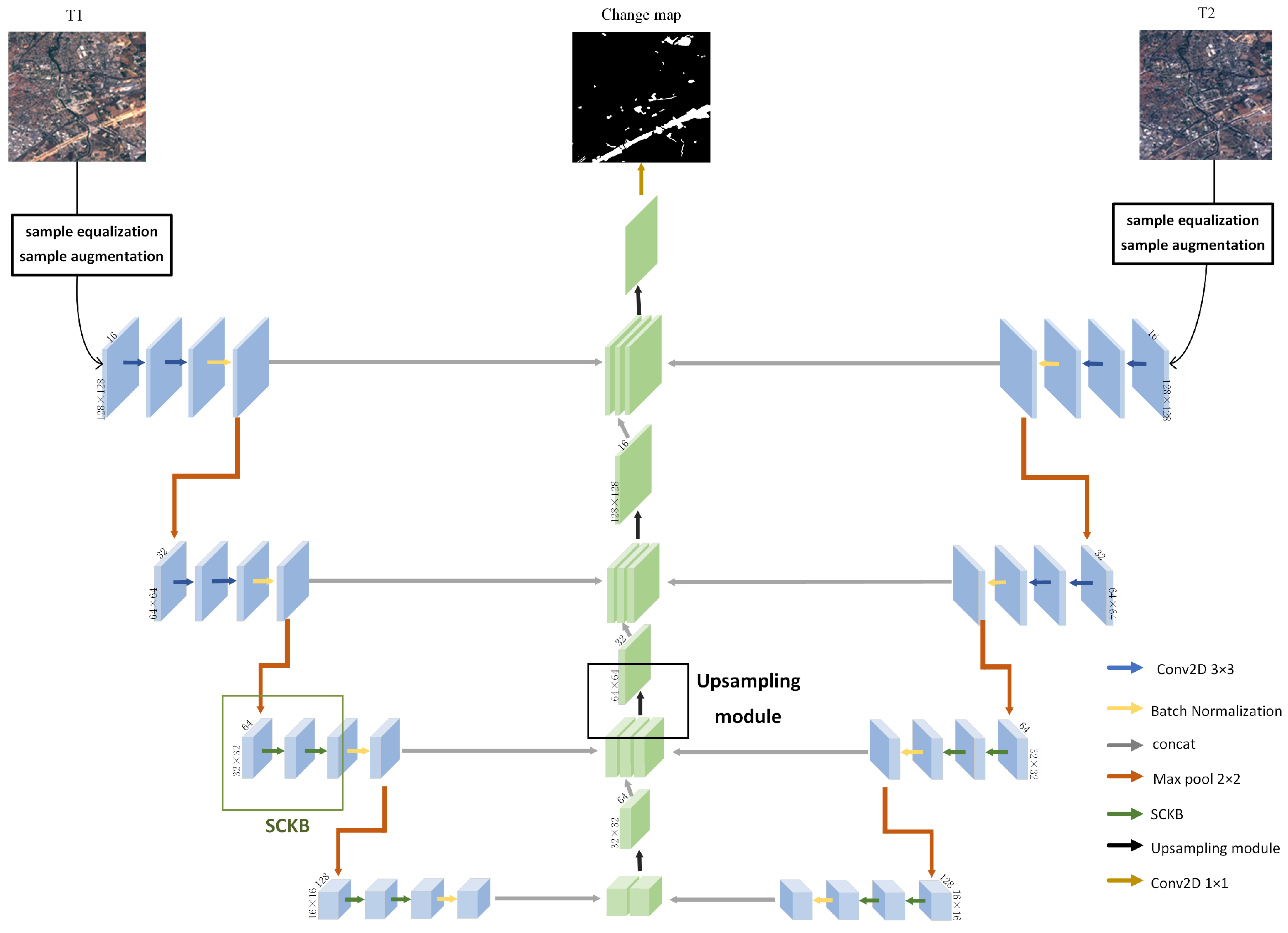
To effectively extract adaptive multi-scale features, resolve small range misclassification, and refine classification boundaries, a multispectral image change detection algorithm is proposed, whose framework is shown in Figure 1. The first step is to use sample equalization and sample augmentation to reduce the impact of sample imbalance on MSAK-Net. The second step trains MSAK-Net in an end-to-end manner and outputs a change probability map. The third step is to construct the unary potential function and the pair-wise potential function of fully connected conditional random fields (FC-CRF) with change probability map and multimodal difference map. The multimodal conditional random field is used to fully consider the correlation information between pixels, and change detection result is obtained.

The loss function of MSAK-Net using weighted cross-entropy loss is:

$$Loss=\frac{1}{N}\sum _{i=1}^N-t_{i}log\left(y_i\right)w_c-\left(1-t_i\right)log\left(1-y_i\right)$$

(1)

where $t_i$ represents the label of the ith pixel. When the ith pixel belongs to the changing pixel, $t_i$ is 1, otherwise $t_i$ is 0. $y_i$ represents the prediction result of MSAK-Net for the ith pixel, because the activation function of the last layer of the network is Sigmoid, so the value of $y_i$ is a probability between zero and one. The larger the $y_i$, the greater the probability that MSAK-Net considers the pixel to belong to the changing area. On the contrary, $1-y_i$ represents the probability that MSAK-Net predicts a non-changing pixel. It can be seen from the above formula that the optimization process of cross entropy is to increase the predicted probability $y_i$ of the change pixel corresponding to $t_i=1$, and increase the predicted probability $1-y_i$ of the non-change pixel corresponding to $t_i=0$. 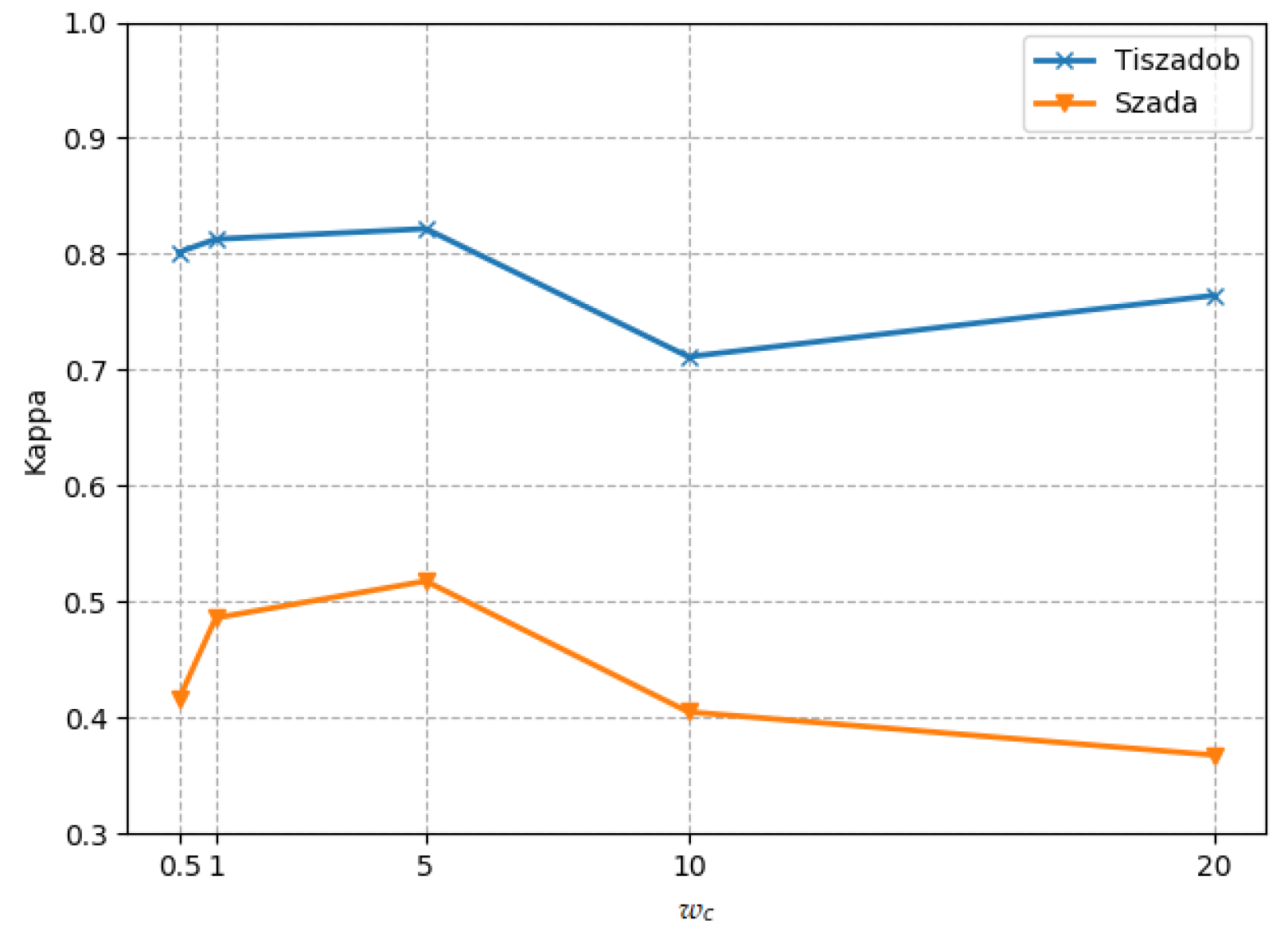$w_c$ is the class weight, which is generally the ratio of the number of non-changing samples to the number of changing samples, usually a value greater than 1. We first set it empirically to 5. In Section 5.3, we detail the effect of this weight parameter on the experimental results The weighted cross-entropy is to give a class weight when calculating the cross-entropy of the change class samples with a small number of samples. In this way, the cross entropy calculated by the change samples is larger, which makes the network pay more attention to the change samples, and can improve the recall rate of detection.

2.2. The Architecture of the MSAK-Net

Since change detection can be treated as a binary image segmentation, MSAK-Net adopts U-net as the backbone, which is an advanced image segmentation network. U-Net is divided into encoding path and decoding path, but the single encoding path limits the full use of original information from dual-temporal multispectral images. Some scholars extract the difference information, merge the dual-temporal multispectral images into a single difference features map, and then perform deep feature extraction through the encoding path. Another method is to superimpose the dual-temporal multispectral images along the channel dimension, and then input the encoding path. In order to preserve the original features of the dual-temporal multispectral images, we extend the encoding path of the U-Net. A weight-sharing bilateral encoding path is designed to extract independent features of two images without introducing additional parameters. The encoding path consists of four layers of convolutional modules, and the architecture of MSAK-Net is shown in Figure 2. The first two convolutional modules map the original image space into a high-dimensional feature space and consist of two convolutional layers with $3\times 3$ convolution kernels and a batch normalization layer. The next two layers of convolutional networks use two consecutive SCKBs to extract rich multiscale features, and then a batch normalization layer is used to prevent overfitting. A max pooling layer is set between every two layers convolutional module to filter out robust high-dimensional features. Each convolutional modules reduces the resolution of the output feature map to half of the input feature map, but doubles the number of channels.

The decoding path consists of four upsampling modules (UM) introduced in Section 2.4. Our proposed change detection framework preserves skip connections in U-Net networks. The shallow features and deep features are superimposed along the channel dimension and handed over to the subsequent channel attention for channel reorganization. The input of the first upsampling module is the superposition of the results of the two encoding paths. The input features of the latter three upsampling modules are directly superimposed by the output of the previous upsampling module and the output features of the two encoding paths of the same level. In contrast to the change of feature maps in the encoding path, each upsampling module in the decoding path doubles the feature map resolution. The output features of the last upsampling module go through a convolutional layer with a $1\times 1$ convolution kernel to adjust the number of channels of the final change detection map.

In the MSAK-Net, all convolutional layers use the ReLU activation function to alleviate the gradient disappearance, except that the last convolutional layer in the decoding path uses the Sigmoid activation function to calculate the probability intensity of the change map.

2.3. Selective Convolution Kernel Block

In response to the above situation, some scholars proposed using the Inception network to extract spatial features of different sizes [41]. The main idea of the Inception network is to improve the network performance by increasing the width of the network. The network uses $1\times 1$, $3\times 3$, and $5\times 5$ convolution kernels to extract features of different scales, and finally fuses multi-scale features through concat operation. Because the weights of each branch in the Inception network are the same, the network pays the same attention to features of different sizes. However, an appropriate weight allocation strategy should depend on the application scenario. Focusing on the above issues, we adopted a selective convolution kernel block (SCKB) to extract multi-scale features with adaptive weights from multispectral images. The structure of SCKB is shown in Figure 3.

The SCKB is divided into three convolution branches, each of which includes a convolution layer, a batch normalization layer, and an activation layer. The size of the convolution kernel in each convolutional layer is $3\times 3$, $5\times 5$ and $7\times 7$, respectively, corresponding to different receptive fields, which are used to extract features of three sizes. Suppose the input feature map is F, and the three sizes of feature maps are $U_1$, $U_2$, and $U_3$. Before calculating the weight of the convolution kernel, it is necessary to integrate the feature information of the three branches. The calculation formula of the multi-scale feature map U is:

$$U=\left[U_1;U_2;U_3\right]=\left[{Conv}^{3\times 3}\left(F\right);{Conv}^{5\times 5}\left(F\right);{Conv}^{7\times 7}\left(F\right)\right]$$

(2)

Assuming that the size of the input feature map F is $(w,h,c)$, the size of the deep features obtained by the three convolution branches remains unchanged. These three deep features are superimposed on the channel dimension through the concat operation to obtain a multi-scale feature U with a size of $(w,h,3c)$. The global information is encoded by global average pooling, and then a one-dimensional feature vector S is generated. The cth element of the feature vector S is calculated as follows:

$$S_c=AvgPool\left(U\right)=\frac{1}{h\times w}\sum _{i=1}^h\sum _{j=1}^w{U}_c(i,j)$$

(3)

Then two $1D$ convolutions are introduced to fuse all the statistical information to merge the interdependence between the channels in the feature vector S, thereby enhancing the information expression of the feature map of a certain scale. There is dimension scaling in the above process, and the output of the second $1D$ convolution is reshaped into a score matrix of size $(3,c)$. The score matrix is mapped into a weight coefficient matrix through Softmax calculation, and the sum of the three values in each column is one, which corresponds to the weight of the output results of the three convolution kernels at the channel. The weight coefficient matrix is obtained by the network through learning, and automatically assigns the most appropriate weights to the multi-scale features of three different convolution kernels. Finally, the weighted value of each feature map and the corresponding weight is calculated to obtain multi-scale fusion features.

The SCKB automatically adjusts the weights assigned to the three multi-scale features $U_1$, $U_2$, and $U_3$ according to different application scenarios, thus enabling the network to choose the most appropriate convolution kernel size.

2.4. Attention Module-Based Upsampling Unit

Although CNN can extract rich high-dimensional features from multispectral images, not all high-dimensional features contain useful change information, and irrelevant high-dimensional features can also bring challenges to change detection. In addition, in order to improve the use of information and prevent the loss of detailed information, U-Net use skip connections to reorganize the shallow features in the encoding path and their corresponding deep features in the decoding path [42]. However, a large number of features unrelated to change detection are also present in the shallow features with local information. Therefore, Attention Module (AM) is introduced to enhance the use of useful information. The AM is inspired by the perceptual process of the human visual system. The essence of AM is to make the network learn an attention weight. The weight corresponding to the important feature is larger, and the subsequent network will give it more attention. We added the Channel Attention Mechanism (CAM) and the Spatial Attention Mechanism (SAM) to the upsampling module of the U-Net, and designed an attention module-based Upsampling Module (UM).

An illustration of the UM is shown in Figure 4. The channel attention mechanism can filter the relevant feature channels containing changing information in shallow features and deep features, and suppress the feature expression of channels containing redundant information. Since the input features of the UM are obtained by simple channel stacking of shallow features and deep features, it is first necessary to use CAM to optimize the channel dimension of the input features. The importance of each channel is encoded in a one-dimensional channel weight vector, and the weight coefficient of each channel is automatically learned by the network. The specific calculation process is as follows:

$$M_c=\sigma (MLP(AvgPool\left(F\right))+MLP(MaxPool\left(F\right)))$$

(4)

Here, F represents the input feature, and $M_c$ represents the weight vector of channel attention mechanism. First, perform max pooling and average pooling on the spatial dimension of F, and obtain two feature vectors with the same length as the number of channels in F. The feature vectors extracted by the two pooling operations are different. The max pooling is to obtain the most distinguishing features on each channel, and the average pooling is to calculate the global information of each channel. The two feature vectors are fed into a multilayer perceptron (MLP), respectively, and then the two output results are added at the pixel level. The addition result is mapped to a weight vector between zero and one by the Sigmoid activation function, and the value on each weight vector represents the importance of the corresponding feature channel. $F_o^c$ is used as the output feature after CAM optimization, the optimization method of the final reorganization feature of channel attention mechanism is as follows:

$$F_o^c=F\otimes M_c$$

(5)

Here, ⊗ is an element-wise multiply operation. Before the deep features are transferred to the next upsampling module, in order to enable the transposed convolutional layer to learn more significantly changing features from the feature map, a spatial attention mechanism is used to optimize and reorganize the feature map in pixel dimension.

Similar to CAM, SAM encodes the information at each pixel position in the input feature, and the network adaptively learns the spatial attention map. The structure of the spatial attention mechanism is shown in the SAM dotted box in Figure 4. The calculation method of the spatial attention map is as follows:

$$M_s=\sigma (Conv2D\left([AvgPool\left(F\right);MaxPool\left(F\right)]\right))$$

(6)

where F represents the input feature and $M_s$ represents the spatial attention map. Similar to CAM, the input features are first encoded, average pooling obtains global information, and max pooling extracts robust information. Both pooling operations are one-dimensional pooling in the channel dimension, and finally two feature maps of size $(w,h,1)$ are obtained. The $[;]$ in Formula (6) represents the concat operation. We superimpose feature maps encoded by two pooling layers into a $(w,h,2)$ feature map. Then, the information is fused through a $2D$ convolution with a convolution kernel size of $7\times 7$, and finally the Sigmoid activation function is used to obtain the spatial attention map. After obtaining the spatial attention map, the calculation method of the spatial reorganization feature is as follows:

$$F_o^s=F\otimes M_s$$

(7)

Channel attention mechanism enables the selective fusion of shallow features and deep features in U-Net results, while spatial attention mechanism suppresses the feature information of non-changing pixels and enhances the difference features of changing pixels. After the optimization of channel attention mechanism and spatial attention mechanism, the feature map has better expression of change information in both channel dimension and spatial dimension. The optimization process of the entire module requires the introduction of additional computation and parameters with just two MLPs and one $2D$ convolutional layer. However, it can greatly improve the significant expression of changing features, which improves the accuracy and generality of the model. Our proposed upsampling module restores the lost pixels of the image by transposed convolution after the feature map is optimized by attention mechanism.

2.5. Secondary Classification Method Based on Multimodal Conditional Random Field

MSAK-Net has been able to achieve the classification and localization of change pixels, but there is still the problem of inaccurate localization due to information loss. In response to this problem, we use multimodal conditional random field (MCRF) to perform secondary classification on the results of MSAK-Net. The fully connected conditional random field (FC-CRF) is the optimization of the conditional random field, which overcomes the limitation of no remote dependence in the conditional random field by establishing the connection relationship between all the pixels in the image. The main idea of FC-CRF is to regard all pixels in the image as random variables in the random field model and to use an energy function to define the relationship between the pixels to describe the spatial correlation in the image, and map a set of input random variables to another set of random variables through modeling. At present, many related literatures have proved that using FC-CRF as the post-processing of the depth neural network can better recover the local information, so as to optimize the salt-and-pepper noise points in the classified image, fix fine mis-segmented areas, and obtain a more detailed segmentation boundary [15,16,43,44].

In the change detection, it is assumed that the input images $I_1$ and $I_2$ have N pixels, respectively, and $I_d$ is the difference map of $I_1$ and $I_2$. Vector $X=\left(X_1,X_2,\dots ,X_N\right)$ is used to represent the classification result of the network output, and $X_i$ represents the category (change, non-change) of the ith pixel. The output result of FC-CRF is represented by $Y=\left(Y_1,Y_2,\dots ,Y_N\right)$, and $Y_i$ represents the result of the secondary classification of the ith pixel. The probability distribution function of a conditional random field conforms to the Gibbs distribution, and the Gibbs distribution is calculated by the product of a series of non-negative energy functions of maximal cliques in the undirected graph model, so the probability distribution of the FC-CRF output Y is defined as follows:

$$E(Y\mid X)=\sum _{i=1}^N{\varphi }_u\left(x_i\right)+\sum _{i<j}{\varphi }_p\left(x_i,x_j\right)$$

(8)

where i and j range from 1 to N, ${\varphi }_u$ represent unary potential function, and ${\varphi }_p$ represent pair-wise potential function. ${\varphi }_u$ is usually calculated from the output of MSAK-Net, and the formula is:

$${\varphi }_u\left(x_i\right)=-logP\left(x_i\right)$$

(9)

$P\left(x_i\right)$ represents the probability intensity of MSAK-Net that the pixel i belongs to the change pixel. The result of MSAK-Net contains more noise points and discontinuities, so it is necessary to introduce pair-wise potential function to consider the positional relationship between pixels. Most of the current pair-wise potential function are defined by the difference image $I_d$, and only considering a single difference information to construct pair-wise potential function is likely to cause information loss. Therefore, we use the multimodal information as the input information of FC-CRF and propose a new pair-wise potential function to calculate the secondary classification results. The redefined pair-wise potential function is expressed as:

$${\varphi }_p\left(x_i,x_j\right)=\sum _{i<j}{\alpha }_i{\varphi }_{cvs.a}\left(x_i,x_j\right)+\sum _{i<j}{\beta }_i{\varphi }_{sa}\left(x_i,x_j\right)$$

(10)

where ${\varphi }_{cvs.a}\left(x_i,x_j\right)$ and ${\varphi }_{sa}\left(x_i,x_j\right)$ are the pair-wise potential functions defined according to the grayscale difference map extracted by change vector analysis (CVA) and the spectral difference map calculated by spectral angle (SA). ${\alpha }_i$ and ${\beta }_i$ are the weights of the two potential functions, respectively. They are usually set to 1, so as to balance the information provided by both, i.e., the proportion of the two difference information is the same weight. Taking ${\varphi }_{cvs.a}\left(x_i,x_j\right)$ as an example, the detailed calculation formula is:

$${\varphi }_{cvs.a}\left(x_i,x_j\right)=\mu \left(x_i,x_j\right)\sum _{m=1}^K{w}^{\left(m\right)}{k}^{\left(m\right)}\left(f_i,f_j\right)$$

(11)

Here, $\mu \left(x_i,x_j\right)$ is a label, $\mu \left(x_i,x_j\right)=1$ if $x_i\ne x_j$ and zero otherwise. K represents the number of gaussian kernels. $w^{\left(m\right)}$ is the weight coefficient of $k^{\left(m\right)}\left(f_i,f_j\right)$. $f_i$ and $f_j$ are the feature vectors corresponding to pixel i and j. The gaussian kernels are defined as follows:

$$k\left(f_i,f_j\right)=w_{1}exp\left(-\frac{{∥c_i-c_j∥}_2^2}{2{\sigma }_{\alpha }^2}-\frac{{∥d_i-d_j∥}_2^2}{2{\sigma }_{\beta }^2}\right)+w_{2}exp\left(-\frac{{∥c_i-c_j∥}_2^2}{2{\sigma }_{\gamma }^2}\right)$$

(12)

where $c_i$ represents the position vector of pixel i, and $d_i$ represents the difference intensity of pixel i in the CVA. The first gaussian kernel is used to define whether adjacent pixels with similar gray values in the difference map are of the same class. ${\sigma }_{\alpha }$ and ${\sigma }_{\beta }$ are gaussian kernel parameters. The second Gaussian kernel is used to smooth the boundary and noise of the classification result, and the smoothing effect is determined by the parameter ${\sigma }_{\gamma }$. $w_1$ and $w_2$ are the weights of the above two Gaussian kernels. Calculation process of ${\varphi }_{sa}\left(x_i,x_j\right)$ is the same as that of ${\varphi }_{cvs.a}\left(x_i,x_j\right)$, the difference is that ${\varphi }_{sa}\left(x_i,x_j\right)$ uses SA spectral difference map to define the difference intensity. Finally, the class label of each pixel is derived using mean field approximation algorithm [45].

3. Experiment Settings

This section will introduce the datasets used in the experiment, the experimental settings, the selected comparison methods and the evaluation index of the experimental results.

3.1. Datasets Description

Two datasets are selected for experiments, and the details are introduced as follows.

OSCD dataset: The first dataset comes from the Onera Satellite Change Detection (OSCD) dataset of the French Aeronautics and Space Administration [46]. The public dataset contains 24 pairs of multispectral images taken from the Sentinel-2 satellite between 2015 and 2018 at locations around the world, including the United States, Europe, and Asia. Each original multispectral image contains 13 bands, but four of them have a spatial resolution of 10 m, six have a spatial resolution of 20 m, and the remaining three have a spatial resolution of 60 m. The lower-resolution bands are upsampled to maintain the same image size as the other bands. Since the spatial resolution of the last three bands is too low, only 10 bands with high spatial resolution in the OSCD dataset are selected in our experiments. Two pairs of multispectral images captured in the OSCD dataset in Montpellier and Lasvegas were selected for testing and validation. The size of Montpellier is $451\times 426$, one third of the image is taken as the validation set, and the remaining two thirds are used as the test set. The size of the Lasvegas image is $816\times 704$, and the validation set is also a third of it. The ground truth maps of Montpellier and Lasvegas are shown in Figure 5 and Figure 6. The dataset focuses on changes in urban areas. In the ground truth map, complex urban change categories such as new buildings and road changes are manually marked, while natural changes (such as vegetation growth and seaweed changes) are ignored.

There are a total of 24 pairs of multispectral images in the OSCD dataset, and we crop the 22 pairs of images other than the test set and the validation set into $128\times 128$ image patches for network training. We represent the proportion of change pixels in the 1590 training samples in the form of a histogram. As shown in Figure 7a, the OSCD dataset has a serious imbalance of positive and negative samples. The proportion of change pixels in most training samples is less than 5%, and the number of non-change pixels in the entire training set is approximately 33 times the number of pixels that change. If data enhancement is performed directly on all training samples, the non-change area will also be enhanced, and the entire ratio of positive and negative samples remains unchanged. The direct use of this dataset by MSAK-Net can easily lead to overfitting and reduce the general fitting ability of the model.

Therefore, we need to selectively enhance the samples when performing data augmentation. Specifically, if the proportion of change pixels in the training sample is below 1%, it is filtered so that it does not participate in network training. If the proportion of change pixels in the training sample is more than 5%, image enhancement is used on it, and each training sample is rotated and flipped by 90°, 180°, and 270°. After sample equalization and data enhancement, 3129 training samples are finally obtained, and the number of non-changing pixels in the training set is 9.7 times that of changing pixels. This makes the distribution of positive and negative sample data in the training sample more balanced. The histogram of the proportion of change pixels in the training samples is shown in Figure 7b.

SZTAKI airchange benchmark: The second dataset, SZTAKI AirChange Benchmark (ACD), comes from the public dataset of the DEVA laboratory and contains 13 pairs of bi-temporal multispectral images. Each image has three bands of RGB, the image size is $952\times 640$, and the spatial resolution is 1.5 m. All images provide ground truth maps for reference. The changed areas of this dataset mainly include newly built houses, construction areas, newly planted trees, new farmland, etc. In the ground truth map, white pixels are used to represent the above-mentioned changed areas, and black pixels are non-changed areas. At present, this public dataset has been widely used in the methods of other scholars. We also adopt the same training set division method as others, using 11 pairs of multispectral images as the network training set, and images from the two regions of Tiszadob and Szada for testing and validation. The ground truth maps of the ACD dataset used for testing and validation are shown in Figure 8 and Figure 9.

We also crop 11 pairs of training images in the ACD dataset into 1170 training samples of $128\times 128$ size, and first analyze the distribution of changed pixels in the original training samples. As shown in Figure 10a, this dataset also has the problem of sample imbalance. The training samples that only contain non-changing regions are filtered, and the remaining samples are augmented by data to obtain a total of 4266 training samples. The balanced histogram is shown in Figure 10b, and the number of non-changing samples is 12 times that of changing samples.

3.2. Experimental Setup

All experiments used the Tensorflow open-source framework under the Ubuntu operating system. The learning rate of the network model can have an important impact on the training process. In the initial stage of network training, a large learning rate should be set to make the network parameters converge faster, and in the later stage of training, a small learning rate should be given to avoid the situation that the network cannot be converged due to oscillation. Therefore, we set the initial value of the learning rate to 1e ${}^{-4}$. The network is trained using Adam as the optimizer, and the Adam optimization algorithm reduces the learning rate according to the current number of iterations. The batch size of the network is set to 8. The smaller batch size makes the optimization direction of the network more accurate for each training, and the number of training iterations is 150.

3.3. Compared Methods

In this research, the proposed MSAK-Net-MCRF and several state-of-the-art multispectral change detection methods are compared experimentally on two datasets. The principle of choosing these comparison algorithms is that they adopt different network frameworks or different feature fusion methods, and have good performance and detection effect. These comparison algorithms are listed as follows:

•

Fully Convolutional Siamese-Concatenation (FC-Siam-conc)

This method belongs to a typical late fusion method proposed by Rodrigo et al. [27]. First, the siamese network is used to extract the high-dimensional features in the bi-temporal image, and then the bi-temporal high-dimensional features are superimposed in the channel dimension, and then input to the discriminator to detect the change features.

•

Fully Convolutional Siamese-Difference (FC-Siam-diff)

This method is similar to the network structure of FC-Siam-conc, except that the input to the discriminator is the absolute value of the difference between two high-dimensional features.

•

U-Net

This method adopts the U-Net network structure for change detection, but considering the size of the input training samples, the network only contains four max pooling layers and four upsampling layers. Furthermore, the input data of the encoding path is spliced by early fusion.

•

Deep Siamese Multiscale Convolutional Network (DSMS-CN)

The algorithm is proposed by Chen Wu et al. [32]. This is the first time that Inception module is exploited for Siamese neural network and four convolutional branches are used to extract deep features at different scales.

•

Densely connected siamese network (SNUNet)

SNUNet, proposed by Fang et al. [38], is a combination of Siamese network and NestedUNet with its proposed ensemble channel attention module (ECAM) added to it for deep monitoring.

3.4. Evaluation Metrics

In order to quantitatively evaluate the performance of different change detection algorithm, Precision (P), Recall (R), Accuracy ($ACC$), F1 coefficient ($F_1$), and Kappa coefficient ($KC$) are used as evaluation indicators to measure the performance of different algorithms. P refers to the correct proportion of the changed pixels predicted by the algorithm. R refers to the proportion of pixels that can be correctly predicted by the algorithm among all changed pixels. The choice of both P and R depends on different application scenarios. When the importance of the changed pixels is high, it is better to generate more false alarm rates and to detect all the real changed pixels as much as possible, we can consider choosing an algorithm with a higher R. When the changed pixels predicted by the algorithm need to have a higher accuracy, an algorithm with a higher P can be used. P and R are calculated as follows:

$$P=\frac{TP}{TP+FP}$$

(13)

$$R=\frac{TP}{TP+FN}$$

(14)

where $TP$, $FP$, $TN$, and $FN$ denote the number of true positives, the number of false positives, the number of true negatives, and the number of false negatives, respectively.

$ACC$ refers to the proportion of correctly classified samples to the total number of samples. Accuracy is the simplest and most intuitive evaluation index in classification problems, but when the proportion of samples in different categories is very uneven, the category with a large proportion often becomes the most important factor affecting the accuracy. $ACC$ are calculated as follows:

$$ACC=\frac{TP+TN}{TP+FP+TN+FN}$$

(15)

Ideally, it is desirable to obtain both high P and R, but it is difficult to achieve in general. We need to make a trade-off between the two indicators. In order to balance P and R, the weighted average of the two is used to measure, which is $F_1$, and the calculation formula is as follows:

$$F_1=\left(1+{\beta }^2\right)\times \frac{P\times R}{{\beta }^2\times P+R}$$

(16)

where $\beta$ represents the weight, which is generally set to 1. The higher the $\beta$, the greater the weight of R; conversely, the greater the weight of P.

In research, the $KC$ can also be used to measure the performance of the algorithm uniformly, and its calculation formula is:

$$KC=\frac{OA-P_e}{1-P_e}$$

(17)

$$OA=\frac{TP+TN}{TP+TN+FP+FN}$$

(18)

$$P_e=\frac{N_c\times (TP+FP)+N_u\times (TN+FN)}{{(TP+FP+TN+FN)}^2}$$

(19)

where, $N_c$ indicates the total number of real changed pixels, $N_u$ is the total number of real unchanged pixels. The larger the value of $KC$, the higher the accuracy of the algorithm.

4. Results

In this section, the effectiveness of MSAK-Net-MCRF is verified by comparative experiments. These experiments were performed on OSCD and SZTAKI datasets.

4.1. Experimental Result and Analysis on the OSCD Dataset

Two sets of bi-temporal multispectral images with complex ground objects are chosen from the OSCD dataset, and the experimental results are shown in Figure 11 and Figure 12. Meanwhile, for quantitative comparisons, five quantitative metrics are summarized in

Table 1. Experimental results of state-of-the-art methods on OSCD dataset.

Test Set	Metric	FC-Siam-Conc	FC-Siam-Diff	U-Net	DSMS-CN	SNUNet	MSAK-Net-MCRF
Montpellier	Precision	0.7476	0.7375	0.8438	0.5070	0.7895	0.7482
	Recall	0.6503	0.6895	0.5422	0.7694	0.5991	0.7751
	Acc	0.9506	0.9518	0.9516	0.9131	0.9514	0.9593
	F1	0.6956	0.7127	0.6602	0.6112	0.6813	0.7614
	Kappa	0.6689	0.6865	0.6355	0.5658	0.6555	0.7392
Lasvegas	Precision	0.6619	0.6822	0.7198	0.6388	0.7586	0.7689
	Recall	0.4584	0.6582	0.2610	0.7983	0.5369	0.6624
	Acc	0.9356	0.9464	0.9305	0.9460	0.9476	0.9556
	F1	0.5417	0.6700	0.3831	0.7097	0.6288	0.7117
	Kappa	0.5084	0.6409	0.3546	0.6804	0.6015	0.6879

. Figure 11 shows the experimental results of six change detection algorithms on the OSCD-Montpellier. It can be observed that the four methods of FC-Siam-conc, FC-Siam-diff, U-Net and SNUNet have obvious discontinuities in the detection of roads. This is because they only use a single-scale convolution kernel for change detection, which cannot effectively extract changing features, resulting in incomplete outlines of changing objects. Although DSMS-CN can completely detect road changes and find most of the real changing pixels, this method does not use attention machine to screen out irrelevant information in high-dimensional fusion features after using Siamese network to extract multi-scale features. The deep features of the network contain noise information in the original image, so the network’s identification of pseudo-change features is inaccurate, resulting in two false detection areas in the red box. MSAK-Net-MCRF not only completely extracts the road change area, but also maintains a better detection contour and the lowest false detection rate, so that the precision and recall are in a balanced state. The two comprehensive indexes of F1 coefficient and Kappa coefficient are 0.7614 and 0.7392, respectively, and the best change detection effect is achieved.

Figure 12 shows the experimental results of six change detection algorithms on the OSCD-Lasvegas. There are many isolated change pixels in the ground truth map, and the overall change area is relatively discrete. How to accurately identify small changes is the challenge to change detection on the dataset. It can be observed that using the U-Net for change detection has the worst effect, and there are a large number of missed pixels. Due to the use of attention mechanism, SNUNet and MSAK-Net-MCRF enhance the spatial information and channel information of regions of interest, while weaken irrelevant regions and channels, thus achieving better precision. Both DSMS-CN and MSAK-Net-MCRF extract multi-scale features for change detection. The two methods are also better than other methods in visual effect and detection accuracy. It is worth noting that DSMS-CN has the highest recall, and most of the changed pixels in the OSCD-Lasvegas can be detected by this method, but this method produces more false detection points. MSAK-Net-MCRF has the least false detection points and also has a satisfactory recall, so it is also better than the DSMS-CN method in the two comprehensive indicators of F1 and Kappa.

4.2. Experimental Result and Analysis on SZTAKI Dataset

The qualitative results of six change detection algorithms on the SZTAKI dataset are shown in Figure 13 and Figure 14. Observing the ground truth map in Figure 13a, notice that the change region of the Tiszadob is a large-scale change with regular and continuous boundaries. FC-Siam-conc and MSAK-Net-MCRF have the best contour integrity and the best internal homogeneity. The outstanding performance of FC-Siam-conc and MSAK-Net-MCRF makes them have the highest precision and recall, respectively. However, FC-Siam-conc produces obvious salt-and-pepper noise in other regions, which makes this method inferior to MSAK-Net-MCRF in comprehensive performance. SNUNet also obtains good contour integrity, but due to its use of a single-scale convolution kernel, it generates a lot of salt-and-pepper noise and contour discontinuities in the lower and lower left corners of the resulting map. The other three methods identify a lot of changing pixels as non-changing pixels, and the internal consistency of change objects on the change map is poor. According to

Table 2. Experimental results of state-of-the-art methods on SZTAKI dataset.

Test set	Metric	FC-Siam-Conc	FC-Siam-Diff	U-Net	DSMS-CN	SNUNet	MSAK-Net-MCRF
Tiszadob	Precision	0.9428	0.7416	0.8933	0.7712	0.8607	0.7491
	Recall	0.7392	0.6869	0.6848	0.7955	0.7087	0.9920
	Acc	0.9476	0.9319	0.9319	0.9235	0.9438	0.9409
	F1	0.8287	0.7758	0.7753	0.7832	0.7773	0.8536
	Kappa	0.7983	0.7365	0.7360	0.7367	0.7455	0.8175
Szada	Precision	0.4316	0.4760	0.3709	0.4636	0.3688	0.5715
	Recall	0.4029	0.4602	0.3779	0.6048	0.4759	0.5139
	Acc	0.9409	0.9452	0.9477	0.9426	0.9624	0.9554
	F1	0.4168	0.4680	0.3744	0.5249	0.4156	0.5412
	Kappa	0.3858	0.4391	0.3584	0.4949	0.3965	0.5172

, the recall of MSAK-Net-MCRF is as high as 0.992, which is much higher than the other four methods. This means that almost all real changing pixels can be completely detected. However, the wrong production detected two false change areas in the lower left corner and upper right corner, resulting in a decrease in the F1 coefficient and Kappa coefficient, but still increased by 2.49%and 1.92%. We think this is due to the fact that the convolution kernels of SCKB are fixed in size, such as $3\times 3$, $5\times 5$ and $7\times 7$. Although our proposed SCKB module can assign adaptive weights to different scales, we only use convolution kernels of $3\times 3$, $5\times 5$ and $7\times 7$. Therefore, the detection effect may not be so good for some smaller targets, so there will be error detection areas as shown in the figure.

Szada of SZTAKI contains both small changing targets and large changing areas, and it is difficult to achieve good detection results on this test set. As can be seen from the result map, because SNUNet uses the attention mechanism to reorganize and enhance the spatial information and channel information, most of the change regions are detected. However, due to the loss of information in the deep layer of the neural network, it produces more noise at the edge and interior of the contour, which leads to its unsatisfactory detection results. DSMS-CN and MSAK-Net-MCRF use multi-branch convolutional paths to extract features of different scales, giving these two methods the highest accuracy and recall, respectively. We conclude that the detection performance of multi-scale convolutional networks is better than the other four methods using a single convolution kernel for both small objects and changing objects in large regions. Meanwhile, MSAK-Net-MCRF can flexibly adjust the influence of different convolutional branches on the network according to the input region. In addition, MSAK-NET-MCRF uses MCRF to make up for the lack of deep neural network information and reduce omissions. Therefore, MSAK-Net-MCRF has better self-adaptation than DSMS-CN, with F1 coefficient is increased by 1.6%, and the kappa is increased by 2.2%. This also verifies that the feature extraction capability of the Selective Convolution Kernel Block (SCKB) is stronger. However, for the left part of the result graph, we can see that MSAK-Net-MCRF does not well detect the roads in this area. In our analysis, this is due to the fact that the SCKB module is better at detecting objects with regular shapes and smooth boundaries, while the detection of irregular shapes such as roads is slightly worse.

5. Discussion

5.1. Ablation Study

Our proposed SCKB is used to extract multi-scale features, which adaptively allocates different weights to different size convolution kernels to achieve better detection results. The attention mechanism is introduced into the upsampling module to enhance useful spatial and channel information. MCRF is used to refine the boundary information of change objects, so as to obtain more accurate change detection results. We designed an ablation experiment to evaluate the performance of these three modules.

First of all, we verify the influence of post-processing MCRF on network results. Figure 15 and Figure 16 show ablation study of MCRF on two datasets.

Table 3. Ablation study of multimodal conditional random field on OSCD and SZTAKI datasets.

Test Set	Method	F1	Kappa
Montpellier of OSCD dataset	MSAK-Net	0.7599	0.7370
	MSAK-Net-MCRF	0.7614	0.7392
Lasvegas of OSCD dataset	MSAK-Net	0.7100	0.6856
	MSAK-Net-MCRF	0.7117	0.6879
Tiszadob of SZTAKI dataset	MSAK-Net	0.8514	0.8147
	MSAK-Net-MCRF	0.8536	0.8175
Szada of SZTAKI dataset	MSAK-Net	0.5407	0.5166
	MSAK-Net-MCRF	0.5412	0.5172

shows the impact of MCRF on the two comprehensive indicators. We can observe that MSAK-Net has achieved relatively satisfactory results. Combined with MCRF, the comprehensive performance of MSAK-Net can be further improved. This is because, when using MCRF, multimodal differential information is used to compensate for the local information lost by the deep network, which brings performance improvements.

In addition, we also studied the influence of ${\alpha }_i$ and ${\beta }_i$ values (in Formula (10)) of grayscale difference information (obtained by CVA) and spectral difference information (obtained by SA) on the experimental results in MCRF. We used the Tiszadob dataset to carry out the experiment. The experimental results are shown in

Table 4. Ablation study of ${\alpha }_i$ and ${\beta }_i$ on Tiszadob of OSCD datasets.

Kappa		${\mathit{\beta }}_{\mathit{i}}$
		0	0.5	1	2	3
${\mathbf{\alpha }}_{\mathbf{i}}$	0	0.8147	0.8155	0.8164	0.8175	0.8183
	0.5	0.8155	0.8164	0.8172	0.8179	0.8189
	1	0.8164	0.8172	0.8175	0.8184	0.8188
	2	0.8175	0.8179	0.8183	0.8188	0.8177
	3	0.8183	0.8189	0.8188	0.8177	0.8161

. As can be seen from the results, when both difference maps are not considered (i.e., both are 0), MCRF is not able to add more difference information to the network output results since it only uses the output of MSAK-Net to construct the unary potential function at this time, and thus has no improvement for the network results. When one weight is 0 (i.e., this difference map is not considered), the improvement of MCRF for accuracy increases as the other weight increases, due to the increasing amount of difference information it can provide. However, we also find that MCRF achieves the maximum improvement when both difference maps are considered (i.e., both are greater than 0). This is because MCRF using multimodal difference maps to construct pair-wise potential functions can extract the local variation features in the original image from unused aspects, while the input to the FC-CRF model has the effect of information complementarity.

In the experiment of the previous chapter, we set ${\alpha }_i={\beta }_i=1$. However, we can find that the experimental result is the best when ${\alpha }_i=3,{\beta }_i=0.5$ or ${\alpha }_i=0.5,{\beta }_i=3$, and the kappa reaches 0.8189, which is higher than the accuracy of our initial setting (0.8175). Furthermore, from the ablation experiment of MCRF, we can see that the Kappa value after removing the MCRF module is 0.8147, which is lower than the result when we set the weight arbitrarily. Therefore, we think that these two weight coefficients are robust to the experimental results, and the effect of MCRF is the best when ${\alpha }_i=3,{\beta }_i=0.5$ or ${\alpha }_{0.5}=3,{\beta }_i=3$.

After that, we verify the impact of SCKB and attention mechanism on the MSAK-Net network on the Tiszadob of SZTAKI dataset without the application of post-processing MCRF. Figure 17 shows ablation study of SCKB and attention mechanism on the MSAK-Net network.

Table 5. Ablation study of SCKB and attention mechanism of MSAK-Net on Tiazadob of SZTAKI datasets.

Method	F1	Kappa
MSAK-Net	0.8514	0.8147
MSAK-Net without SCKB	0.8306	0.7888
MSAK-Net without attention mechanism	0.8489	0.8129

shows the impact of SCKB and attention mechanism on the two comprehensive indicators. It can be seen from the table that MSAK-Net performs relatively poorly when removing SCKB or attention mechanism. As can be seen from the result diagram, for the SCKB module, due to the use of ordinary convolution instead of SCKB, the network loses the ability to extract multi-scale features, so its performance on Tiszadob data sets is poor, resulting in a large number of false detection and missed detection, but because it retains the attention mechanism, it performs well in internal consistency. For the attention mechanism, the network retains the SCKB, but removes the attention mechanism, so it performs well in detecting the integrity of the overall contour, but because the attention mechanism loses the enhancement and fusion of spatial information and channel information, there are internal inconsistencies, and there are many misdetection areas inside the contour.

5.2. Effect of Kernel Size in SCKB Module

In order to test the influence of SCKB module on the results more comprehensively, we also designed a set of experiments on convolution kernel size. In previous experiments, the convolution kernel size was empirically set to $3\times 3$, $5\times 5$ and $7\times 7$. To test the effect of convolution kernel size on the results in SCKB module, we set the convolution kernel size to three different sizes, respectively, and carried out experiments on Tiszadob datasets. The experimental results are shown in Figure 18. It can be seen from the experimental results that the accuracy of the network decreases with the increase of the convolution kernel size in the SCKB module. This is because in the deep layer of the network, the size of the feature map gradually shrinks after convolution and pooling, and a small piece of the feature map represents the large-scale target in the original image. At this time, the features of large-scale target can be extracted using small or moderate convolution kernel for convolution operation. However, when using too large receptive field (such as $9\times 9$), the extracted features contain not only large-scale target, but also surrounding irrelevant information, so that the extracted features contain too much irrelevant information and reduce the accuracy of the network.

5.3. Effect of Class Weight

For the loss function of MSAK-Net, the class weight $w_c$ indicates how much the model pays attention to change samples during training. In multispectral images, the proportion of changing areas is small, and there is a problem of sample imbalance, which easily makes the loss function fall into the local optimal value. Therefore, the class weight plays an important role in the training process of MSAK-Net. To verify the impact of $w_c$ on change detection, we explore the experimental results of different $w_c$ on the SZTAKI dataset, as illustrated in Figure 19. When $w_c$ is 0.5, MSAK-Net pays more attention to non-changing samples on training, and it is easy to increase Recall and Kappa. As $w_c$ increases, the detection rate for changing samples increases, hence the performance is improved. It is worth noting that Kappa reaches its maximum value when $w_c$ is 5, which means that the effect of changing samples reaches a state of equilibrium. However, the Kappa evaluation metrics show a downward trend with the further increase of parameter $w_c$. Hence, we set $w_c$ to 5.

5.4. Computation Time Analysis

To show the running cost and computational cost of the proposed algorithm, we employ a running time analysis to quantitatively analyze it. The calculation time is shown in

Table 6. Comparison of calculation time of six methods.

Method	Training Time (s/epoch)	Testing Time (s)
FC-Siam-conc	45.97	0.27
FC-Siam-diff	47.27	0.18
U-Net	55.98	0.40
DSMS-CN	42.08	5.84
SNUNet	62.60	1.73
MSAK-Net-MCRF	50.11	6.97

. The results show that MSAK-Net-MCRF has less training time compared to U-Net and SNUNet and more than the remaining comparison methods, but these time costs are acceptable due to the effectiveness of MSAK-Net-MCRF. The proposed method does not have an advantage in test time, because the MCRF post-processing needs to be used for secondary classification after the network test is completed, thereby reducing omissions.

6. Conclusions

In this paper, a multispectral change detection method based on multi-scale adaptive kernel network and multimodal conditional random field (MSAK-Net-MCRF) is proposed. Combined with the characteristics of multispectral images, a Selective Convolution Kernel Block (SCKB) that can adaptively assign weights is proposed to solve the problem of insufficient use of multi-scale information in current multispectral change detection methods using a single convolution kernel. First, the proposed MSAK-Net adopts U-Net with dual encoding paths as the overall framework, since the U-Net framework retains more original image information through skip connections. Furthermore, in order to overcome the problem of feature heterogeneity fusion, an attention mechanism is added to the decoding path to selectively fuse shallow features and deep features. Finally, the multimodal conditional random field is used to perform secondary classification on the detection results of the neural network, recover the local information lost by MSAK-Net, and make the final detection boundary more accurate. The effectiveness of MSAK-Net-MCRF is verified by analyzing the experimental results of five change detection methods on two public datasets. Compared with the other four state-of-the-art methods, the proposed approach achieves the best results on both comprehensive metrics.

References

1. Li, Y.; Peng, C.; Chen, Y.; Jiao, L.; Zhou, L.; Shang, R. A deep learning method for change detection in synthetic aperture radar images. IEEE Trans. Geosci. Remote Sens. 2019, 57, 5751–5763. [Google Scholar] [CrossRef]
2. Zhang, W.; Lu, X. The Spectral-Spatial Joint Learning for Change Detection in Multispectral Imagery. Remote Sens. 2019, 11, 240. [Google Scholar] [CrossRef] [Green Version]
3. Mou, L.; Bruzzone, L.; Zhu, X.X. Learning Spectral-Spatial-Temporal Features via a Recurrent Convolutional Neural Network for Change Detection in Multispectral Imagery. IEEE Trans. Geosci. Remote Sens. 2019, 57, 924–935. [Google Scholar] [CrossRef] [Green Version]
4. He, Y.; Jia, Z.; Yang, J.; Kasabov, N.K. Multispectral Image Change Detection Based on Single-Band Slow Feature Analysis. Remote Sens. 2021, 13, 2969. [Google Scholar] [CrossRef]
5. Shi, W.; Zhang, M.; Zhang, R.; Chen, S.; Zhan, Z. Change Detection Based on Artificial Intelligence: State-of-the-Art and Challenges. Remote Sens. 2020, 12, 1688. [Google Scholar] [CrossRef]
6. Panuju, D.R.; Paull, D.J.; Griffin, A.L. Change Detection Techniques Based on Multispectral Images for Investigating Land Cover Dynamics. Remote Sens. 2020, 12, 1781. [Google Scholar] [CrossRef]
7. Bovolo, F.; Bruzzone, L. A theoretical framework for unsupervised change detection based on change vector analysis in the polar domain. IEEE Trans. Geosci. Remote Sens. 2007, 45, 218–236. [Google Scholar] [CrossRef] [Green Version]
8. Nielsen, A.A.; Conradsen, K.; Simpson, J.J. Multivariate alteration detection (MAD) and MAF postprocessing in multispectral, bitemporal image data: New approaches to change detection studies. Remote Sens. Environ. 1998, 64, 1–19. [Google Scholar] [CrossRef] [Green Version]
9. Nielsen, A.A. The regularized iteratively reweighted MAD method for change detection in multi- and hyperspectral data. IEEE Trans. Image Process. 2007, 16, 463–478. [Google Scholar] [CrossRef] [PubMed] [Green Version]
10. Wu, C.; Du, B.; Zhang, L. Slow Feature Analysis for Change Detection in Multispectral Imagery. IEEE Trans. Geosci. Remote Sens. 2014, 52, 2858–2874. [Google Scholar] [CrossRef]
11. Bruzzone, L.; Prieto, D.F. An MRF approach to unsupervised change detection. In Proceedings of the 1999 International Conference on Image Processing (Cat. 99CH36348), Kobe, Japan, 24–28 October 1999; Volume 1, pp. 143–147. [Google Scholar]
12. Lv, P.; Zhong, Y.; Zhao, J.; Zhang, L. Unsupervised change detection based on hybrid conditional random field model for high spatial resolution remote sensing imagery. IEEE Trans. Geosci. Remote Sens. 2018, 56, 4002–4015. [Google Scholar] [CrossRef]
13. Hoberg, T.; Rottensteiner, F.; Feitosa, R.Q.; Heipke, C. Conditional random fields for multitemporal and multiscale classification of optical satellite imagery. IEEE Trans. Geosci. Remote Sens. 2014, 53, 659–673. [Google Scholar] [CrossRef]
14. Zhao, J.; Zhong, Y.; Shu, H.; Zhang, L. High-resolution image classification integrating spectral-spatial-location cues by conditional random fields. IEEE Trans. Image Process. 2016, 25, 4033–4045. [Google Scholar] [CrossRef] [PubMed]
15. Zhang, B.; Wang, C.; Shen, Y.; Liu, Y. Fully Connected Conditional Random Fields for High-Resolution Remote Sensing Land Use/Land Cover Classification with Convolutional Neural Networks. Remote Sens. 2018, 10, 1889. [Google Scholar] [CrossRef] [Green Version]
16. Krähenbühl, P.; Koltun, V. Efficient Inference in Fully Connected CRFs with Gaussian Edge Potentials. In Proceedings of the 24th International Conference on Neural Information Processing Systems, Granada, Spain, 12–15 December 2011; pp. 109–117. [Google Scholar]
17. Saha, S.; Solano-Correa, Y.T.; Bovolo, F.; Bruzzone, L. Unsupervised Deep Transfer Learning-Based Change Detection for HR Multispectral Images. IEEE Geosci. Remote Sens. Lett. 2021, 18, 856–860. [Google Scholar] [CrossRef]
18. Shafique, A.; Cao, G.; Khan, Z.; Asad, M.; Aslam, M. Deep learning-based change detection in remote sensing images: A review. Remote Sens. 2022, 14, 871. [Google Scholar] [CrossRef]
19. Liu, S.; Bruzzone, L.; Bovolo, F.; Du, P. Hierarchical unsupervised change detection in multitemporal hyperspectral images. IEEE Trans. Geosci. Remote Sens. 2014, 53, 244–260. [Google Scholar]
20. Ferraris, V.; Dobigeon, N.; Wei, Q.; Chabert, M. Detecting changes between optical images of different spatial and spectral resolutions: A fusion-based approach. IEEE Trans. Geosci. Remote Sens. 2017, 56, 1566–1578. [Google Scholar] [CrossRef]
21. Lin, Y.; Li, S.; Fang, L.; Ghamisi, P. Multispectral Change Detection With Bilinear Convolutional Neural Networks. IEEE Geosci. Remote Sens. Lett. 2020, 17, 1757–1761. [Google Scholar] [CrossRef]
22. Tan, K.; Zhang, Y.; Wang, X.; Chen, Y. Object-Based Change Detection Using Multiple Classifiers and Multi-Scale Uncertainty Analysis. Remote Sens. 2019, 11, 359. [Google Scholar] [CrossRef] [Green Version]
23. Zhang, C.; Yue, P.; Tapete, D.; Shangguan, B.; Wang, M.; Wu, Z. A multi-level context-guided classification method with object-based convolutional neural network for land cover classification using very high resolution remote sensing images. Int. J. Appl. Earth Obs. Geoinf. 2020, 88, 102086. [Google Scholar] [CrossRef]
24. Sun, S.; Mu, L.; Wang, L.; Liu, P. L-UNet: An LSTM Network for Remote Sensing Image Change Detection. IEEE Geosci. Remote Sens. Lett. 2022, 19, 1–5. [Google Scholar] [CrossRef]
25. Peng, D.; Bruzzone, L.; Zhang, Y.; Guan, H.; Ding, H.; Huang, X. SemiCDNet: A Semisupervised Convolutional Neural Network for Change Detection in High Resolution Remote-Sensing Images. IEEE Trans. Geosci. Remote Sens. 2021, 59, 5891–5906. [Google Scholar] [CrossRef]
26. Ji, S.; Wei, S.; Lu, M. Fully Convolutional Networks for Multisource Building Extraction From an Open Aerial and Satellite Imagery Data Set. IEEE Trans. Geosci. Remote Sens. 2019, 57, 574–586. [Google Scholar] [CrossRef]
27. Daudt, R.C.; Le Saux, B.; Boulch, A. Fully convolutional siamese networks for change detection. In Proceedings of the 2018 25th IEEE International Conference on Image Processing (ICIP), Athens, Greece, 7–10 October 2018; pp. 4063–4067. [Google Scholar]
28. Chen, H.; Wu, C.; Du, B.; Zhang, L.; Wang, L. Change Detection in Multisource VHR Images via Deep Siamese Convolutional Multiple-Layers Recurrent Neural Network. IEEE Trans. Geosci. Remote Sens. 2020, 58, 2848–2864. [Google Scholar] [CrossRef]
29. Kusetogullari, H.; Yavariabdi, A.; Celik, T. Unsupervised change detection in multitemporal multispectral satellite images using parallel particle swarm optimization. IEEE J. Sel. Top. Appl. Earth Obs. Remote Sens. 2015, 8, 2151–2164. [Google Scholar] [CrossRef]
30. Hou, B.; Wang, Y.; Liu, Q. Change Detection Based on Deep Features and Low Rank. IEEE Geosci. Remote Sens. Lett. 2017, 14, 2418–2422. [Google Scholar] [CrossRef]
31. Liu, T.; Yang, L.; Lunga, D. Change detection using deep learning approach with object-based image analysis. Remote Sens. Environ. 2021, 256, 112308. [Google Scholar] [CrossRef]
32. Chen, H.; Wu, C.; Du, B.; Zhang, L. Deep Siamese Multi-scale Convolutional Network for Change Detection in Multi-temporal VHR Images. In Proceedings of the 2019 10th International Workshop on the Analysis of Multitemporal Remote Sensing Images (Multitemp), Shanghai, China, 5–7 August 2019. [Google Scholar]
33. Song, A.; Choi, J. Fully convolutional networks with multiscale 3D filters and transfer learning for change detection in high spatial resolution satellite images. Remote Sens. 2020, 12, 799. [Google Scholar] [CrossRef] [Green Version]
34. Zhang, X.; He, L.; Qin, K.; Dang, Q.; Si, H.; Tang, X.; Jiao, L. SMD-Net: Siamese Multi-Scale Difference-Enhancement Network for Change Detection in Remote Sensing. Remote Sens. 2022, 14, 1580. [Google Scholar] [CrossRef]
35. Mnih, V.; Heess, N.; Graves, A. Recurrent models of visual attention. In Proceedings of the 27th International Conference on Neural Information Processing Systems-Volume 2, Montreal, Canada, 8–13 December 2014; pp. 2204–2212. [Google Scholar]
36. Zhang, C.; Yue, P.; Tapete, D.; Jiang, L.; Shangguan, B.; Huang, L.; Liu, G. A deeply supervised image fusion network for change detection in high resolution bi-temporal remote sensing images. ISPRS J. Photogramm. Remote Sens. 2020, 166, 183–200. [Google Scholar] [CrossRef]
37. Peng, X.; Zhong, R.; Li, Z.; Li, Q. Optical Remote Sensing Image Change Detection Based on Attention Mechanism and Image Difference. IEEE Trans. Geosci. Remote Sens. 2021, 59, 7296–7307. [Google Scholar] [CrossRef]
38. Fang, S.; Li, K.; Shao, J.; Li, Z. SNUNet-CD: A densely connected Siamese network for change detection of VHR images. IEEE Geosci. Remote Sens. Lett. 2021, 19, 1–5. [Google Scholar] [CrossRef]
39. Chen, H.; Shi, Z. A Spatial-Temporal Attention-Based Method and a New Dataset for Remote Sensing Image Change Detection. Remote Sens. 2020, 12, 1662. [Google Scholar] [CrossRef]
40. Woo, S.; Park, J.; Lee, J.Y.; Kweon, I.S. Cbam: Convolutional block attention module. In Proceedings of the European Conference on Computer Vision (ECCV), Munich, Germany, 8–14 September 2018; pp. 3–19. [Google Scholar]
41. Szegedy, C.; Liu, W.; Jia, Y.; Sermanet, P.; Reed, S.; Anguelov, D.; Erhan, D.; Vanhoucke, V.; Rabinovich, A. Going Deeper with Convolutions. In Proceedings of the 2015 IEEE Conference on Computer Vision and Pattern Recognition (CVPR), Boston, MA, USA, 7–12 June 2015; pp. 1–9. [Google Scholar] [CrossRef] [Green Version]
42. Zhang, Z.; Liu, Q.; Wang, Y. Road Extraction by Deep Residual U-Net. IEEE Geosci. Remote Sens. Lett. 2018, 15, 749–753. [Google Scholar] [CrossRef] [Green Version]
43. Shi, C.; Zhou, Y.; Qiu, B.; Guo, D.; Li, M. CloudU-Net: A Deep Convolutional Neural Network Architecture for Daytime and Nighttime Cloud Images’ Segmentation. IEEE Geosci. Remote Sens. Lett. 2021, 18, 1688–1692. [Google Scholar] [CrossRef]
44. Feng, W.; Sui, H.; Huang, W.; Xu, C.; An, K. Water Body Extraction From Very High-Resolution Remote Sensing Imagery Using Deep U-Net and a Superpixel-Based Conditional Random Field Model. IEEE Geosci. Remote Sens. Lett. 2019, 16, 618–622. [Google Scholar] [CrossRef]
45. Shi, W.; Zhang, M.; Ke, H.; Fang, X.; Zhan, Z.; Chen, S. Landslide Recognition by Deep Convolutional Neural Network and Change Detection. IEEE Trans. Geosci. Remote Sens. 2021, 59, 4654–4672. [Google Scholar] [CrossRef]
46. Jiang, H.; Peng, M.; Zhong, Y.; Xie, H.; Hao, Z.; Lin, J.; Ma, X.; Hu, X. A Survey on Deep Learning-Based Change Detection from High-Resolution Remote Sensing Images. Remote Sens. 2022, 14, 1552. [Google Scholar] [CrossRef]
Figure 1. The pipeline of the change detection algorithm.
Remotesensing 14 05368 g001
Figure 2. Architecture of the proposed MSAK-Net.
Remotesensing 14 05368 g002
Figure 3. Illustration of SCKB.
Remotesensing 14 05368 g003
Figure 4. Structure of Upsampling Module (UM).
Remotesensing 14 05368 g004
Figure 5. Montpellier of OSCD. (a) Pre-change. (b) Post-change. (c) ground truth map.
Remotesensing 14 05368 g005
Figure 6. Lasvegas of OSCD. (a) Pre-change. (b) Post-change. (c) ground truth map.
Remotesensing 14 05368 g006
Figure 7. Distribution of change pixels in OSCD. (a) Before sample equalization. (b) After sample equalization.
Remotesensing 14 05368 g007
Figure 8. Tiszadob of ACD. (a) Pre-change. (b) Post-change. (c) ground truth map.
Remotesensing 14 05368 g008
Figure 9. Szada of ACD. (a) Pre-change. (b) Post-change. (c) ground truth map.
Remotesensing 14 05368 g009
Figure 10. Distribution of change pixels in ACD. (a) Before sample equalization. (b) After sample equalization.
Remotesensing 14 05368 g010
Figure 11. Result examples of different change detection algorithms on the Montpellier of OSCD dataset. (a) ground truth map, (b) FC-Siam-conc, (c) FC-Siam-diff, (d) U-Net, (e) DSMS-CN, (f) SNUNet, (g) MSAK-Net-MCRF.
Remotesensing 14 05368 g011
Figure 12. Result examples of different change detection algorithms on the Lasvegas of OSCD dataset. (a) ground truth map, (b) FC-Siam-conc, (c) FC-Siam-diff, (d) U-Net, (e) DSMS-CN, (f) SNUNet, (g) MSAK-Net-MCRF.
Remotesensing 14 05368 g012
Figure 13. Result examples of different change detection algorithms on the Tiszadob of SZTAKI dataset. (a) ground truth map, (b) FC-Siam-conc, (c) FC-Siam-diff, (d) U-Net, (e) DSMS-CN, (f) SNUNet, (g) MSAK-Net-MCRF.
Remotesensing 14 05368 g013
Figure 14. Result examples of different change detection algorithms on the Szada of SZTAKI dataset. (a) ground truth map, (b) FC-Siam-conc, (c) FC-Siam-diff, (d) U-Net, (e) DSMS-CN, (f) SNUNet, (g) MSAK-Net-MCRF.
Remotesensing 14 05368 g014
Figure 15. Ablation study of multimodal conditional random field on the OSCD dataset. (a) MSAK-Net of Montpellier, (b) MSAK-Net-MCRF of Montpellier, (c) MSAK-Net of Lasvegas, (d) MSAK-Net-MCRF of Lasvegas.
Remotesensing 14 05368 g015
Figure 16. Ablation study of multimodal conditional random field on the SZTAKI dataset. (a) MSAK-Net of Tiszadob, (b) MSAK-Net-MCRF of Tiszadob, (c) MSAK-Net of Szada, (d) MSAK-Net-MCRF of Szada.
Remotesensing 14 05368 g016
Figure 17. Ablation study of SCKB and attention mechanism on Tiazadob of SZTAKI datasets. (a) ground truth map of Tiszadob, (b) MSAK-Net of Tiszadob, (c) MSAK-Net without SCKB, (d) MSAK-Net without attention mechanism.
Remotesensing 14 05368 g017
Figure 18. The effects of kernel size in SCKB module on the accuracy of MSAK-Net.
Remotesensing 14 05368 g018
Figure 19. The effects of parameter w c on the accuracy of MSAK-Net.
Remotesensing 14 05368 g019