Forest Biodiversity Monitoring Based on Remotely Sensed Spectral Diversity—A Review

Abstract

Forests are essential for global environmental well-being because of their rich provision of ecosystem services and regulating factors. Global forests are under increasing pressure from climate change, resource extraction, and anthropologically-driven disturbances. The results are dramatic losses of habitats accompanied with the reduction of species diversity. There is the urgent need for forest biodiversity monitoring comprising analysis on $\mathsf{\alpha }$, $\mathsf{\beta }$, and $\mathsf{\gamma }$ scale to identify hotspots of biodiversity. Remote sensing enables large-scale monitoring at multiple spatial and temporal resolutions. Concepts of remotely sensed spectral diversity have been identified as promising methodologies for the consistent and multi-temporal analysis of forest biodiversity. This review provides a first time focus on the three spectral diversity concepts “vegetation indices”, “spectral information content”, and “spectral species” for forest biodiversity monitoring based on airborne and spaceborne remote sensing. In addition, the reviewed articles are analyzed regarding the spatiotemporal distribution, remote sensing sensors, temporal scales and thematic foci. We identify multispectral sensors as primary data source which underlines the focus on optical diversity as a proxy for forest biodiversity. Moreover, there is a general conceptual focus on the analysis of spectral information content. In recent years, the spectral species concept has raised attention and has been applied to Sentinel-2 and MODIS data for the analysis from local spectral species to global spectral communities. Novel remote sensing processing capacities and the provision of complementary remote sensing data sets offer great potentials for large-scale biodiversity monitoring in the future.

1. Introduction

1.1. Relevance of Biodiversity Monitoring

Biodiversity encompasses taxonomic, functional, and structural diversity of species and is therefore defined as the variety of life on Earth [1]. The interrelation of biodiversity with species community composition, nutrient cycling and ecosystem productivity, highlights its importance in maintaining ecosystem integrity and resilience [2,3]. In general, the global distribution of biodiversity can be classified into hotspots (tropical forests, coral reefs) and coldspots (deserts, polar regions) [2,4]. Recently, monitoring of hotspots has become more frequent on the one hand due to improvements in large-scale environmental data acquisition (e.g., spaceborne remote sensing) accompanied by the development of analytical tools, and on the other hand because of rising global concerns about the future well-being due to climate change [2,5]. To face the challenges of global change, the concept of planetary boundary has been introduced to support sustainable human development by monitoring and preserving biodiversity: by proposing climate change and biosphere integrity as the two core planetary boundaries, the dependency of the human well-being on rich biodiversity is emphasized once more [2,6].

The current extreme global losses in biodiversity due to climate change are understood by many researchers as the early signs of the sixth mass extinction [4,7,8,9]. Key indicators of global biodiversity loss are: the declining extent of forest, reduced coverage of protected areas, dropping of the Living Plant Index (average drop of 68% since 1970), and the declining Red List Index (28% of all assessed species are threatened with extinction) [10,11,12,13,14].

The inclusion of forest extent as a key indicator of global biodiversity [15,16] emphasizes the critical role of forests as terrestrial biodiversity hotspot [17]. Ecosystem services provided by forests can be classified into provisioning (e.g., nutrition), regulating (e.g., mediation of toxics and flow) and cultural (e.g., recreation) [18]. Recent studies have revealed that all high-risk hotspots are located in the tropics due the presence of over-proportionally high species richness and increased rates of climate buffering. In addition, tropical forests are the most relevant areas for conservation since currently only about 18% of the hotspots are under protection [11,14]. Since the risk of population extinction is significantly higher in intact forested regions, those areas should be prioritized for conservation [11]. Another global study on the extent of intact forest landscapes reports a decline of 7.2% in area since 2000 [19]. Future projections of accelerated forest loss (1.5 times the current rate) underline the need for large-scale conservation efforts of intact forests, since the number of threatened species might increase from 121 to 219 [11].

To quantitatively monitor biodiversity in different spatial components, Whittaker [20,21] developed the hierarchical concept of $\mathsf{\alpha }$, $\mathsf{\beta }$, and $\mathsf{\gamma }$ diversity (

Table 1. Explanation of $\mathsf{\alpha }$, $\mathsf{\beta }$, and $\mathsf{\gamma }$ diversity with respective field measurement metrics.

Biodiversity Scale	Explanation	Exemplary Field Measurement Metrics	Examples of Publications
$\mathsf{\alpha }$ diversity	within community diversity; local scale; habitat preferences	species richness, Shannon–Wiener index, Simpson index	[22,23,24]
$\mathsf{\beta }$ diversity	between community diversity; turn-over in species composition; connection between local and regional scales	Jaccard index, Sørensen index, Bray–Curtis dissimilarity	[25,26,27]
$\mathsf{\gamma }$ diversity	landscape diversity; subdivided into $\mathsf{\alpha }$ and $\mathsf{\beta }$ diversity	total species richness (true diversity)	[33]

). The within-community diversity at local scale reflects abiotic and biotic habitat preferences for species and is called $\mathsf{\alpha }$ diversity. Commonly used metrics to estimate $\mathsf{\alpha }$ diversity in field surveys are species richness [22], Shannon–Wiener index [23], and Simpson index [24]. To analyze the difference in species composition, i.e., species turnover ($\mathsf{\beta }$ diversity), (dis-)similarity measures such as Jaccard index [25], Sørensen index [26] or Bray–Curtis dissimilarity [27] are calculated between plot measures. $\mathsf{\beta }$ diversity can be summarized as the between community diversity to identify gradients in species composition, highlight species complementary among sites, and estimate high biodiversity areas [28,29]. Landscape diversity is defined as $\mathsf{\gamma }$ diversity which consists of the sub-hierarchical structures $\mathsf{\alpha }$ and $\mathsf{\beta }$ diversity. There is an ongoing debate whether to partition $\mathsf{\gamma }$ diversity into additive or multiplicative terms of $\mathsf{\alpha }$ and $\mathsf{\beta }$ diversity [30,31,32].

1.2. Forest Biodiversity Monitoring Based on Remote Sensing Data

The assessment of forest biodiversity has traditionally been conducted as field surveys organized in plot units, which represent a small area from which general conclusions about the overall environmental conditions should be drawn. This in situ field sampling is considered to be time consuming and costly for large-scale analysis, and comes along with sampling and identification biases, and is in most cases limited to mono-temporal observations [34,35]. With the increasing publicly availability of remote sensing data and provision of processing software, the application of remote sensing imagery for the monitoring of land cover dynamics has gained in relevance and importance. Consistent and repeatable measurements of remote sensing sensors offer cost-effective solutions for large-scale monitoring of biodiversity. Furthermore, spaceborne imagery allows to assess vegetation conditions in inaccessible, remote areas [36,37].

For the assessment of vegetation diversity, optical sensors (multi- and hyperspectral sensors, i.e., passive sensors) are often used to calculate spectral indices (e.g., Normalized difference vegetation index (NDVI), which is correlated with Net-primary productivity [38]) [39,40]. Popular sensors at high to medium spatial resolution are Sentinel-2 (ESA Copernicus program) and sensors from the Landsat mission (USGS/NASA). The combination of multiple sensors, e.g., Sentinel-2 and Landsat 8, offer the possibility of generating high spatial and temporal data sets in order to track changes in the environment based on spectral and temporal signatures [41,42]. In addition, the fusion of data sets from complementary sensors can be another benefit, since reflectance information from optical sensors can be supplemented by active sensors (e.g., Synthetic-Aperture Radar, SAR or Light detection and ranging, LiDAR) [43,44,45,46]. The integration of structural information from active sensors (e.g., from the Global Ecosystem Dynamics Investigation, GEDI) enables a more comprehensive characterization of vegetation structure and its change [47,48,49,50]. Furthermore, an improved small-scale understanding is possible when remotely sensed information from spaceborne sensors is correlated with airborne or drone imagery. Although airborne and drone sensors can offer great potentials such as higher spatial and radiometric resolution, clear drawbacks regarding the temporal resolution and spatial coverage remain. Overall, the combination of aforementioned different spatial coverage and sensor-specific characteristics enable the most comprehensive estimation and validation of $\mathsf{\alpha }$, $\mathsf{\beta }$, and $\mathsf{\gamma }$ diversity, when correlated with in situ measurements, e.g., species richness sampling (Figure 1).

According to the most recent review on biodiversity monitoring by remote sensing by Wang & Gamon 2019 [51], a broad classification of the different approaches into the following categories is presented: habitat mapping, species mapping, functional diversity analysis, and spectral diversity estimation (

Table 2. Classification of categories for biodiversity monitoring from remote sensing imagery according to Wang & Gamon 2019 [51].

Categories	Concepts	Exemplary Publications
Habitat mapping	Species area curve	[63]
	Habitat heterogeneity	[64,65]
Species mapping	Species distribution	[66,67,68]
Functional diversity	Plant functional traits	[69,70,71]
	Vegetation indices	[53,72]
Spectral diversity	Spectral information content	[73,74]
	Spectral species	[55,75]

). Previous reviews have introduced a classification into direct (habitat and species mapping; i.e., identification of species) on the one hand, and indirect approaches (functional diversity, spectral diversity; i.e., modelling of species distributions and the spatial arrangement of diversity) on the other hand [36,37]. Another subdivision of biodiversity monitoring categories was published in Lausch et al. 2016 [52], who structured the different approaches into taxonomic (species detection, species distribution modelling), functional (quantification of biochemistry, functional types and biomass), and structural diversity (structural composition, spectral heterogeneity, monitoring of habitats and land use/cover classes). Since the focus of this review is on spectral diversity related to the spectral variation hypothesis, the review of Wang & Gamon 2019 [51] serves as structural foundation of biodiversity monitoring approaches because it also presented the emerging concept of spectral diversity as a unique category for the first time. There is an ongoing debate about the validity of the spectral variation hypothesis (SVH). On the one hand, multiple studies have confirmed the link between spectral diversity and biodiversity in different ecosystems [53,54,55,56,57,58,59]. In contrast, Schmidtlein & Fassnacht 2017 [60] and Fassnacht et al. 2022 [61] highlighted the influence of multiple factors (e.g., scale and temporal effects, habitat types, spectral variation metrics) on the spatial validity of the SVH. In addition, there are challenges in change detection of biodiversity using spectral diversity and the indirect, non-universal relationship between SVH and biodiversity. Concluding, the authors highlight the need for more research on change detection/monitoring than on mapping [61], and recommend a refinement of the SVH since there is an agreement on the applicability of spectral diversity as a first proxy for identifying gradients in biodiversity to support field work [61,62].

In the early study by Palmer et al. 2002 [35], the SVH was formulated for the first time, stating that the heterogeneity of remotely sensed spectral information can be linked to the diversity in species, since the increase in spectral variation is associated to more ecological niches and habitats available, thus promoting the presence of a greater diversity in species [76,77,78]. In a recent study of Torresani et al. 2020 [79], the concept of the SVH which is based on optical sensors (optical diversity) has been extended by the height variation hypothesis (HVH). In contrast to the SVH, the HVH is based on information derived from LiDAR, e.g., vertical structure information, and adds complementary value to the SVH since a first study [79] presented the correlation of diversity in the vertical structure of vegetation (height heterogeneity) with tree species diversity.

The category of spectral diversity can be further subdivided into the concepts vegetation indices, spectral information content, and spectral species [51]. The variation in vegetation indices in the spatial and temporal dimension has introduced the first quantitative understanding of the link between spectral diversity (e.g., variability in NDVI) and in situ measurements of biodiversity (e.g., Shannon index as an estimate of tree species diversity) [53,72]. The analysis of spectral information content, e.g., the calculation of the coefficient of variation or the application of ordination techniques from spectral information, has built up on the findings from vegetation indices, and integrated higher-dimensional spectral data (e.g., from hyperspectral imagery) into the category of spectral diversity [73,74,80]. The concept of spectral species as spectral surrogates for taxonomic species or functional groups has been introduced by Féret & Asner 2014 [55] based on airborne hyperspectral data. The concept combines ordination techniques and unsupervised clustering to estimate spectral species as $\mathsf{\alpha }$ (Shannon index) and $\mathsf{\beta }$ diversity (Bray–Curtis dissimilarity). Since the true identification of taxonomic species (e.g., tree species) is limited by the sensors spatial and spectral resolution, assigned spectral species can also represent more generalized spectrally distinct classes, such as rather homogeneous assemblages of species, habitats or ecosystems [55,81].

Overall, remotely sensed monitoring of biodiversity offers great potentials due to the consistent and repetitive measurements of various sensor types. The development of spectral diversity based concepts for biodiversity estimation has gained increasing interest in recent years [51,52,81] and might strengthen the collaboration between remote sensing experts, biologist, and ecologists, since the in situ validation of remotely sensed biodiversity products will improve the understanding of underlying relationships between spectral, taxonomic, functional, and structural metrics [61,73,82].

1.3. The Objectives and Structure of This Review

This review aims to provide a comprehensive overview about biodiversity monitoring in forests based on remotely sensed spectral diversity. More specifically, there is a focus on studies incorporating spectral diversity according to the SVH for monitoring of diversity in flora and fauna of forests. Furthermore, a broader understanding at larger-scale should be given, which is why only studies based on airborne or spaceborne sensors are considered.

The general structure of the review is explained below:

• The introduction in Section 1 presents the relevance of forest biodiversity monitoring and highlights the possibilities of concepts from remote sensing.
• The literature selection process is explained in Section 2 by giving an overview on the literature databases and keywords used for identifying relevant articles for this review.
• The results section (Section 3) is structured into a general introduction on the number of publications by year and main publishers and authors, followed by a spatial analysis of the author affiliations and study areas. In addition, the sensors used and temporal periods of remote sensing data are covered. The results chapter ends with a thematic analysis by classifying the studies into the three concepts of spectral diversity and by providing information on spectral diversity metrics and biodiversity scales.
• The concepts of spectral diversity, contrary findings and challenges are discussed in Section 4.
• A conclusive statement on forest biodiversity monitoring from remotely sensed spectral diversity based on airborne and spaceborne sensors is given in Section 5.

2. Materials and Methods

A structured literature search on forest biodiversity monitoring based on airborne or spaceborne remotely sensed spectral diversity has been conducted in the platforms Web of Science and Google Scholar. To derive an initial pool of relevant publications, a conditional search string integrating the foci on spectral diversity and remote sensing was developed in Web of Science (last access on 26 August 2022). Additionally, a keyword search on the full text in Google Scholar added further relevant articles (last access on 26 August 2022). Figure 2 depicts the full literature search and subsequent filtering to identify the final articles for review.

By filtering for various keywords in the title, abstract or keywords of publications, relevant studies can be identified. To match studies with a focus on spectral diversity, the following keywords were used: “spectral variation hypothesis”, “spectral variability hypothesis”, “spectral heterogeneity”, “spectral diversity”, “optical diversity”, “alpha diversity”, “beta diversity”, “gamma diversity”, and “spectral species”. In addition, to filter for publications with a focus on airborne and spaceborne remote sensing, a comprehensive list of synonyms for remote sensing and sensor names was integrated: “remote sensing”, “earth observation”, “satellite”, “IKONOS”, “Quickbird”, “WorldView”, “Pleiades”, “Rapideye”, “GeoEye”, “Planet”, “Skysat”, “SPOT”, “Landsat”, “Sentinel”, “AVHRR”, “MODIS”, “Envisat”, “Aster”, “ALOS”, “TanDEM-X”, “TerraSAR-X”, “DESIS”, “PRISMA”, “EnMAP”, “Hyperion”, “GEDI”, “optical imagery”, “optical satellite”, “Synthetic Aperture Radar”, “Radar”, “RadarSat”, “COSMO”, “SRTM”, “microwave satellite”, “multispectral satellite”, “hyperspectral satellite”, “imaging spectroscopy”, “thermal satellite”, and “airborne laser scanning”. After several trials, this comprehensive list of attributes from remote sensing and spectral diversity resulted in the most complete pool of relevant publications. The inclusion of “forest” or other synonyms for forested areas as a third thematic filter in the search string has been tested extensively, but was considered as too exclusive since many relevant publications did not include a detailed description of the study area in the title, abstract or keywords. Further relevance criteria are that publications need to be of type article and written in English. We selected an English language filter so that reviewed articles can be found and understood by most researchers.

A total number of 516 overall relevant publications were found using the following search string in Web of Science, where “TS” stands for topic (filtering in title, abstract, keywords), “LA” for language, and “DT” for document type:

(((TS=(“spectral variation hypothesis” OR “spectral variability hypothesis” OR “spectral heterogeneity” OR “spectral diversity” OR “optical diversity“ OR ”alpha diversity“ OR ”beta diversity“ OR ”gamma diversity“ OR ”spectral species“)) AND

TS=(“remote sensing” OR “earth observation” OR satellite OR IKONOS OR Quickbird OR WorldView OR Pleiades OR Rapideye OR GeoEye OR Planet OR Skysat OR SPOT OR Landsat OR Sentinel OR AVHRR OR MODIS OR Envisat OR Aster OR ALOS OR “TanDEM-X” OR “TerraSAR-X” OR DESIS OR PRISMA OR EnMAP OR Hyperion OR GEDI OR ”optical imagery“ OR ”optical satellite“ OR ”Synthetic Aperture Radar" OR “Radar“ OR RadarSat OR COSMO OR SRTM OR “microwave satellite” OR “multispectral satellite” OR “hyperspectral satellite” OR “imaging spectroscopy” OR “thermal satellite” OR “airborne laser scanning”)) AND

LA=(English)) AND DT=(Article).

Aside from the generation of a general pool of relevant literature from Web of Science, an additional literature search has been conducted in Google Scholar based on aforementioned keywords. In Google Scholar a keyword search can be run for the full text (default setting), i.e., not only for the title, abstract and keywords. The literature search in Google Scholar resulted in 36 relevant articles.

From the preliminary pool of relevant articles acquired from Web of Science and Google Scholar (n = 552), metadata such as authors, article title, publisher, journal title, year and Web of Science category was exported from Web of Science. After screening the title, abstract and keywords of all articles from the preliminary pool, 134 relevant articles remained. Those articles were read carefully by extracting for each study attributes regarding general information, spatial information, sensor characteristics, temporal periods of remote sensing and field data, and thematic information. After reading all remaining articles, another 25 articles were considered to be irrelevant, mostly because the study area did not cover forest areas. The final number of relevant articles that are considered in this review amounts to 109 articles published since 2002.

3. Results of the Review

The following subsections present the findings from the reviewed articles on forest biodiversity monitoring from remotely sensed spectral diversity:

• In a first step, general information about the number of publications based on reclassified Web of Science categories, and main publishers, journals and authors are presented (Section 3.1).
• The following chapter (Section 3.2) on spatial analysis, displays on the one hand the countries of the first authors affiliations, and on the other hand, the spatial distribution of study areas grouped by country as maps.
• To investigate sensors used in the studies and compare different spatial scales and spatial resolutions, the third chapter serves as an overview on different sensor characteristics (Section 3.3).
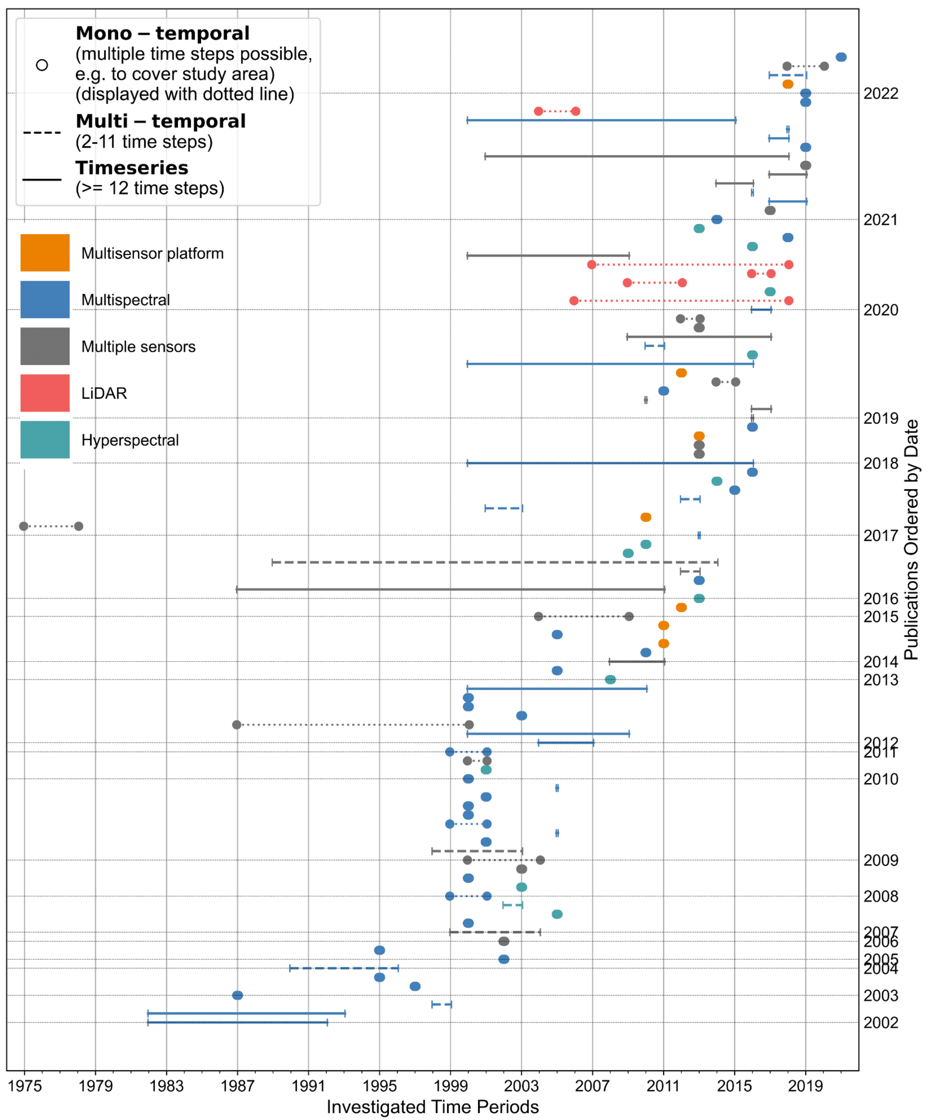
• The varying temporal periods of remote sensing data grouped by sensors, and the proportions of mono-temporal, multi-temporal and time-series approaches in field and remote sensing data are the focus of Section 3.4.
• As a final result, the thematic analysis (Section 3.5) covers the temporal distribution of spectral diversity concepts and presents the most frequently used spectral indices. In addition, the share of analyzed biodiversity scales ($\mathsf{\alpha }$, $\mathsf{\beta }$, and $\mathsf{\gamma }$ diversity), and focus on flora/fauna is presented.

3.1. General Information on the Research Interest over Time

As a general introduction to the number of studies per year classified in Web of Science categories (Table S2, Supplementary Materials), Figure 3 displays an increasing trend of the total number of publications per year from 2002 to 2022. With a maximum of 14 publications in 2021, the increasing popularity of spectral diversity as a remote sensing proxy for forest biodiversity is also highlighted by more than 10 publications each for the years 2019 to 2021. Overall, about 41% of the reviewed studies are categorized as “Environmental Sciences”, followed by a combination of “Environmental Sciences and Remote Sensing” (about 32%). Studies that have a strong focus on either “Ecology” (15%) or “Remote Sensing” (12%) present similar shares. Early studies (2003–2006) are solely classified as “Environmental Sciences”, whereas recent years present a greater mix of categories. In 2021 the combination of “Environmental Sciences and Remote Sensing” amounts to 8 publications, which is the second highest total number of a single category, only dominated by the year 2019 with 10 publications for “Environmental Sciences”. The increasing number of recent publications is underlined by the fact that more than 56% of all studies have been published since 2016, although the year 2022 did not end until the last access of the literature databases (26 August 2022). In other words, less than 44% of all studies have been published in about 2/3 of the investigated time period (2002 to 2015).

Figure 4 depicts the number of publications per publisher, journal, and most frequent first authors. Most studies are published in Wiley, with a total number of 25 publications (Figure 4b). Because Elsevier Science Inc., Elsevier, and Elsevier Science Bv. are defined as unique publishers in the Web of Science database, they have not been aggregated. When combined the total number amounts to 40 publications.

When aggregating all journals with a single publication (class “Others”), the total number amounts to 24 publications (Figure 4a). Interestingly, the journals with the second (Remote Sensing of Environment, Elsevier, 18 publications) and third highest number of publications (Remote Sensing, MDPI, 10 publications) both have a strong focus on remote sensing. The journals Ecological Applications (Wiley, 8 publications) and Ecological Indicators (Elsevier, 7 publications) come in fourth and fifth position, respectively.

The statistics about the number of publications in Figure 4c) based on the first author shows very different total numbers. About 15% of all reviewed articles (16 publications) are first authored by Duccio Rocchini (BIOME Lab, Department of Biological, Geological and Environmental Sciences, Alma Mater Studiorum University of Bologna, Bologna, Italy; Department of Spatial Sciences, Czech University of Life Sciences Prague, Faculty of Environmental Sciences, Praha, Czech Republic). Furthermore, there are 13 first authors with more than one publication, who together contribute by about 41% (45 publications) to all reviewed articles.

3.2. Spatial Analysis on Affiliations and Study Areas

The spatial analysis of the countries from the first author affiliations is depicted in Figure 5. Overall, the first authors included in this review come from 25 different countries. The country holding the most affiliations from first authors are the United States (24 publications), followed by Italy (21 publications). When aggregating all countries from the affiliations of first authors with a single publication, the total number amounts to 12 countries; Finland (8 publications), India (8 publications), and Germany (7 publications) present similar numbers of publications.

Almost half of all publications are from first author affiliations situated in Europe (44%). The proportion of publications from first author affiliations from the United States amounts to 27%, followed by Asia with 17%. Continents with a share of lower than 10% are South America (6%), Africa (5%), and Australia and Oceania (1%).

The spatial analysis of study areas is displayed in Figure 6. From all reviewed publications (n = 109), 105 studies are conducted at country level or smaller scale. Only four studies [62,83,84,85] are analyzing biodiversity based on spectral diversity from remote sensing at continental scale (Europe: three studies, North America: one study). Overall, most studies are from Europe (34 publications), followed by Asia and North America (both 25 publications). The countries of study areas holding more than 10 publications are India (12 publications) and the United States (15 publications). In Europe, Germany (7 publications) and Italy (9 publications) are the two countries with more than five publications each.

In addition to the spatial analysis of the study areas at country and continent level, study areas have been classified into four different forest types (tropical, subtropical, temperate, sub-frigid) according to the publication of Xu et al. 2022 [86]. Key climatic criteria for the classification of forest types are annual temperature and annual precipitation: tropical forests are characterized by annual temperatures greater than 20 °C and annual precipitation of greater than 2000 mm. Sub-tropical forests hold annual temperatures between 10 to 20 °C and annual precipitation in the range from 1200 to 2000 mm. In contrast, temperate forests present lower annual temperature (0 to 10 °C) and annual precipitation (800 to 1200 mm). Sub-frigid forests are characterized by lowest annual temperature (−5 to 0 °C) and annual precipitation (400 to 800 mm) [86].

Most studies are conducted in subtropical forests (40 publications), followed by tropical (38 publications) and temperate forests (30 publications). Therefore, more than 72% of all studies are focused on subtropical or tropical forests. Temperate forests hold a share of about 28%. From all reviewed studies, there is only one publication [87] that investigates biodiversity in sub-frigid forests based on remotely sensed spectral diversity.

When comparing the spatial analysis of the countries from first author affiliations with the countries of the study areas, strong discrepancies can be observed. At continental scale, the strongest differences are that only 6% of the first authors affiliations are from South America, although about 14% of all study areas are located in South America. Similarly, about 23% of all study sites are in Asia, but only a share of 17% of the first author affiliations are situated in Asia. At country level, Italy presents strong discrepancies since about 19% of all reviewed studies are from first authors with an affiliation in Italy, but only about 8% of the study sites are in Italy. Furthermore, there are opposing findings for Finland (eight first authors, one study area) and Peru (one first author, eight study areas). Overall, in 57.8% of all reviewed articles the country of the first author’s affiliation is equal to the investigated country.

3.3. Analysis on Remote Sensing Sensors

The analysis of spectral diversity from remote sensing sensors in the reviewed articles shows a wide range of sensors that have been used (Figure 7). In general, the different sensors can be categorized into active (LiDAR, SAR, topographic radar) and passive sensors (multispectral, hyperspectral). In comparison to active sensors, passive remote sensing sensors do not have their own energy source, i.e., they do not emit radiation. Moreover, passive sensors are measuring solar radiation that has been reflected by objects on the Earth’s surface, e.g., vegetation. The measured radiation is commonly detected in band lengths ranging from the visible light to shortwave infrared. In addition, passive sensors are specifically sensitive to atmospheric effects (e.g., clouds, haze), whereas active sensors emit radiation which is measured again once returned from an object. Active radar sensors which are most commonly operating in X- (2.5 to 3.75 cm wavelength), C- (5.43 to 5.66 cm wavelength), L- (20 to 60 cm wavelength), and P-band (60 to 120 cm wavelength) are rather insensitive towards atmospheric influences. In contrast, LiDAR sensors which are often emitting green or near-infrared light can not penetrate clouds [88,89,90].

From all sensors used in the reviewed studies, about 70% are multispectral remote sensing sensors from which spectral metrics have been generated for the analysis of forest biodiversity based on spectral diversity concepts. Hyperspectral sensors hold a share of about 10%, followed by LiDAR (9.7%). Overall, more than 80% of all the sensors used are passive remote sensing sensors highlighting the focus on optical diversity to estimate forest biodiversity. The least commonly used sensors are topographic radar (5.5%), multisensor platforms (3.4%; airborne platform that consists of combinations of multispectral, hyperspectral, and LiDAR sensors which are operating simultaneously), and SAR sensors (1.4%).

The most frequently used sensor is Landsat 7 which was integrated in 24 publications, although data gaps occurred since 2003 because of errors with the scan line corrector [91,92]. Other commonly used passive sensors are Sentinel-2 (15 publications), Landsat 8 (13 publications), Moderate-resolution Imaging Spectroradiometer (MODIS, 13 publications), and Landsat 5 (11 publications). The statistics highlight the applicability of the continuous time-series from sensors of the Landsat mission (NASA, 1972 to today) since the total number of publications amounts to 49 publications, i.e., about 34% of the total number of remote sensing sensors used (n = 145) are from the Landsat mission. The class “ALS” (airborne laser scanning) aggregates different airborne LiDAR sensors and is the most commonly used non-optical sensor type (11 publications). In contrast, the total number of integrated SAR sensors (Sentinel-1, AIRSAR) in the reviewed articles amounts to two publications.

To better understand the contribution of airborne and satellite remote sensing, but also of field work for validation of remotely sensed products, Figure 8 provides an overview on the spatial scales and spatial resolutions. In more than 80 studies, satellite remote sensing (n = 85) and field work data (n = 94) were obtained. Therefore, in only 15 studies the airborne or spaceborne remotely sensed products were not validated by field data. Airborne remote sensing data were integrated in 33 reviewed articles.

The analysis on the spatial resolution of remote sensing data highlights that there are two major spatial resolutions preferred for investigating forest biodiversity using spectral diversity concepts: very high (≤5 m, 46 publications) and medium spatial resolution data ($10-\le$30 m, 58 publications). Very high spatial resolution remote sensing data comprises, for example, airborne laser scanning data, AVIRIS hyperspectral imagery, or multispectral sensors such as Quickbird, RapidEye, IKONOS or WorldView-2. The group of medium spatial resolution sensors mainly consists of Landsat 5, 7 and 8. High (21 publications, e.g., Sentinel-2) or coarse spatial resolution sensor (19 publications, e.g., MODIS) are less frequently integrated in the reviewed studies.

3.4. Temporal Analysis on Remote Sensing and Field Data

In the following, the temporal periods of remote sensing data per reviewed article are analyzed. Furthermore, the different temporal scales of field (mono-temporal, bi-temporal) and remote sensing data (mono-temporal, multi-temporal, time series) are explained.

Figure 9 depicts the investigated time period of the remote sensing data in comparison to the publication dates of the reviewed articles. Per study, the remote sensing data are categorized into the classes hyperspectral imagery, LiDAR observations, data from multiple sensors (combination of different remote sensing sensors in a study), multispectral imagery, or data from a multisensor platform (simultaneous acquisition of different remote sensing sensors from a single airborne platform). The time periods of remote sensing data are grouped into mono-temporal (one time step), multi-temporal (two to 11 time steps monitored), and time series approaches (more than 12 time steps monitored). It is important to note that the remotely sensed data of some studies are actually a composite of multi-temporal imagery, e.g., to cover the complete study area. Since the scenes of the composite are treated as mono-temporal imagery, i.e., no analytical comparisons are made between the acquisition dates, those remote sensing data sets are classified as mono-temporal approach. Since there was no information about the temporal period of the remote sensing data in the original article or the Supplementary Material of the study by Chi et al. 2019 [93], this study could not be included in the temporal analysis.

Overall, there are great benefits of multi-temporal or time series remote sensing approaches, since long term dynamics can be monitored and changes can be identified [42]. With the opening of the Landsat archive in 2008, the freely available continuous time series from Landsat 1 to nowadays Landsat 9 enables tracking changes of land surface dynamics at a novel temporal scale [94]. In addition, the launch of the Sentinel satellites from ESA (e.g., Sentinel-1 in 2014 and Sentinel-2 in 2015) [95,96] complements the imagery derived from Landsat and offers the generation of fusion products. Therefore, harmonized high temporal resolution data sets of surface reflectance information can be generated based on the combined multispectral sensors from Landsat and Sentinel-2 [41].

Figure 9 shows that all time series analysis of the reviewed articles are based on spaceborne multispectral sensors (about 13%) or multiple sensors (combination of multispectral sensors and others, about 9%). Early multispectral time series approaches were published by Oindo 2002 [97] and Oindo & Skidmore 2002 [77] based on AVHRR data to investigate the species richness in Kenya. Since the year 2009, more and more studies integrated remote sensing time series data for the analysis of forest biodiversity using spectral diversity concepts [54,62,85,98,99,100,101,102,103,104,105,106,107,108,109,110,111,112,113,114,115,116]. Studies that are solely based on LiDAR data have become specifically popular since the year 2020: on the one hand, all studies are based on mono-temporal remote sensing data, and on the other hand, the LiDAR data was derived from an airborne sensor [79,117,118,119,120]. Another finding is that studies integrating multiple sensors have greatly increased in recent years: more than 55% of all reviewed studies based on remote sensing data from multiple sensors have been published since 2018 [54,105,106,107,109,113,114,121,122,123,124,125,126,127].

To better understand the different temporal scales of field and remote sensing data, Figure 10 provides an overview on the contribution rates. About two thirds of all reviewed studies (66%) integrate mono-temporal remote sensing data. Aforementioned time series approaches only amount to about 22%, and the smallest share (12%) hold multi-temporal studies. In comparison, the proportion of mono-temporal field data to validate remotely sensed products makes up 84% of all reviewed studies. In 15% of all reviewed articles no field data was collected. The collection of bi-temporal field data only amounts to a minor fraction of 1% and highlights the challenges that come along with the bi-temporal field sampling which was stressed extensively in the early studies of Palmer 1995 [34] and Palmer et al. 2002 [35].

3.5. Review of Thematic Foci

In the following, the results of a thematic analysis are presented in separate sections covering the temporal development of the three spectral diversity concepts (Section 3.5.1), modelling responses (biodiversity scales) and environmental foci (flora/fauna) (Section 3.5.2), and spectral indices used as a measure of forest richness and heterogeneity (Section 3.5.3).

3.5.1. Comparison of the Different Spectral Diversity Concepts: Vegetation Indices, Spectral Information Content, and Spectral Species

Spectral Diversity is not an isolated concept of remote sensing to monitor biodiversity. Moreover, different approaches such as habitat mapping, species mapping or functional diversity estimation can be combined with spectral diversity methods for a comprehensive picture of biodiversity [51] (Table 2). In the introduction of this review in Section 1.2, a brief overview on the different concepts of spectral diversity was given according to Wang & Gamon 2019, namely vegetation indices, spectral information content, and spectral species. In the following, those concepts are presented more in detail by highlighting exemplary studies.

The calculation of vegetation indices is an essential part of optical remote sensing to generate spectral proxies that are specifically sensitive towards the object of interest or the investigated phenomena. The pixel-based estimation of optical vegetation indices can be classified according to the combined spectral wavelengths [40]. As an early spectral diversity concept, spatial and temporal variation of vegetation indices (e.g., mean or standard deviation of NDVI) was assessed and linked to field plot measurements of biodiversity. The calculated spectral variation based on a vegetation index is defined as a spectral diversity index which can be related to taxonomic, functional, and genetic diversity [51]. More than 79% of the reviewed studies based on spectral diversity from vegetation indices are based on multispectral imagery [44,54,72,83,87,93,103,107,123,128,129,130,131,132,133,134,135,136,137], while about 74% of those studies are integrating data from Landsat sensors [44,54,72,87,93,103,107,128,129,132,133,134,135,136].

The second concept of spectral diversity is called spectral information content [51]. Spectral diversity analysis based on spectral information content can be grouped into metrics based on information theory in original and transformed spectral space: an example of the original spectral space is the calculation of the coefficient of variation from NDVI [77,97], whereas transformed spectral space refers for example to ordination methods such as the convex hull volume in principal component analysis (PCA) space [73]. From all reviewed studies that analyze forest biodiversity based on spectral diversity from spectral information content, more than 78% of those studies are based on multispectral imagery. Furthermore, about 51% of aforementioned studies integrated Landsat data, while only about 19% obtained Sentinel-2 data for their analysis.

The spectral species concept was introduced by Féret & Asner 2014 [55] linking taxonomic species and remotely sensed spectral species in an unsupervised classification approach. Based on airborne hyperspectral imagery, estimates of $\mathsf{\alpha }$ (Shannon diversity) and $\mathsf{\beta }$ diversity (Bray–Curtis dissimilarity) are derived from a workflow combining ordination techniques (PCA) and k-means clustering. To compress the high-dimensional spectral data from airborne imaging spectroscopy, PCA and subsequent feature selection are applied, followed by the definition of spectral species using the k-means clustering algorithm. In an iterative process, maps of $\mathsf{\alpha }$ and $\mathsf{\beta }$ diversity (projection in RGB space using nonmetric multidimensional scaling, NMDS) are generated to identify richness in local communities and gradients of different species compositions [55,81,138]. Initially, the spectral species concept was developed based on high spatial resolution hyperspectral imagery to match the increased variability, species richness and spectral similarity of species in tropical forests [55,138,139]. In recent studies, the spectral species concept was applied to other forest types and different remote sensing sensors, such as Sentinel-2 [140,141,142] or MODIS [85]. As an example, the study of Gastauer et al. 2022 [142] applied the spectral species concept in Eastern Amazon, Brazil, to monitor forest regeneration in an iron mining complex using Sentinel-2 imagery and bi-temporal field sampling of vegetation and soil characteristics.

The temporal distribution of all reviewed articles on spectral diversity grouped by the three concepts vegetation indices, spectral information content, and spectral species is depicted in Figure 11. Overall, there are 24 publications on vegetation indices (22.0%) [44,53,54,72,74,83,87,93,103,107,119,123,128,129,130,131,132,133,134,135,136,137,143,144], 76 reviewed articles on spectral information content (69.7%) [45,46,56,58,59,60,61,62,73,76,77,79,80,82,84,97,98,99,100,101,102,104,105,106,108,109,110,111,112,113,114,115,116,117,118,120,121,122,124,125,126,127,145,146,147,148,149,150,151,152,153,154,155,156,157,158,159,160,161,162,163,164,165,166,167,168,169,170,171,172,173,174,175,176,177,178], and 9 studies about the spectral species concept (8.3%) [55,75,85,138,140,141,142,179,180]. From 2002 to 2013 there are only studies based on vegetation indices or spectral information content. With the publication of the spectral species concept in 2014 [55,138], there were additional studies in 2016 [75], 2019 [179,180], 2020 [141], 2021 [85,140], and 2022 [142]. Especially since 2017 there was an increasing number of reviewed studies using spectral information content to assess forest biodiversity, contributing by over 55% to all studies about spectral information content. When referring to the aforementioned studies (n = 42), the ratio of Landsat based studies (about 29%) compared to studies integrating Sentinel-2 data (about 26%) is much closer since there was the launch of Sentinel-2B in 2017 (Sentinel-2A was launched in 2015).

Sensors from the Landsat mission, Sentinel-2, and MODIS are the most frequently used sensors in the reviewed articles (Figure 7). When grouping those sensors by spectral diversity concept, there are strong differences: about 58% of all studies based on vegetation indices are integrating Landsat data (14 publications), while there are only about 4% based on Sentinel-2 or MODIS data respectively (one study each). Studies based on spectral information content hold a share of 39% for Landsat data (30 studies), 14% for Sentinel-2 (11 studies), and 14% for MODIS (11 studies). From the nine studies about spectral species, none of them are based on Landsat data, three studies are integrating Sentinel-2 data [140,141,142], and there is one study using MODIS data [85]. From all reviewed studies, there are only two studies combining Sentinel-2 and Landsat data: Farwell et al. 2021 [54] (vegetation indices) and Torresani et al. 2019 [106] (spectral information content). The study of Silveira et al. 2021 [114] is the only study combining MODIS and Landsat data (spectral information content).

3.5.2. Model Responses and Environmental Foci

Figure 12 depicts the number of publications for different biodiversity scales ($\mathsf{\alpha }$, $\mathsf{\beta }$, and $\mathsf{\gamma }$ diversity) and environmental foci (flora, fauna). Most of the studies are analyzing $\mathsf{\alpha }$ diversity (93 publications), followed by $\mathsf{\beta }$ diversity (50 publications). There are 34 studies that conducted a combined analysis of $\mathsf{\alpha }$ and $\mathsf{\beta }$ diversity. Landscape biodiversity ($\mathsf{\gamma }$ diversity) is explicitly estimated in only two studies [117,127]. The analysis on environmental foci reveals that the majority (92.7%) of all reviewed studies analyzed floristic information to assess forest biodiversity. Only a small number of studies solely investigated fauna data (4.6%), and less than 3% of all reviewed studies conducted a combined analysis of flora and fauna. Most floristic studies estimated tree species diversity, e.g., [44,75,106,129,148,149,157], as a proxy of forest biodiversity. In contrast, some studies sampled understory vegetation (e.g., pterophytes) which are used as proxies for local tree species diversity since canopy building tree species are more challenging to identify [59,149,173].

3.5.3. Spectral Indices for the Analysis of Optical Diversity

Since the majority of reviewed articles integrated optical imagery from which spectral indices can be calculated, the following paragraph focuses on the different spectral indices used. Based on all reviewed studies using optical imagery (n = 103), 28 studies did not use spectral indices, while 75 studies calculated spectral indices (Figure 13a). In total, 58 different spectral indices have been calculated. Moreover, the proportion from all reviewed articles integrating spectral indices that were used at least twice amounts to about 76%. Those most commonly used spectral indices were classified according to Zeng et al. 2022 [40] (Figure 13b) to better understand the contribution rates of different wavelength ranges.

When focusing on the classified wavelength classes (Figure 13b, inner circle), spectral indices in the red to near-infrared (NIR) make up about 71%. All other categories hold shares lower than 10%, with spectral indices in the visible to NIR holding the highest share (about 9%) of this group. The NDVI is the most commonly used spectral index in the reviewed articles (56.7%), followed by the Enhanced vegetation index (EVI, 8.7%) being the only spectral index in the visible to NIR.

The applications of NDVI range from the analysis of spatial patterns, over temporal variability, to the correlation of NDVI with other spectral indices or remotely sensed proxies of forest biodiversity. Statistical relationships of spatial patterns in NDVI with in situ measurements of species richness were found in the Western Ghats, India based on multispectral imagery from Resourcesat-1 LISS-III [107,130], and other biodiversity hotspots in India (Himalaya, Indo-Burma) using Landsat 5 data [107]. Studies on the tropical forests in Florida, United States [72,132] also highlighted the applicability of spatial statistics of mean NDVI to explain tree species richness, but identified heterogeneity metrics (standard deviation of NDVI) to be less suited for the forests of Florida due to low disturbance rates. Furthermore, NDVI was significantly correlated with stand density [72]. The study of Parviainen et al. 2009 [135] also stressed the applicability of NDVI derived metrics to explain local and landscape species richness in boreal forests of Finland.

The analysis on the influence of biotic (e.g., forest productivity estimated by NDVI) and abiotic factors on species richness in Hawaiian dry forests by Pau et al. 2012 [101] found out that there is no direct effect of multi-temporal NDVI on species richness. Other studies [46,54,98,131,158] also identified challenges and variability with NDVI to understand temporal patterns in species richness. He et al. 2009 (analysis of plant species diversity) and Ribeiro et al. 2019 (analysis of bird species diversity) both suggested the applicability of summer NDVI (vegetation growth maximum) for the correlation with species richness. Limitations of NDVI are discussed in several studies because of saturation effects in dense forests [54,130,153]. To overcome those limitations, multiple studies proposed additional spectral indices for the assessment of biodiversity in dense, high biomass forests, such as first and second order texture metrics based on EVI [54], the combination of multiple spectral indices and metrics (e.g., DVI (Difference vegetation index), EVI (Enhanced vegetation index), NDVI, VARI (Visible atmospherically resistant index), WDRVI (Wide dynamic range vegetation index) and tasseled cap features, mean reflectance statistics, land surface temperature) [100,103,114].

To investigate the capability of SAR data to explain tree species richness, Gillespie et al. 2009 [44] compared Landsat 7 derived NDVI with VV (vertical transmit, vertical receive) polarization from C- and L-band airborne SAR (AIRSAR) metrics. The authors found out that mean statistics are reaching higher correlations than statistics based on standard deviation for both NDVI and SAR metrics. In addition, combined metrics of C- and L-band SAR data could explain slightly more variance (50% variance explained) than NDVI metrics (41% variance explained).

Multiple studies used NDVI as input metrics to calculate spectral $\mathsf{\alpha }$ and $\mathsf{\beta }$ diversity (e.g., spectral Shannon index, spectral Simpson index, Rao’s Q index [181,182], spectral information content) [62,83,84,85,99,108,115,116,121,124,126,157,159,167,170].

The findings based on NDVI statistics correlated with forest biodiversity metrics suggest the combined analysis of NDVI with additional spectral indices. Furthermore, Rao’s Q index has been proposed as an improved spectral estimate for the calculation of $\mathsf{\alpha }$ diversity and $\mathsf{\beta }$ diversity (spatial statistics using moving window approaches) because it combines in its calculating the relative abundance and pair-wise distance of spectra derived from an input metrics (e.g., NDVI) compared to spectral Shannon index which does not consider the numerical magnitude of spectral values [79,84,115,116,124]. Further benefits of Rao’s Q index are that multidimensional input metrics can be integrated, e.g., a stack of various spectral indices for a more comprehensive characterization of vegetation condition [84].

4. Discussion

4.1. Overall Discussion on the Validity of the Spectral Variation Hypothesis

An overall discussion on the validity of the SVH was introduced by several studies that noted spatial scale dependencies, temporal effects, ecosystem biases, and influences from the remotely sensed spectral diversity metrics and in situ measurement of biodiversity on the analysis of forest biodiversity using spectral diversity concepts [51,60,61,74,153,162,163,168]. Many of those effects need to be considered in any analysis based on remote sensing data, and are not only relevant for forest biodiversity estimation from remotely sensed spectral diversity [61].

The influence of spatial resolution from remote sensing imagery on the capability to detect a certain object or phenomena is well-known since a target of research can only be identified if the pixel size of remote sensing data is at least the size or smaller than the object [36,90]. Since forest biodiversity is a multifaceted phenomena of taxonomic, functional, and structural diversity, there is not a single adequate spatial scale to identify a direct relationship [99,121,153]. Moreover the concept of spectral diversity hypothesizes an indirect, more generic link between heterogeneity in the remotely sensed signal and forest biodiversity, compared to direct approaches of forest biodiversity assessment such as habitat and species mapping [51,61]. Fassnacht et al. 2022 [61] highlighted the challenge of the SVH to differentiate between the original SVH (spectral variation as a proxy of habitats or vegetation types) and the species SVH (spectral variation from very high spatial resolution imagery as a proxy of species). Besides the spatial resolution of the sensor, also the sampling design and grain size of field plots influence the relationship of remotely sensed spectral diversity with forest biodiversity [51,130,131]. Overall, there are different findings of studies testing sensors with varying spatial resolutions: Nagendra et al. 2010 [134] found that an increased spatial resolution of IKONOS data is not necessarily beneficial since it comes along with shading effects and lower spectral resolution compared to publicly available Landsat data. Rocchini et al. 2007 [162] suggested a distance decay approach to estimate environmental gradients solely based on near infrared information from higher spatial resolution imagery since mixed pixel effects might be reduced which is an opposing finding to Nagendra et al. 2010 [134]. Similarly, Rocchini et al. 2004 [78] noted that higher spatial resolution sensors can result in increased correlation of spectral heterogeneity and species diversity which is aligned with the findings of higher correlations of Rao’s Q index based on NDVI using Sentinel-2 (10 m) compared to Landsat data (30 m) in an alpine coniferous forest [106].

Besides spatial scale effects, the radiometric resolution plays an important part in the delineation of different tree species. The study of Ferreira et al. 2016 [148] emphasized the importance of the short wave infrared (SWIR) band since tree species discrimination based on simulated WorldView-3 imagery benefited from additional bands in the longer optical wavelengths. The trade-off of high spatial resolution and lower spectral resolution was also discussed in other studies suggesting the combined use of e.g., Landsat, Sentinel-2 and WorldView imagery to test the influence of different sensor characteristics [121,128].

Since previous results of the temporal periods of remote sensing data present a dominating proportion of mono-temporal approaches (about 66%, Figure 10), it is important to note that those studies are analyzing a static picture of a phenological snapshot. Aforementioned sensitivity of the SVH towards temporal periods (e.g., phenological status of vegetation), was a research focus of several studies integrating multi-temporal or time series remote sensing data to test changes in spectral diversity at different phenological stages [46,100,101,103,108,109,121,143,157], estimate long-term changes in ecosystem stability [97], identify areas for protection and conservation management (biodiversity hotspots) [114], monitor regeneration after disturbance [142], or aggregate time series remote sensing data to have a more reliable estimate of an overall vegetation condition [54,107].

The species diversity estimate derived from in situ measurements is an important influence on the relationship between spectral diversity and forest biodiversity [61]. In the reviewed studies, a wide range of forest biodiversity estimates was assessed with a major proportion (92.7%) focusing on floristic characteristics (Figure 12). Biodiversity estimates from vegetation can be grouped into community inventory [131], tree species diversity [45,80,100,177], vascular plant species [162,164,166], and understory vegetation [59,149,173]. Forest biodiversity proxies based on animal data comprise multidiversity estimates (birds, bats, and others) [105,119], bird species richness data [46,54], tick abundance information [82], behavioural data of redtail monkeys [136], and mammal and herbivore inventory [77,97].

Spectral diversity metrics to assess forest heterogeneity cover different statistics based on spectral indices (mean, standard deviation, coefficient of variation) [77,97,107,130,131], texture metrics based on spectral indices [46,54,110,114,125], heterogeneity/diversity indices adapted to remote sensing (spectral Shannon and Simpson index, Rao’s Q index) [79,84,115,116,124], metrics derived from self-organizing feature maps [80], and estimates based on the spectral species concept [55,75,85,138,140,142,179,180].

4.2. Benefits and Limitations of the Three Spectral Diversity Concepts

Based on spectral diversity from vegetation indices, spectral information content, and spectral species, an estimate of forest biodiversity can be derived. A general limitation of vegetation indices are that those can only be calculated from optical sensors (optical diversity), while spectral information content or spectral species metrics derived from optical sensors can be supplemented by complementary metrics on forest biodiversity (e.g., LiDAR based forest structure metrics) which might better assess overall forest biodiversity characteristics than single estimates of vegetation indices [44,45,46,79,81,105,117,118,119,120,122,149,171]. Nevertheless, the wide wavelength range covered by spectroscopic sensors (multispectral, hyperspectral) and comprehensive stacks of derived vegetation indices and band statistics are valuable input metrics for the calculation of spectral information content (e.g., PCA based on spectral indices) [159] and spectral species (e.g., Sentinel-2 based analysis) [140,141,142].

Compared to vegetation indices and spectral information content, the spectral species concept analyzes species diversity based on a globally collected spectra (complete scene analyzed) which is clustered into a defined number of spectral species. In contrast, the estimation of spectral diversity from vegetation indices and spectral information content is calculated locally (local or focal operation), i.e., there is no consideration of a global spectral distribution when spectral heterogeneity is estimated [55]. The calculation of forest biodiversity from spectral information content or spectral species is influenced by the intra-class spectral variation since large within-class variations can lead to a subdivision of taxonomic species into, for example, multiple separate spectral species. In general, there is an ongoing discussion on the entity of a spectral species since local spectral species might be generalized to global spectral communities when coarsening the spatial resolution [85]. On the other hand, the assignment of spectral species benefits from the clustering of e.g., atmospheric artefacts or background conditions as separate spectral species, while spectral diversity based on vegetation indices or spectral information content might be more sensitive towards those influences.

Overall, Féret & Asner 2014 [55] highlighted benefits in accuracy when calculating $\mathsf{\alpha }$ and $\mathsf{\beta }$ diversity in forests based on the spectral species concept compared to estimates from vegetation indices or spectral information content. Correlation statistics of $\mathsf{\alpha }$ diversity from field measurements (Shannon index) and local diversity calculated based on spectral species resulted in highly significant correlations (p < 0.001, r = 0.86). The analysis of spectral information content using the mean distance from the spectral centroid (p < 0.05, r = 0.26), and variation in NDVI as estimate of spectral diversity from vegetation indices reached lower accuracies (p > 0.05, r = 0.06).

4.3. Future Research Directions

With the advance of remote sensing for biodiversity monitoring, global initiatives such as the Group on Earth Observations Biodiversity Observation Network (GEO BON), the Committee on Earth Observation Systems (CEOS) Biodiversity task, and the International Geosphere Biosphere Programme (IGBP), have formed and strongly promote, among others, the future capabilities of species diversity assessment based on earth observation data to investigate the drivers of global change [183,184]. Recently, Skidmore et al. 2021 published an updated list of essential biophysical variables (EBVs) and categorized remote sensing biodiversity products into ranked EBV classes for a more consistent framework of biodiversity monitoring [185].

Forest biodiversity analysis is related to various fields of research. An exemplary list are the identification of biological corridors [128], disease biogeography [82], analysis on the impact of non-natural disturbances on forest regeneration [80,142], comprehensive ecosystem understanding based on multidiversity data [105,119], identification of environmental gradients using beta diversity information [170], and novel approaches correlating spectral and taxonomic species for an increased understanding of spectral species and communities [55,81,85].

The progress of remote sensing based on multi-scale and complementary sensors in forest-related research is facilitated by open-code and open-data policies (shared code [45,56,84,105], programming packages [141,186], data availability [94,95]). The ongoing operation of multiple spaceborne high-resolution optical sensors (Sentinel-2A and -2B, Landsat 8, Landsat 9) offer great resources for large-scale forest biodiversity monitoring at improved temporal scales [41,42]. Furthermore, the recent launch of EnMAP (1 April 2022, [187]) will provide global hyperspectral imagery complemented by data of other hyperspectral missions such as PRISMA [188]. Forest structure information derived from GEDI for all tropical and temperate forests adds further value to the analysis of forest biodiversity since there are various data sets on biomass, vertical and horizontal canopy structure, and foliage complexity derived from the full waveform LiDAR [189,190]. With the extension of the SVH on LiDAR data (HVH, [79]), the concept could be further expanded by the integration of structural information derived from SAR data, e.g., Sentinel-1 and upcoming missions (BIOMASS: P-band [191], NISAR: L- and S-band [192]). Overall, the combination of research at multiple spatial scales (terrestrial, drones, airborne, spaceborne) using remote sensing enables the understanding of biodiversity phenomena at larger-scale with observations at multiple time steps from spaceborne sensors where field work reaches its limitations [34,35,57]. Furthermore, bridging disciplines of remote sensing, ecology, and environmental sciences will improve the overall understanding of forest biodiversity and create more trans-disciplinary research networks.

5. Conclusions

This review provides an overview on forest biodiversity monitoring using remotely sensed spectral diversity concepts. In total 109 studies were analyzed to collect information on the spatiotemporal distribution of the reviewed articles, airborne and spaceborne sensors used in the analysis, temporal periods of remote sensing and field work data, and thematic foci. The thematic analysis covers the temporal distribution and characteristics of the three spectral diversity concepts, spectral indices derived from optical sensors, and biodiversity scales. In the following, the main findings are summarized:

• In recent years there was an increasing number of studies on forest biodiversity monitoring from remotely sensed spectral diversity. Since 2016, more than 56% of all studies were published which underlines the increasing relevance of forest-related research in the context of climate change.
• Several research hotspots were identified with most studies investigating forest biodiversity in the United States and India. Grouped by continent, about one third is focusing on European forests, followed by Asia and North America (each continent holds about one fourth). Overall, there is a strong focus on temperate, sub-tropical and tropical forests, while other forest types (e.g., sub-frigid) are only investigated in a single study. Strong discrepancies between the country of the first author affiliation and the country or continent under study were identified: at continental scale, the strongest discrepancy is found for South America which holds a share of about 6% of all first authors and about 14% of all study sites. At country level, about 19% of the affiliations of first authors are in Italy, while only about 8% of all studies are investigating forest biodiversity in Italy.
• Research on forest biodiversity based on remotely sensed spectral diversity derived from vegetation indices, spectral information content and spectral species has a strong focus on optical sensors. About 70% of all reviewed articles are integrating multispectral imagery, and about 10% are based on hyperspectral data. Most commonly used multispectral sensors are Landsat 7 (24 applications), Sentinel-2 (15 applications), Landsat 8 (13 publications), MODIS (13 publications), and Landsat 5 (11 publications).
• Most studies are integrating data from field work as estimate of in situ biodiversity (94 articles). Remotely sensed spectral diversity is dominantly assessed using spaceborne sensors (85 applications), while data from airborne sensors are applied in 33 reviewed articles. Furthermore, there is a tendency towards the integration of very high (≤5 m, 46 applications) on the one hand, and medium spatial resolution imagery ($10-\le$30 m, 58 publications) on the other hand.
• The analysis of temporal scales of remote sensing and field data present a strong focus on mono-temporal resolution. About 66% of all remote sensing data are from one time step, while multi-temporal (about 12%) and time series approaches (about 22%) hold much lower shares. Overall, all time series approaches are either based on multispectral imagery (about 13%) or data from multiple sensors (about 9%). Mono-temporal data from field work amount to 84%, 15% of all reviewed articles did not use field data, and only a minor proportion of about 1% collected bi-temporal in situ measurements of forest biodiversity.
• The comparative statistics of spectral diversity concepts show that most reviewed articles are based on spectral information content (about 70%), followed by vegetation indices (about 22%), and spectral species (about 8%). It is important to note that the spectral species concept was introduced in 2014, whereas articles based on vegetation indices or spectral information content were published since 2002. The promising findings on forest biodiversity using spectral species are highlighted by the adaption of the original concept using airborne hyperspectral data towards Sentinel-2 and MODIS data.
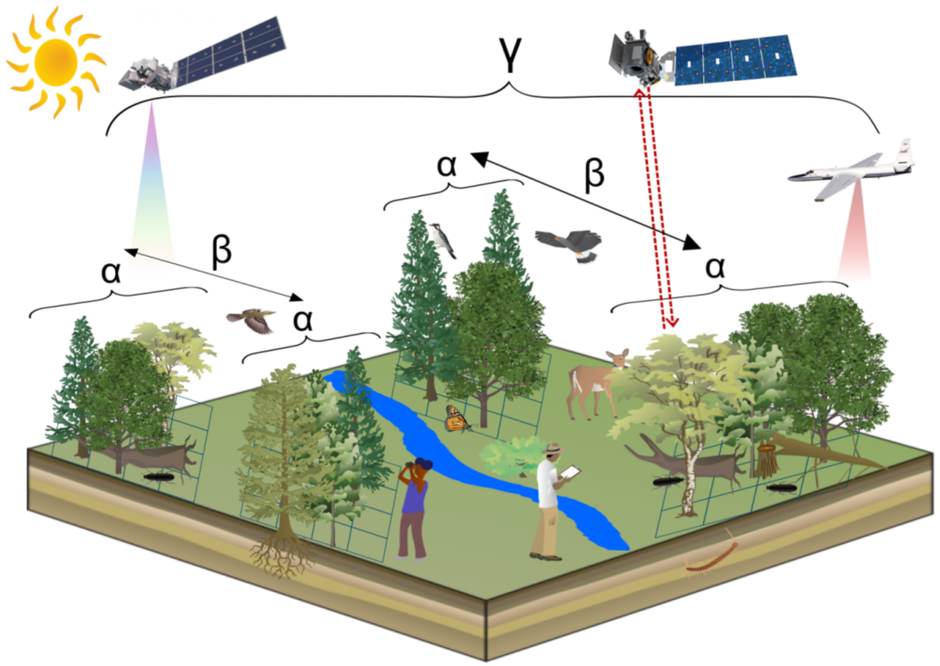
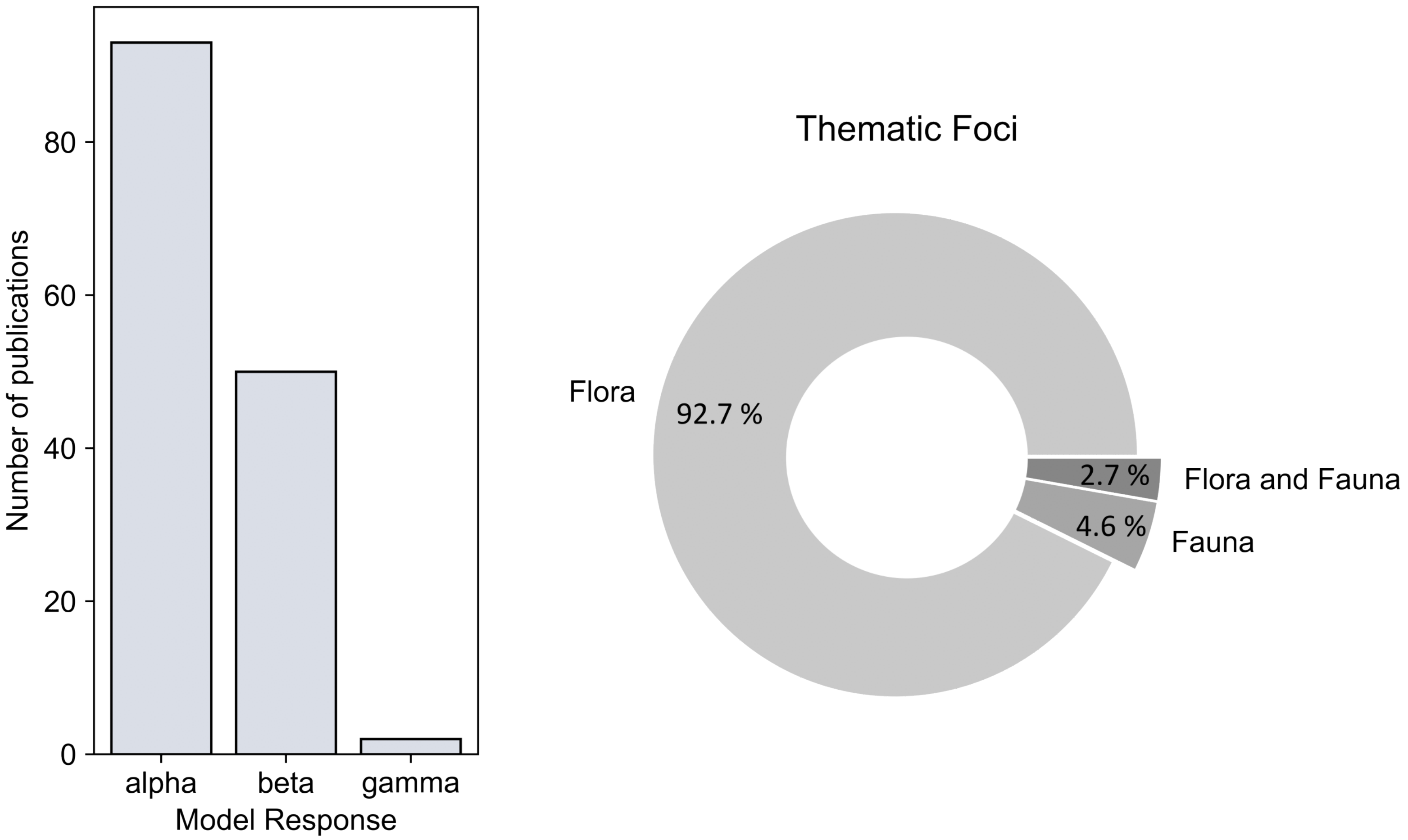
• Forest biodiversity was assessed at multiple scales: $\mathsf{\alpha }$, $\mathsf{\beta }$, and $\mathsf{\gamma }$ diversity. Most of the articles (n = 93) analyzed $\mathsf{\alpha }$ diversity, followed by 50 articles on $\mathsf{\beta }$ diversity, and a combined analysis of $\mathsf{\alpha }$ and $\mathsf{\beta }$ diversity in 34 articles. An explicit estimate of $\mathsf{\gamma }$ diversity was only calculated in two studies. The analysis on floristic characteristics as in situ biodiversity measure amounts to more than 92%, while analysis solely on fauna (about 5%), and combined analysis on flora and fauna (less than 3%) hold much lower shares.
• Many studies integrating optical imagery (n = 103) calculated spectral indices (n = 75). About 71% of those studies calculated spectral indices based on red to near-infrared bands. The most often used spectral index is the NDVI (about 57%), followed by the EVI (about 9%).

To summarize, this review presents a comprehensive analysis on forest biodiversity based on spectral diversity from airborne and spaceborne remote sensing. Notable progress was made regarding the development of statistical concepts and the growing number of complementary sensors integrated. Future efforts on the multi-temporal monitoring of forest biodiversity based on spectral diversity are necessary to complement findings on EBVs from change detection analysis.

References

1. Wilson, E.O. Biodiversity; National Academies Press: Washington, DC, USA, 1988. [Google Scholar]
2. Gaston, K.J. Global patterns in biodiversity. Nature 2000, 405, 220–227. [Google Scholar] [CrossRef] [PubMed]
3. Maclaurin, J.; Sterelny, K. What is biodiversity? In What Is Biodiversity? University of Chicago Press: Chicago, IL, USA, 2008. [Google Scholar]
4. Mittermeier, R.A.; Turner, W.R.; Larsen, F.W.; Brooks, T.M.; Gascon, C. Global Biodiversity Conservation: The Critical Role of Hotspots. In Biodiversity Hotspots; Springer: Berlin/Heidelberg, Germany, 2011; pp. 3–22. [Google Scholar] [CrossRef]
5. Reid, W.V. Biodiversity hotspots. Trends Ecol. Evol. 1998, 13, 275–280. [Google Scholar] [CrossRef]
6. Steffen, W.; Richardson, K.; Rockström, J.; Cornell, S.E.; Fetzer, I.; Bennett, E.M.; Biggs, R.; Carpenter, S.R.; de Vries, W.; de Wit, C.A.; et al. Planetary boundaries: Guiding human development on a changing planet. Science 2015, 347, 1259855. [Google Scholar] [CrossRef] [PubMed] [Green Version]
7. Barnosky, A.D.; Matzke, N.; Tomiya, S.; Wogan, G.O.U.; Swartz, B.; Quental, T.B.; Marshall, C.; McGuire, J.L.; Lindsey, E.L.; Maguire, K.C.; et al. Has the Earth’s sixth mass extinction already arrived? Nature 2011, 471, 51–57. [Google Scholar] [CrossRef] [PubMed]
8. Ceballos, G.; Ehrlich, P.R.; Dirzo, R. Biological annihilation via the ongoing sixth mass extinction signaled by vertebrate population losses and declines. Proc. Natl. Acad. Sci. USA 2017, 114, E6089–E6096. [Google Scholar] [CrossRef] [PubMed] [Green Version]
9. Dirzo, R.; Young, H.S.; Galetti, M.; Ceballos, G.; Isaac, N.J.; Collen, B. Defaunation in the Anthropocene. Science 2014, 345, 401–406. [Google Scholar] [CrossRef]
10. Almond, R.E.; Grooten, M.; Peterson, T. Living Planet Report 2020-Bending the Curve of Biodiversity Loss; World Wildlife Fund: Washington, DC, USA, 2020. [Google Scholar]
11. Betts, M.G.; Wolf, C.; Ripple, W.J.; Phalan, B.; Millers, K.A.; Duarte, A.; Butchart, S.H.M.; Levi, T. Global forest loss disproportionately erodes biodiversity in intact landscapes. Nature 2017, 547, 441–444. [Google Scholar] [CrossRef]
12. IUCN. The IUCN Red List of Threatened Species. Version 2022-1. 2022. Available online: https://www.iucnredlist.org (accessed on 9 May 2022).
13. Jones, J.P.; Collen, B.; Atkinson, G.; Baxter, P.W.; Bubb, P.; Illian, J.B.; Katzner, T.E.; Keane, A.; Loh, J.; Mcdonald-Madden, E.; et al. The why, what, and how of global biodiversity indicators beyond the 2010 target. Conserv. Biol. 2011, 25, 450–457. [Google Scholar] [CrossRef] [PubMed]
14. Keenan, R.J.; Reams, G.A.; Achard, F.; de Freitas, J.V.; Grainger, A.; Lindquist, E. Dynamics of global forest area: Results from the FAO Global Forest Resources Assessment 2015. For. Ecol. Manag. 2015, 352, 9–20. [Google Scholar] [CrossRef]
15. Butchart, S.H.; Walpole, M.; Collen, B.; Van Strien, A.; Scharlemann, J.P.; Almond, R.E.; Baillie, J.E.; Bomhard, B.; Brown, C.; Bruno, J.; et al. Global biodiversity: Indicators of recent declines. Science 2010, 328, 1164–1168. [Google Scholar] [CrossRef]
16. FAO. Agriculture Organization: Global Forest Resources Assessment; FAO: Rome, Italy, 2010. [Google Scholar]
17. Sayer, J.; Sheil, D.; Galloway, G.; Riggs, R.A.; Mewett, G.; MacDicken, K.G.; Arts, B.; Boedhihartono, A.K.; Langston, J.; Edwards, D.P. SDG 15 Life on land–the central role of forests in sustainable development. In Sustainable Development Goals: Their Impacts on Forest and People; Cambridge University Press: Cambridge, MA, USA, 2019; pp. 482–509. [Google Scholar]
18. Brockerhoff, E.G.; Barbaro, L.; Castagneyrol, B.; Forrester, D.I.; Gardiner, B.; González-Olabarria, J.R.; Lyver, P.O.; Meurisse, N.; Oxbrough, A.; Taki, H.; et al. Forest biodiversity, ecosystem functioning and the provision of ecosystem services. Biodivers. Conserv. 2017, 26, 3005–3035. [Google Scholar] [CrossRef] [Green Version]
19. Potapov, P.; Hansen, M.C.; Laestadius, L.; Turubanova, S.; Yaroshenko, A.; Thies, C.; Smith, W.; Zhuravleva, I.; Komarova, A.; Minnemeyer, S.; et al. The last frontiers of wilderness: Tracking loss of intact forest landscapes from 2000 to 2013. Sci. Adv. 2017, 3, e1600821. [Google Scholar] [CrossRef] [PubMed] [Green Version]
20. Whittaker, R.H. Vegetation of the Siskiyou Mountains, Oregon and California. Ecol. Monogr. 1960, 30, 279–338. [Google Scholar] [CrossRef]
21. Whittaker, R.H. Evolution and measurement of species diversity. Taxon 1972, 21, 213–251. [Google Scholar] [CrossRef] [Green Version]
22. Colwell, R.K. Biodiversity: Concepts, patterns, and measurement. Princet. Guide Ecol. 2009, 663, 257–263. [Google Scholar]
23. Shannon, C.E.; Weaver, W. A mathematical theory of communication. Bell Syst. Tech. J. 1948, 27, 623–656. [Google Scholar] [CrossRef]
24. Simpson, E.H. Measurement of diversity. Nature 1949, 163, 688. [Google Scholar] [CrossRef]
25. Jaccard, P. The distribution of the flora in the alpine zone. 1. New Phytol. 1912, 11, 37–50. [Google Scholar] [CrossRef]
26. Sørensen, T.J. A Method of Establishing Groups of Equal Amplitude in Plant Sociology Based on Similarity of Species Content and Its Application to Analyses of the Vegetation on Danish Commons; I kommission hos E. Munksgaard: Copenhagen, Denmark, 1948. [Google Scholar]
27. Clarke, K.R.; Somerfield, P.J.; Chapman, M.G. On resemblance measures for ecological studies, including taxonomic dissimilarities and a zero-adjusted Bray–Curtis coefficient for denuded assemblages. J. Exp. Mar. Biol. Ecol. 2006, 330, 55–80. [Google Scholar] [CrossRef]
28. Tuomisto, H. A diversity of beta diversities: Straightening up a concept gone awry. Part 1. Defining beta diversity as a function of alpha and gamma diversity. Ecography 2010, 33, 2–22. [Google Scholar] [CrossRef]
29. Tuomisto, H. A diversity of beta diversities: Straightening up a concept gone awry. Part 2. Quantifying beta diversity and related phenomena. Ecography 2010, 33, 23–45. [Google Scholar] [CrossRef]
30. Jost, L. Independence of alpha and beta diversities. Ecology 2010, 91, 1969–1974. [Google Scholar] [CrossRef] [PubMed] [Green Version]
31. Veech, J.A.; Crist, T.O. Toward a unified view of diversity partitioning. Ecology 2010, 91, 1988–1992. [Google Scholar] [CrossRef] [PubMed]
32. Veech, J.A.; Crist, T.O. Diversity partitioning without statistical independence of alpha and beta. Ecology 2010, 91, 1964–1969. [Google Scholar] [CrossRef] [PubMed]
33. Hill, M.O. Diversity and evenness: A unifying notation and its consequences. Ecology 1973, 54, 427–432. [Google Scholar] [CrossRef] [Green Version]
34. Palmer, M.W. How should one count species? Nat. Area J. 1995, 15, 124–135. [Google Scholar]
35. Palmer, M.W.; Earls, P.G.; Hoagland, B.W.; White, P.S.; Wohlgemuth, T. Quantitative tools for perfecting species lists. Environ. Off. J. Int. Environ. Soc. 2002, 13, 121–137. [Google Scholar] [CrossRef]
36. Nagendra, H. Using remote sensing to assess biodiversity. Int. J. Remote Sens. 2001, 22, 2377–2400. [Google Scholar] [CrossRef]
37. Gillespie, T.W.; Foody, G.M.; Rocchini, D.; Giorgi, A.P.; Saatchi, S. Measuring and modelling biodiversity from space. Prog. Phys. Geogr. 2008, 32, 203–221. [Google Scholar] [CrossRef]
38. Rouse, J., Jr.; Haas, R.; Schell, J.; Deering, D. Paper a 20. In Proceedings of the Third Earth Resources Technology Satellite-1 Symposium: The Proceedings of a Symposium, Washington, DC, USA, 10–14 December 1973; Volume 351, p. 309. [Google Scholar]
39. Kuenzer, C.; Ottinger, M.; Wegmann, M.; Guo, H.; Wang, C.; Zhang, J.; Dech, S.; Wikelski, M. Earth observation satellite sensors for biodiversity monitoring: Potentials and bottlenecks. Int. J. Remote Sens. 2014, 35, 6599–6647. [Google Scholar] [CrossRef] [Green Version]
40. Zeng, Y.; Hao, D.; Huete, A.; Dechant, B.; Berry, J.; Chen, J.M.; Joiner, J.; Frankenberg, C.; Bond-Lamberty, B.; Ryu, Y.; et al. Optical vegetation indices for monitoring terrestrial ecosystems globally. Nat. Rev. Earth Environ. 2022, 3, 477–493. [Google Scholar] [CrossRef]
41. Claverie, M.; Ju, J.; Masek, J.G.; Dungan, J.L.; Vermote, E.F.; Roger, J.C.; Skakun, S.V.; Justice, C. The Harmonized Landsat and Sentinel-2 surface reflectance data set. Remote Sens. Environ. 2018, 219, 145–161. [Google Scholar] [CrossRef]
42. Kuenzer, C.; Dech, S.; Wagner, W. Remote sensing time series. Remote Sens. Digit. Image Process. 2015, 22, 225–245. [Google Scholar]
43. Asner, G.P.; Knapp, D.E.; Boardman, J.; Green, R.O.; Kennedy-Bowdoin, T.; Eastwood, M.; Martin, R.E.; Anderson, C.; Field, C.B. Carnegie Airborne Observatory-2: Increasing science data dimensionality via high-fidelity multi-sensor fusion. Remote Sens. Environ. 2012, 124, 454–465. [Google Scholar]
44. Gillespie, T.W.; Saatchi, S.; Pau, S.; Bohlman, S.; Giorgi, A.P.; Lewis, S. Towards quantifying tropical tree species richness in tropical forests. Int. J. Remote Sens. 2009, 30, 1629–1634. [Google Scholar] [CrossRef]
45. Kamoske, A.G.; Dahlin, K.M.; Read, Q.D.; Record, S.; Stark, S.C.; Serbin, S.P.; Zarnetske, P.L.; Dornelas, M. Towards mapping biodiversity from above: Can fusing lidar and hyperspectral remote sensing predict taxonomic, functional, and phylogenetic tree diversity in temperate forests? Glob. Ecol. Biogeogr. 2022, 31, 1440–1460. [Google Scholar] [CrossRef]
46. Ribeiro, I.; Proença, V.; Serra, P.; Palma, J.; Domingo-Marimon, C.; Pons, X.; Domingos, T. Remotely sensed indicators and open-access biodiversity data to assess bird diversity patterns in Mediterranean rural landscapes. Sci. Rep. 2019, 9, 6826. [Google Scholar] [CrossRef] [Green Version]
47. Guerra-Hernández, J.; Pascual, A. Using GEDI lidar data and airborne laser scanning to assess height growth dynamics in fast-growing species: A showcase in Spain. For. Ecosyst. 2021, 8, 1–17. [Google Scholar] [CrossRef]
48. Kacic, P.; Hirner, A.; Da Ponte, E. Fusing Sentinel-1 and-2 to Model GEDI-Derived Vegetation Structure Characteristics in GEE for the Paraguayan Chaco. Remote Sens. 2021, 13, 5105. [Google Scholar] [CrossRef]
49. Lang, N.; Kalischek, N.; Armston, J.; Schindler, K.; Dubayah, R.; Wegner, J.D. Global canopy height regression and uncertainty estimation from GEDI LIDAR waveforms with deep ensembles. Remote Sens. Environ. 2022, 268, 112760. [Google Scholar] [CrossRef]
50. Potapov, P.; Li, X.; Hernandez-Serna, A.; Tyukavina, A.; Hansen, M.C.; Kommareddy, A.; Pickens, A.; Turubanova, S.; Tang, H.; Silva, C.E.; et al. Mapping global forest canopy height through integration of GEDI and Landsat data. Remote Sens. Environ. 2021, 253, 112165. [Google Scholar] [CrossRef]
51. Wang, R.; Gamon, J.A. Remote sensing of terrestrial plant biodiversity. Remote Sens. Environ. 2019, 231, 111218. [Google Scholar] [CrossRef]
52. Lausch, A.; Bannehr, L.; Beckmann, M.; Boehm, C.; Feilhauer, H.; Hacker, J.; Heurich, M.; Jung, A.; Klenke, R.; Neumann, C.; et al. Linking Earth Observation and taxonomic, structural and functional biodiversity: Local to ecosystem perspectives. Ecol. Indic. 2016, 70, 317–339. [Google Scholar] [CrossRef]
53. Carlson, K.M.; Asner, G.P.; Hughes, R.F.; Ostertag, R.; Martin, R.E. Hyperspectral Remote Sensing of Canopy Biodiversity in Hawaiian Lowland Rainforests. Ecosystems 2007, 10, 536–549. [Google Scholar] [CrossRef]
54. Farwell, L.S.; Gudex-Cross, D.; Anise, I.E.; Bosch, M.J.; Olah, A.M.; Radeloff, V.C.; Razenkova, E.; Rogova, N.; Silveira, E.M.; Smith, M.M.; et al. Satellite image texture captures vegetation heterogeneity and explains patterns of bird richness. Remote Sens. Environ. 2021, 253, 112175. [Google Scholar] [CrossRef]
55. Féret, J.B.; Asner, G.P. Mapping tropical forest canopy diversity using high-fidelity imaging spectroscopy. Ecol. Appl. 2014, 24, 1289–1296. [Google Scholar] [CrossRef] [Green Version]
56. Laliberté, E.; Schweiger, A.K.; Legendre, P. Partitioning plant spectral diversity into alpha and beta components. Ecol. Lett. 2019, 23, 370–380. [Google Scholar] [CrossRef] [Green Version]
57. Rocchini, D.; Balkenhol, N.; Carter, G.A.; Foody, G.M.; Gillespie, T.W.; He, K.S.; Kark, S.; Levin, N.; Lucas, K.; Luoto, M.; et al. Remotely sensed spectral heterogeneity as a proxy of species diversity: Recent advances and open challenges. Ecol. Inform. 2010, 5, 318–329. [Google Scholar] [CrossRef]
58. Tuomisto, H.; Ruokolainen, K.; Aguilar, M.; Sarmiento, A. Floristic patterns along a 43-km long transect in an Amazonian rain forest. J. Ecol. 2003, 91, 743–756. [Google Scholar] [CrossRef]
59. Tuomisto, H.; Poulsen, A.D.; Ruokolainen, K.; Moran, R.C.; Quintana, C.; Celi, J.; Cañas, G. Linking floristic patterns with soil heterogeneity and satellite imagery in ecuadorian amazonia. Ecol. Appl. 2003, 13, 352–371. [Google Scholar] [CrossRef]
60. Schmidtlein, S.; Fassnacht, F.E. The spectral variability hypothesis does not hold across landscapes. Remote Sens. Environ. 2017, 192, 114–125. [Google Scholar] [CrossRef] [Green Version]
61. Fassnacht, F.E.; Müllerová, J.; Conti, L.; Malavasi, M.; Schmidtlein, S. About the link between biodiversity and spectral variation. Appl. Veg. Sci. 2022, 25, e12643. [Google Scholar] [CrossRef]
62. Rocchini, D.; Bacaro, G.; Chirici, G.; Re, D.D.; Feilhauer, H.; Foody, G.M.; Galluzzi, M.; Garzon-Lopez, C.X.; Gillespie, T.W.; He, K.S.; et al. Remotely sensed spatial heterogeneity as an exploratory tool for taxonomic and functional diversity study. Ecol. Indic. 2018, 85, 983–990. [Google Scholar] [CrossRef]
63. Stoms, D.M.; Estes, J.E. A remote sensing research agenda for mapping and monitoring biodiversity. Int. J. Remote Sens. 1993, 14, 1839–1860. [Google Scholar] [CrossRef]
64. Jennings, M.D. Gap analysis: Concepts, methods, and recent results. Landsc. Ecol. 2000, 15, 5–20. [Google Scholar] [CrossRef]
65. Kerr, J.T.; Southwood, T.R.E.; Cihlar, J. Remotely sensed habitat diversity predicts butterfly species richness and community similarity in Canada. Proc. Natl. Acad. Sci. USA 2001, 98, 11365–11370. [Google Scholar] [CrossRef] [Green Version]
66. Roberts, D.; Gardner, M.; Church, R.; Ustin, S.; Scheer, G.; Green, R. Mapping Chaparral in the Santa Monica Mountains Using Multiple Endmember Spectral Mixture Models. Remote Sens. Environ. 1998, 65, 267–279. [Google Scholar] [CrossRef]
67. Ustin, S.L.; Roberts, D.A.; Gamon, J.A.; Asner, G.P.; Green, R.O. Using imaging spectroscopy to study ecosystem processes and properties. BioScience 2004, 54, 523–534. [Google Scholar] [CrossRef]
68. Asner, G.P.; Hughes, R.F.; Vitousek, P.M.; Knapp, D.E.; Kennedy-Bowdoin, T.; Boardman, J.; Martin, R.E.; Eastwood, M.; Green, R.O. Invasive plants transform the three-dimensional structure of rain forests. Proc. Natl. Acad. Sci. USA 2008, 105, 4519–4523. [Google Scholar] [CrossRef] [Green Version]
69. Cavender-Bares, J.; Gamon, J.A.; Hobbie, S.E.; Madritch, M.D.; Meireles, J.E.; Schweiger, A.K.; Townsend, P.A. Harnessing plant spectra to integrate the biodiversity sciences across biological and spatial scales. Am. J. Bot. 2017, 104, 966–969. [Google Scholar] [CrossRef] [Green Version]
70. Ustin, S.L.; Gitelson, A.; Jacquemoud, S.; Schaepman, M.; Asner, G.P.; Gamon, J.A.; Zarco-Tejada, P. Retrieval of foliar information about plant pigment systems from high resolution spectroscopy. Remote Sens. Environ. 2009, 113, S67–S77. [Google Scholar] [CrossRef] [Green Version]
71. Ustin, S.L.; Gamon, J.A. Remote sensing of plant functional types. New Phytol. 2010, 186, 795–816. [Google Scholar] [CrossRef] [PubMed]
72. Gillespie, T.W. Predicting woody-plant species richness in tropical dry forests: A case study from south florida, USA. Ecol. Appl. 2005, 15, 27–37. [Google Scholar] [CrossRef]
73. Dahlin, K.M. Spectral diversity area relationships for assessing biodiversity in a wildland–agriculture matrix. Ecol. Appl. 2016, 26, 2758–2768. [Google Scholar] [CrossRef]
74. Hakkenberg, C.R.; Zhu, K.; Peet, R.K.; Song, C. Mapping multi-scale vascular plant richness in a forest landscape with integrated LiDAR and hyperspectral remote-sensing. Ecology 2018, 99, 474–487. [Google Scholar] [CrossRef]
75. Schäfer, E.; Heiskanen, J.; Heikinheimo, V.; Pellikka, P. Mapping tree species diversity of a tropical montane forest by unsupervised clustering of airborne imaging spectroscopy data. Ecol. Indic. 2016, 64, 49–58. [Google Scholar] [CrossRef]
76. Levin, N.; Shmida, A.; Levanoni, O.; Tamari, H.; Kark, S. Predicting mountain plant richness and rarity from space using satellite-derived vegetation indices. Divers. Distrib. 2007, 13, 692–703. [Google Scholar] [CrossRef]
77. Oindo, B.O.; Skidmore, A.K. Interannual variability of NDVI and species richness in Kenya. Int. J. Remote Sens. 2002, 23, 285–298. [Google Scholar] [CrossRef] [Green Version]
78. Rocchini, D.; Chiarucci, A.; Loiselle, S.A. Testing the spectral variation hypothesis by using satellite multispectral images. Acta Oecol. 2004, 26, 117–120. [Google Scholar] [CrossRef]
79. Torresani, M.; Rocchini, D.; Sonnenschein, R.; Zebisch, M.; Hauffe, H.C.; Heym, M.; Pretzsch, H.; Tonon, G. Height variation hypothesis: A new approach for estimating forest species diversity with CHM LiDAR data. Ecol. Indic. 2020, 117, 106520. [Google Scholar] [CrossRef]
80. Foody, G.M.; Cutler, M.E.J. Tree biodiversity in protected and logged Bornean tropical rain forests and its measurement by satellite remote sensing. J. Biogeogr. 2003, 30, 1053–1066. [Google Scholar] [CrossRef]
81. Rocchini, D.; Santos, M.J.; Ustin, S.L.; Féret, J.B.; Asner, G.P.; Beierkuhnlein, C.; Dalponte, M.; Feilhauer, H.; Foody, G.M.; Geller, G.N.; et al. The spectral species concept in living color. J. Geophys. Res. Biogeosci. 2022, 127, e2022JG007026. [Google Scholar] [CrossRef] [PubMed]
82. Da Re, D.; De Clercq, E.; Tordoni, E.; Madder, M.; Rousseau, R.; Vanwambeke, S. Looking for Ticks from Space: Using Remotely Sensed Spectral Diversity to Assess Amblyomma and Hyalomma Tick Abundance. Remote Sens. 2019, 11, 770. [Google Scholar] [CrossRef]
83. Rocchini, D.; Dadalt, L.; Delucchi, L.; Neteler, M.; Palmer, M. Disentangling the role of remotely sensed spectral heterogeneity as a proxy for North American plant species richness. Community Ecol. 2014, 15, 37–43. [Google Scholar] [CrossRef] [Green Version]
84. Rocchini, D.; Marcantonio, M.; Ricotta, C. Measuring Rao’s Q diversity index from remote sensing: An open source solution. Ecol. Indic. 2017, 72, 234–238. [Google Scholar] [CrossRef]
85. Rocchini, D.; Salvatori, N.; Beierkuhnlein, C.; Chiarucci, A.; de Boissieu, F.; Förster, M.; Garzon-Lopez, C.X.; Gillespie, T.W.; Hauffe, H.C.; He, K.S.; et al. From local spectral species to global spectral communities: A benchmark for ecosystem diversity estimate by remote sensing. Ecol. Inform. 2021, 61, 101195. [Google Scholar] [CrossRef]
86. Xu, C.; Zhang, X.; Hernandez-Clemente, R.; Lu, W.; Manzanedo, R.D. Global Forest Types Based on Climatic and Vegetation Data. Sustainability 2022, 14, 634. [Google Scholar] [CrossRef]
87. Zhirin, V.M.; Knyazeva, S.V.; Eydlina, S.P. Long-term dynamics of vegetation indices in dark coniferous forest after Siberian moth disturbance. Contemp. Probl. Ecol. 2016, 9, 834–843. [Google Scholar] [CrossRef]
88. Sinha, S.; Jeganathan, C.; Sharma, L.K.; Nathawat, M.S. A review of radar remote sensing for biomass estimation. Int. J. Environ. Sci. Technol. 2015, 12, 1779–1792. [Google Scholar] [CrossRef] [Green Version]
89. Toth, C.; Jóźków, G. Remote sensing platforms and sensors: A survey. ISPRS J. Photogramm. Remote Sens. 2016, 115, 22–36. [Google Scholar] [CrossRef]
90. Turner, W.; Spector, S.; Gardiner, N.; Fladeland, M.; Sterling, E.; Steininger, M. Remote sensing for biodiversity science and conservation. Trends Ecol. Evol. 2003, 18, 306–314. [Google Scholar] [CrossRef]
91. Scaramuzza, P.; Barsi, J. Landsat 7 scan line corrector-off gap-filled product development. In Proceedings of the Pecora 16 “Global Priorities in Land Remote Sensing”, Sioux Falls, SD, USA, 23–27 October 2005; Volume 16, pp. 23–27. [Google Scholar]
92. Wulder, M.A.; Ortlepp, S.M.; White, J.C.; Maxwell, S. Evaluation of Landsat-7 SLC-off image products for forest change detection. Can. J. Remote Sens. 2008, 34, 93–99. [Google Scholar] [CrossRef]
93. Chi, Y.; Sun, J.; Fu, Z.; Xie, Z. Spatial pattern of plant diversity in a group of uninhabited islands from the perspectives of island and site scales. Sci. Total Environ. 2019, 664, 334–346. [Google Scholar] [CrossRef] [PubMed]
94. Wulder, M.A.; Masek, J.G.; Cohen, W.B.; Loveland, T.R.; Woodcock, C.E. Opening the archive: How free data has enabled the science and monitoring promise of Landsat. Remote Sens. Environ. 2012, 122, 2–10. [Google Scholar] [CrossRef]
95. Berger, M.; Moreno, J.; Johannessen, J.A.; Levelt, P.F.; Hanssen, R.F. ESA’s sentinel missions in support of Earth system science. Remote Sens. Environ. 2012, 120, 84–90. [Google Scholar] [CrossRef]
96. Malenovskỳ, Z.; Rott, H.; Cihlar, J.; Schaepman, M.E.; García-Santos, G.; Fernandes, R.; Berger, M. Sentinels for science: Potential of Sentinel-1,-2, and-3 missions for scientific observations of ocean, cryosphere, and land. Remote Sens. Environ. 2012, 120, 91–101. [Google Scholar] [CrossRef]
97. Oindo, B.O. Patterns of herbivore species richness in Kenya and current ecoclimatic stability. Biodivers. Conserv. 2002, 11, 1205–1221. [Google Scholar] [CrossRef]
98. He, K.S.; Zhang, J.; Zhang, Q. Linking variability in species composition and MODIS NDVI based on beta diversity measurements. Acta Oecol. 2009, 35, 14–21. [Google Scholar] [CrossRef]
99. Rocchini, D.; He, K.S.; Zhang, J. Is spectral distance a proxy of beta diversity at different taxonomic ranks? A test using quantile regression. Ecol. Inform. 2009, 4, 254–259. [Google Scholar] [CrossRef]
100. Viña, A.; Tuanmu, M.N.; Xu, W.; Li, Y.; Qi, J.; Ouyang, Z.; Liu, J. Relationship between floristic similarity and vegetated land surface phenology: Implications for the synoptic monitoring of species diversity at broad geographic regions. Remote Sens. Environ. 2012, 121, 488–496. [Google Scholar] [CrossRef]
101. Pau, S.; Gillespie, T.W.; Wolkovich, E.M. Dissecting NDVI-species richness relationships in Hawaiian dry forests. J. Biogeogr. 2012, 39, 1678–1686. [Google Scholar] [CrossRef]
102. Mackey, B.; Berry, S.; Hugh, S.; Ferrier, S.; Harwood, T.D.; Williams, K.J. Ecosystem greenspots: Identifying potential drought, fire, and climate-change micro-refuges. Ecol. Appl. 2012, 22, 1852–1864. [Google Scholar] [CrossRef] [Green Version]
103. Maeda, E.E.; Heiskanen, J.; Thijs, K.W.; Pellikka, P.K. Season-dependence of remote sensing indicators of tree species diversity. Remote Sens. Lett. 2014, 5, 404–412. [Google Scholar] [CrossRef]
104. Muro, J.; doninck, J.V.; Tuomisto, H.; Higgins, M.A.; Moulatlet, G.M.; Ruokolainen, K. Floristic composition and across-track reflectance gradient in Landsat images over Amazonian forests. ISPRS J. Photogramm. Remote Sens. 2016, 119, 361–372. [Google Scholar] [CrossRef] [Green Version]
105. Bae, S.; Levick, S.R.; Heidrich, L.; Magdon, P.; Leutner, B.F.; Wöllauer, S.; Serebryanyk, A.; Nauss, T.; Krzystek, P.; Gossner, M.M.; et al. Radar vision in the mapping of forest biodiversity from space. Nat. Commun. 2019, 10, 1–10. [Google Scholar] [CrossRef] [Green Version]
106. Torresani, M.; Rocchini, D.; Sonnenschein, R.; Zebisch, M.; Marcantonio, M.; Ricotta, C.; Tonon, G. Estimating tree species diversity from space in an alpine conifer forest: The Rao’s Q diversity index meets the spectral variation hypothesis. Ecol. Inform. 2019, 52, 26–34. [Google Scholar] [CrossRef] [Green Version]
107. Chitale, V.S.; Behera, M.D.; Roy, P.S. Deciphering plant richness using satellite remote sensing: A study from three biodiversity hotspots. Biodivers. Conserv. 2019, 28, 2183–2196. [Google Scholar] [CrossRef]
108. Rocchini, D.; Marcantonio, M.; Re, D.D.; Chirici, G.; Galluzzi, M.; Lenoir, J.; Ricotta, C.; Torresani, M.; Ziv, G. Time-lapsing biodiversity: An open source method for measuring diversity changes by remote sensing. Remote Sens. Environ. 2019, 231, 111192. [Google Scholar] [CrossRef] [Green Version]
109. Hoffmann, S.; Schmitt, T.M.; Chiarucci, A.; Irl, S.D.; Rocchini, D.; Vetaas, O.R.; Tanase, M.A.; Mermoz, S.; Bouvet, A.; Beierkuhnlein, C. Remote sensing of β-diversity: Evidence from plant communities in a semi-natural system. Appl. Veg. Sci. 2019, 22, 13–26. [Google Scholar] [CrossRef] [Green Version]
110. Mensah, A.A.; Petersson, H.; Saarela, S.; Goude, M.; Holmström, E. Using heterogeneity indices to adjust basal area – Leaf area index relationship in managed coniferous stands. For. Ecol. Manag. 2020, 458, 117699. [Google Scholar] [CrossRef]
111. Chaves, P.; Zuquim, G.; Ruokolainen, K.; doninck, J.V.; Kalliola, R.; Rivero, E.G.; Tuomisto, H. Mapping Floristic Patterns of Trees in Peruvian Amazonia Using Remote Sensing and Machine Learning. Remote Sens. 2020, 12, 1523. [Google Scholar] [CrossRef]
112. Torresani, M.; Feilhauer, H.; Rocchini, D.; Féret, J.B.; Zebisch, M.; Tonon, G. Which optical traits enable an estimation of tree species diversity based on the Spectral Variation Hypothesis? Appl. Veg. Sci. 2021, 24, e12586. [Google Scholar] [CrossRef]
113. Chaves, P.P.; Echeverri, N.R.; Ruokolainen, K.; Kalliola, R.; doninck, J.V.; Rivero, E.G.; Zuquim, G.; Tuomisto, H. Using forestry inventories and satellite imagery to assess floristic variation in bamboo-dominated forests in Peruvian Amazonia. J. Veg. Sci. 2021, 32, e12938. [Google Scholar] [CrossRef]
114. Silveira, E.M.; Radeloff, V.C.; Martinuzzi, S.; Pastur, G.J.M.; Rivera, L.O.; Politi, N.; Lizarraga, L.; Farwell, L.S.; Elsen, P.R.; Pidgeon, A.M. Spatio-temporal remotely sensed indices identify hotspots of biodiversity conservation concern. Remote Sens. Environ. 2021, 258, 112368. [Google Scholar] [CrossRef]
115. Rocchini, D.; Marcantonio, M.; Re, D.D.; Bacaro, G.; Feoli, E.; Foody, G.M.; Furrer, R.; Harrigan, R.J.; Kleijn, D.; Iannacito, M.; et al. From zero to infinity: Minimum to maximum diversity of the planet by spatio-parametric Rao’s quadratic entropy. Glob. Ecol. Biogeogr. 2021, 30, 1153–1162. [Google Scholar] [CrossRef]
116. Khare, S.; Latifi, H.; Rossi, S. A 15-year spatio-temporal analysis of plant β-diversity using Landsat time series derived Rao’s Q index. Ecol. Indic. 2021, 121, 107105. [Google Scholar] [CrossRef]
117. Senf, C.; Mori, A.S.; Müller, J.; Seidl, R. The response of canopy height diversity to natural disturbances in two temperate forest landscapes. Landsc. Ecol. 2020, 35, 2101–2112. [Google Scholar] [CrossRef]
118. Schneider, F.D.; Ferraz, A.; Hancock, S.; Duncanson, L.I.; Dubayah, R.O.; Pavlick, R.P.; Schimel, D.S. Towards mapping the diversity of canopy structure from space with GEDI. Environ. Res. Lett. 2020, 15, 115006. [Google Scholar] [CrossRef]
119. Heidrich, L.; Bae, S.; Levick, S.; Seibold, S.; Weisser, W.; Krzystek, P.; Magdon, P.; Nauss, T.; Schall, P.; Serebryanyk, A.; et al. Heterogeneity–diversity relationships differ between and within trophic levels in temperate forests. Nat. Ecol. Evol. 2020, 4, 1204–1212. [Google Scholar] [CrossRef]
120. Tamburlin, D.; Torresani, M.; Tomelleri, E.; Tonon, G.; Rocchini, D. Testing the Height Variation Hypothesis with the R rasterdiv Package for Tree Species Diversity Estimation. Remote Sens. 2021, 13, 3569. [Google Scholar] [CrossRef]
121. Khare, S.; Latifi, H.; Ghosh, S.K. Multi-scale assessment of invasive plant species diversity using Pléiades 1A, RapidEye and Landsat-8 data. Geocarto Int. 2018, 33, 681–698. [Google Scholar] [CrossRef]
122. Zhao, Y.; Zeng, Y.; Zheng, Z.; Dong, W.; Zhao, D.; Wu, B.; Zhao, Q. Forest species diversity mapping using airborne LiDAR and hyperspectral data in a subtropical forest in China. Remote Sens. Environ. 2018, 213, 104–114. [Google Scholar] [CrossRef]
123. Mohapatra, J.; Singh, C.P.; Hamid, M.; Khuroo, A.A.; Malik, A.H.; Pandya, H.A. Assessment of the alpine plant species biodiversity in the western Himalaya using Resourcesat-2 imagery and field survey. J. Earth Syst. Sci. 2019, 128, 1–16. [Google Scholar] [CrossRef]
124. Khare, S.; Latifi, H.; Rossi, S. Forest beta-diversity analysis by remote sensing: How scale and sensors affect the Rao’s Q index. Ecol. Indic. 2019, 106, 105520. [Google Scholar] [CrossRef]
125. George-Chacon, S.P.; Dupuy, J.M.; Peduzzi, A.; Hernandez-Stefanoni, J.L. Combining high resolution satellite imagery and lidar data to model woody species diversity of tropical dry forests. Ecol. Indic. 2019, 101, 975–984. [Google Scholar] [CrossRef]
126. Hauser, L.T.; Timmermans, J.; van der Windt, N.; Sil, Â.F.; de Sá, N.C.; Soudzilovskaia, N.A.; van Bodegom, P.M. Explaining discrepancies between spectral and in-situ plant diversity in multispectral satellite earth observation. Remote Sens. Environ. 2021, 265, 112684. [Google Scholar] [CrossRef]
127. Wang, D.; Qiu, P.; Wan, B.; Cao, Z.; Zhang, Q. Mapping α- and β-diversity of mangrove forests with multispectral and hyperspectral images. Remote Sens. Environ. 2022, 275, 113021. [Google Scholar] [CrossRef]
128. Agarwal, S.; Rocchini, D.; Marathe, A.; Nagendra, H. Exploring the Relationship between Remotely-Sensed Spectral Variables and Attributes of Tropical Forest Vegetation under the Influence of Local Forest Institutions. ISPRS Int. J. -Geo-Inf. 2016, 5, 117. [Google Scholar] [CrossRef] [Green Version]
129. Arekhi, M.; Yılmaz, O.Y.; Yılmaz, H.; Akyüz, Y.F. Can tree species diversity be assessed with Landsat data in a temperate forest? Environ. Monit. Assess. 2017, 189, 1–14. [Google Scholar] [CrossRef]
130. Bawa, K.; Rose, J.; Ganeshaiah, K.; Barve, N.; Kiran, M.; Umashaanker, R. Assessing biodiversity from space: An example from the Western Ghats, India. Conserv. Ecol. 2002, 6. [Google Scholar] [CrossRef]
131. Fairbanks, D.H.K.; McGwire, K.C. Patterns of floristic richness in vegetation communities of California: Regional scale analysis with multi-temporal NDVI. Glob. Ecol. Biogeogr. 2004, 13, 221–235. [Google Scholar] [CrossRef]
132. Gillespie, T.W.; Zutta, B.R.; Early, M.K.; Saatchi, S. Predicting and quantifying the structure of tropical dry forests in South Florida and the Neotropics using spaceborne imagery. Glob. Ecol. Biogeogr. 2006, 15, 225–236. [Google Scholar] [CrossRef]
133. Hernández-Stefanoni, J.L.; Dupuy, J.M.; Castillo-Santiago, M.A. Assessing species density and abundance of tropical trees from remotely sensed data and geostatistics. Appl. Veg. Sci. 2009, 12, 398–414. [Google Scholar] [CrossRef]
134. Nagendra, H.; Rocchini, D.; Ghate, R.; Sharma, B.; Pareeth, S. Assessing Plant Diversity in a Dry Tropical Forest: Comparing the Utility of Landsat and Ikonos Satellite Images. Remote Sens. 2010, 2, 478–496. [Google Scholar] [CrossRef] [Green Version]
135. Parviainen, M.; Luoto, M.; Heikkinen, R.K. The role of local and landscape level measures of greenness in modelling boreal plant species richness. Ecol. Model. 2009, 220, 2690–2701. [Google Scholar] [CrossRef]
136. Stickler, C.M.; Southworth, J. Application of multi-scale spatial and spectral analysis for predicting primate occurrence and habitat associations in Kibale National Park, Uganda. Remote Sens. Environ. 2008, 112, 2170–2186. [Google Scholar] [CrossRef]
137. Viedma, O.; Torres, I.; Pérez, B.; Moreno, J.M. Modeling plant species richness using reflectance and texture data derived from QuickBird in a recently burned area of Central Spain. Remote Sens. Environ. 2012, 119, 208–221. [Google Scholar] [CrossRef]
138. Féret, J.B.; Asner, G.P. Microtopographic controls on lowland Amazonian canopy diversity from imaging spectroscopy. Ecol. Appl. 2014, 24, 1297–1310. [Google Scholar] [CrossRef]
139. Asner, G.P.; Martin, R.E. Airborne spectranomics: Mapping canopy chemical and taxonomic diversity in tropical forests. Front. Ecol. Environ. 2009, 7, 269–276. [Google Scholar] [CrossRef] [Green Version]
140. Chraibi, E.; Arnold, H.; Luque, S.; Deacon, A.; Magurran, A.; Féret, J.B. A Remote Sensing Approach to Understanding Patterns of Secondary Succession in Tropical Forest. Remote Sens. 2021, 13, 2148. [Google Scholar] [CrossRef]
141. Féret, J.B.; De Boissieu, F. biodivMapR: An r package for α-and β-diversity mapping using remotely sensed images. Methods Ecol. Evol. 2020, 11, 64–70. [Google Scholar] [CrossRef]
142. Gastauer, M.; Nascimento, W.R.; Caldeira, C.F.; Ramos, S.J.; Souza-Filho, P.W.M.; Féret, J.B. Spectral diversity allows remote detection of the rehabilitation status in an Amazonian iron mining complex. Int. J. Appl. Earth Obs. Geoinf. 2022, 106, 102653. [Google Scholar] [CrossRef]
143. Kalacska, M.; Sanchez-Azofeifa, G.; Rivard, B.; Caelli, T.; White, H.P.; Calvo-Alvarado, J. Ecological fingerprinting of ecosystem succession: Estimating secondary tropical dry forest structure and diversity using imaging spectroscopy. Remote Sens. Environ. 2007, 108, 82–96. [Google Scholar] [CrossRef]
144. White, J.C.; Gómez, C.; Wulder, M.A.; Coops, N.C. Characterizing temperate forest structural and spectral diversity with Hyperion EO-1 data. Remote Sens. Environ. 2010, 114, 1576–1589. [Google Scholar] [CrossRef]
145. Baldeck, C.; Asner, G. Estimating Vegetation Beta Diversity from Airborne Imaging Spectroscopy and Unsupervised Clustering. Remote Sens. 2013, 5, 2057–2071. [Google Scholar] [CrossRef] [Green Version]
146. Chaurasia, A.N.; Dave, M.G.; Parmar, R.M.; Bhattacharya, B.; Marpu, P.R.; Singh, A.; Krishnayya, N.S.R. Inferring Species Diversity and Variability over Climatic Gradient with Spectral Diversity Metrics. Remote Sens. 2020, 12, 2130. [Google Scholar] [CrossRef]
147. Feilhauer, H.; Schmidtlein, S. Mapping continuous fields of forest alpha and beta diversity. Appl. Veg. Sci. 2009, 12, 429–439. [Google Scholar] [CrossRef]
148. Ferreira, M.P.; Zortea, M.; Zanotta, D.C.; Shimabukuro, Y.E.; de Souza Filho, C.R. Mapping tree species in tropical seasonal semi-deciduous forests with hyperspectral and multispectral data. Remote Sens. Environ. 2016, 179, 66–78. [Google Scholar] [CrossRef]
149. Fricker, G.A.; Wolf, J.A.; Saatchi, S.S.; Gillespie, T.W. Predicting spatial variations of tree species richness in tropical forests from high-resolution remote sensing. Ecol. Appl. 2015, 25, 1776–1789. [Google Scholar] [CrossRef]
150. Hauser, L.T.; Féret, J.B.; Binh, N.A.; van der Windt, N.; Sil, Â.F.; Timmermans, J.; Soudzilovskaia, N.A.; van Bodegom, P.M. Towards scalable estimation of plant functional diversity from Sentinel-2: In-situ validation in a heterogeneous (semi-)natural landscape. Remote Sens. Environ. 2021, 262, 112505. [Google Scholar] [CrossRef]
151. Hernández-Stefanoni, J.L.; Gallardo-Cruz, J.A.; Meave, J.A.; Rocchini, D.; Bello-Pineda, J.; López-Martínez, J.O. Modeling α- and β-diversity in a tropical forest from remotely sensed and spatial data. Int. J. Appl. Earth Obs. Geoinf. 2012, 19, 359–368. [Google Scholar] [CrossRef]
152. Higgins, M.A.; Asner, G.P.; Perez, E.; Elespuru, N.; Tuomisto, H.; Ruokolainen, K.; Alonso, A. Use of Landsat and SRTM Data to Detect Broad-Scale Biodiversity Patterns in Northwestern Amazonia. Remote Sens. 2012, 4, 2401–2418. [Google Scholar] [CrossRef] [Green Version]
153. Krishnaswamy, J.; Bawa, K.S.; Ganeshaiah, K.; Kiran, M. Quantifying and mapping biodiversity and ecosystem services: Utility of a multi-season NDVI based Mahalanobis distance surrogate. Remote Sens. Environ. 2009, 113, 857–867. [Google Scholar] [CrossRef]
154. Lucas, K.; Cater, G.A. The use of hyperspectral remote sensing to assess vascular plant species richness on Horn Island, Mississippi. Remote Sens. Environ. 2008, 112, 3908–3915. [Google Scholar] [CrossRef]
155. Madonsela, S.; Cho, M.A.; Mathieu, R.; Mutanga, O.; Ramoelo, A.; Kaszta, Ż.; Kerchove, R.V.D.; Wolff, E. Multi-phenology WorldView-2 imagery improves remote sensing of savannah tree species. Int. J. Appl. Earth Obs. Geoinf. 2017, 58, 65–73. [Google Scholar] [CrossRef] [Green Version]
156. Madonsela, S.; Cho, M.A.; Ramoelo, A.; Mutanga, O. Remote sensing of species diversity using Landsat 8 spectral variables. ISPRS J. Photogramm. Remote Sens. 2017, 133, 116–127. [Google Scholar] [CrossRef] [Green Version]
157. Madonsela, S.; Cho, M.; Ramoelo, A.; Mutanga, O. Investigating the Relationship between Tree Species Diversity and Landsat-8 Spectral Heterogeneity across Multiple Phenological Stages. Remote Sens. 2021, 13, 2467. [Google Scholar] [CrossRef]
158. Mapfumo, R.B.; Murwira, A.; Masocha, M.; Andriani, R. The relationship between satellite-derived indices and species diversity across African savanna ecosystems. Int. J. Appl. Earth Obs. Geoinf. 2016, 52, 306–317. [Google Scholar] [CrossRef]
159. Mpakairi, K.S.; Dube, T.; Dondofema, F.; Dalu, T. Spatio–temporal variation of vegetation heterogeneity in groundwater dependent ecosystems within arid environments. Ecol. Inform. 2022, 69, 101667. [Google Scholar] [CrossRef]
160. Paz-Kagan, T.; Caras, T.; Herrmann, I.; Shachak, M.; Karnieli, A. Multiscale mapping of species diversity under changed land use using imaging spectroscopy. Ecol. Appl. 2017, 27, 1466–1484. [Google Scholar] [CrossRef]
161. Paz-Kagan, T.; Chang, J.G.; Shoshany, M.; Sternberg, M.; Karnieli, A. Assessment of plant species distribution and diversity along a climatic gradient from Mediterranean woodlands to semi-arid shrublands. GISci. Remote Sens. 2021, 58, 929–953. [Google Scholar] [CrossRef]
162. Rocchini, D. Distance decay in spectral space in analysing ecosystem β-diversity. Int. J. Remote Sens. 2007, 28, 2635–2644. [Google Scholar] [CrossRef]
163. Rocchini, D.; Cade, B.S. Quantile Regression Applied to Spectral Distance Decay. IEEE Geosci. Remote Sens. Lett. 2008, 5, 640–643. [Google Scholar] [CrossRef]
164. Rocchini, D.; Wohlgemuth, T.; Ghisleni, S.; Chiarucci, A. Spectral rarefaction: Linking ecological variability and plant species diversity. Community Ecol. 2008, 9, 169–176. [Google Scholar] [CrossRef] [Green Version]
165. Rocchini, D.; Nagendra, H.; Ghate, R.; Cade, B.S. Spectral distance decay. Photogramm. Eng. Remote Sens. 2009, 75, 1225–1230. [Google Scholar] [CrossRef] [Green Version]
166. Rocchini, D.; Wohlgemuth, T.; Ricotta, C.; Ghisleni, S.; Stefanini, A.; Chiarucci, A. Rarefaction theory applied to satellite imagery for relating spectral and species diversity. Riv. Ital. Telerilevamento 2009, 41, 109–123. [Google Scholar] [CrossRef]
167. Rocchini, D.; Vannini, A. What is up? Testing spectral heterogeneity versus NDVI relationship using quantile regression. Int. J. Remote Sens. 2010, 31, 2745–2756. [Google Scholar] [CrossRef]
168. Rocchini, D.; McGlinn, D.; Ricotta, C.; Neteler, M.; Wohlgemuth, T. Landscape complexity and spatial scale influence the relationship between remotely sensed spectral diversity and survey-based plant species richness. J. Veg. Sci. 2011, 22, 688–698. [Google Scholar] [CrossRef]
169. Rocchini, D.; Neteler, M. Spectral rank–abundance for measuring landscape diversity. Int. J. Remote Sens. 2012, 33, 4458–4470. [Google Scholar] [CrossRef]
170. Rocchini, D.; Luque, S.; Pettorelli, N.; Bastin, L.; Doktor, D.; Faedi, N.; Feilhauer, H.; Féret, J.B.; Foody, G.M.; Gavish, Y.; et al. Measuring β-diversity by remote sensing: A challenge for biodiversity monitoring. Methods Ecol. Evol. 2018, 9, 1787–1798. [Google Scholar] [CrossRef] [Green Version]
171. Schneider, F.D.; Morsdorf, F.; Schmid, B.; Petchey, O.L.; Hueni, A.; Schimel, D.S.; Schaepman, M.E. Mapping functional diversity from remotely sensed morphological and physiological forest traits. Nat. Commun. 2017, 8, 1–12. [Google Scholar] [CrossRef] [PubMed] [Green Version]
172. Shahtahmassebi, A.R.; Lin, Y.; Lin, L.; Atkinson, P.M.; Moore, N.; Wang, K.; He, S.; Huang, L.; Wu, J.; Shen, Z.; et al. Reconstructing Historical Land Cover Type and Complexity by Synergistic Use of Landsat Multispectral Scanner and CORONA. Remote Sens. 2017, 9, 682. [Google Scholar] [CrossRef] [Green Version]
173. Sirén, A.; Tuomisto, H.; Navarrete, H. Mapping environmental variation in lowland Amazonian rainforests using remote sensing and floristic data. Int. J. Remote Sens. 2012, 34, 1561–1575. [Google Scholar] [CrossRef]
174. Somers, B.; Asner, G.P.; Martin, R.E.; Anderson, C.B.; Knapp, D.E.; Wright, S.J.; Kerchove, R.V.D. Mesoscale assessment of changes in tropical tree species richness across a bioclimatic gradient in Panama using airborne imaging spectroscopy. Remote Sens. Environ. 2015, 167, 111–120. [Google Scholar] [CrossRef]
175. Tagliabue, G.; Panigada, C.; Celesti, M.; Cogliati, S.; Colombo, R.; Migliavacca, M.; Rascher, U.; Rocchini, D.; Schüttemeyer, D.; Rossini, M. Sun–induced fluorescence heterogeneity as a measure of functional diversity. Remote Sens. Environ. 2020, 247, 111934. [Google Scholar] [CrossRef]
176. Thessler, S.; Ruokolainen, K.; Tuomisto, H.; Tomppo, E. Mapping gradual landscape-scale floristic changes in Amazonian primary rain forests by combining ordination and remote sensing. Glob. Ecol. Biogeogr. 2005, 14, 315–325. [Google Scholar] [CrossRef]
177. Végh, L.; Tsuyuzaki, S. Remote sensing of forest diversities: The effect of image resolution and spectral plot extent. Int. J. Remote Sens. 2021, 42, 5985–6002. [Google Scholar] [CrossRef]
178. Warren, S.D.; Alt, M.; Olson, K.D.; Irl, S.D.; Steinbauer, M.J.; Jentsch, A. The relationship between the spectral diversity of satellite imagery, habitat heterogeneity, and plant species richness. Ecol. Inform. 2014, 24, 160–168. [Google Scholar] [CrossRef]
179. Draper, F.C.; Baraloto, C.; Brodrick, P.G.; Phillips, O.L.; Martinez, R.V.; Coronado, E.N.H.; Baker, T.R.; Gómez, R.Z.; Guerra, C.A.A.; Flores, M.; et al. Imaging spectroscopy predicts variable distance decay across contrasting Amazonian tree communities. J. Ecol. 2018, 107, 696–710. [Google Scholar] [CrossRef]
180. Jha, C.S.; Singhal, J.; Reddy, C.S.; Rajashekar, G.; Maity, S.; Patnaik, C.; Das, A.; Misra, A.; Singh, C.P.; Mohapatra, J.; et al. Characterization of Species Diversity and Forest Health using AVIRIS-NG Hyperspectral Remote Sensing Data. Curr. Sci. 2019, 116, 1124. [Google Scholar] [CrossRef]
181. Rao, C.R. Diversity and dissimilarity coefficients: A unified approach. Theor. Popul. Biol. 1982, 21, 24–43. [Google Scholar] [CrossRef]
182. Botta-Dukát, Z. Rao’s quadratic entropy as a measure of functional diversity based on multiple traits. J. Veg. Sci. 2005, 16, 533–540. [Google Scholar] [CrossRef]
183. Rocchini, D.; Boyd, D.S.; Féret, J.B.; Foody, G.M.; He, K.S.; Lausch, A.; Nagendra, H.; Wegmann, M.; Pettorelli, N. Satellite remote sensing to monitor species diversity: Potential and pitfalls. Remote Sens. Ecol. Conserv. 2016, 2, 25–36. [Google Scholar] [CrossRef]
184. Skidmore, A.K.; Pettorelli, N.; Coops, N.C.; Geller, G.N.; Hansen, M.; Lucas, R.; Mücher, C.A.; O’Connor, B.; Paganini, M.; Pereira, H.M.; et al. Environmental science: Agree on biodiversity metrics to track from space. Nature 2015, 523, 403–405. [Google Scholar] [CrossRef] [PubMed] [Green Version]
185. Skidmore, A.K.; Coops, N.C.; Neinavaz, E.; Ali, A.; Schaepman, M.E.; Paganini, M.; Kissling, W.D.; Vihervaara, P.; Darvishzadeh, R.; Feilhauer, H.; et al. Priority list of biodiversity metrics to observe from space. Nat. Ecol. Evol. 2021, 5, 896–906. [Google Scholar] [CrossRef]
186. Rocchini, D.; Thouverai, E.; Marcantonio, M.; Iannacito, M.; Da Re, D.; Torresani, M.; Bacaro, G.; Bazzichetto, M.; Bernardi, A.; Foody, G.M.; et al. rasterdiv—An Information Theory tailored R package for measuring ecosystem heterogeneity from space: To the origin and back. Methods Ecol. Evol. 2021, 12, 1093–1102. [Google Scholar] [CrossRef]
187. Guanter, L.; Kaufmann, H.; Segl, K.; Foerster, S.; Rogass, C.; Chabrillat, S.; Kuester, T.; Hollstein, A.; Rossner, G.; Chlebek, C.; et al. The EnMAP spaceborne imaging spectroscopy mission for earth observation. Remote Sens. 2015, 7, 8830–8857. [Google Scholar] [CrossRef] [Green Version]
188. Lopinto, E.; Ananasso, C. The Prisma hyperspectral mission. In Proceedings of the 33rd EARSeL Symposium, towards Horizon, Matera, Italy, 3–6 June 2020. [Google Scholar]
189. Dubayah, R.; Blair, J.B.; Goetz, S.; Fatoyinbo, L.; Hansen, M.; Healey, S.; Hofton, M.; Hurtt, G.; Kellner, J.; Luthcke, S.; et al. The Global Ecosystem Dynamics Investigation: High-resolution laser ranging of the Earth’s forests and topography. Sci. Remote Sens. 2020, 1, 100002. [Google Scholar] [CrossRef]
190. Dubayah, R.; Armston, J.; Healey, S.P.; Bruening, J.M.; Patterson, P.L.; Kellner, J.R.; Duncanson, L.; Saarela, S.; Ståhl, G.; Yang, Z.; et al. GEDI launches a new era of biomass inference from space. Environ. Res. Lett. 2022, 17, 095001. [Google Scholar] [CrossRef]
191. Le Toan, T.; Quegan, S.; Davidson, M.; Balzter, H.; Paillou, P.; Papathanassiou, K.; Plummer, S.; Rocca, F.; Saatchi, S.; Shugart, H.; et al. The BIOMASS mission: Mapping global forest biomass to better understand the terrestrial carbon cycle. Remote Sens. Environ. 2011, 115, 2850–2860. [Google Scholar] [CrossRef]
192. Kellogg, K.; Hoffman, P.; Standley, S.; Shaffer, S.; Rosen, P.; Edelstein, W.; Dunn, C.; Baker, C.; Barela, P.; Shen, Y.; et al. NASA-ISRO synthetic aperture radar (NISAR) mission. In Proceedings of the 2020 IEEE Aerospace Conference, Big Sky, MT, USA, 7–14 March 2020; pp. 1–21. [Google Scholar]
Figure 1. Overview figure depicting the different biodiversity scales ( α , β , and γ diversity) and earth observation sensors: Light detection and ranging (LiDAR) from airborne sensors; optical (left) and radar imagery (right) from satellite remote sensing. Graphics are extracted from the University of Maryland (https://ian.umces.edu/media-library/, accessed on 1 September 2022), and NASA Science (https://science.nasa.gov/get-involved/toolkits/spacecraft-icons, accessed on 1 September 2022).
Remotesensing 14 05363 g001
Figure 2. Workflow chart of the literature search process to identify relevant scientific articles about forest biodiversity monitoring from remotely sensed spectral diversity. An initial pool of publications collected in Web of Science (n = 516) was supplemented by findings from a full text keyword search in Google Scholar (n = 36). After screening the title, abstract and keywords of each article, 134 relevant articles remained. In a next step, the remaining articles were carefully read and relevant attributes extracted, excluding another 25 articles mostly because the study site did not cover forest areas. The final number of relevant articles considered in this review amounts to 109 articles published since 2002.
Remotesensing 14 05363 g002
Figure 3. Temporal distribution of publications subdivided into reclassified Web of Science categories. Overall, there is an increasing number of publications from 2002 to 2022 with more than 56% of all studies being published since 2016. About 41% of all studies can be classified as research in “Environmental Sciences”, followed by “Environmental Sciences and Remote Sensing” (about 32%). Studies classified as “Ecology” (about 15%) or “Remote Sensing” (about 12%) present similar proportions.
Remotesensing 14 05363 g003
Figure 4. This figure combines information about journals (a), publishers (b), and most frequent authors (c). In the plots about publishers and journals, the class “Others” aggregates publishers/journals with a single publication. Similarly, in the plot about the most frequent authors, only first authors with more than one publication are listed.
Remotesensing 14 05363 g004
Figure 5. Map of the spatial distribution of the first author affiliations by country. The bar on the right is at categorical scale and presents five frequency classes. About 44% of all studies are from first authors with an affiliation in Europe, followed by North America (27%) and Asia (17%). At country level, most first authors have their affiliation in the United States (24 publications), followed by Italy (21 publications). The class “Others” aggregates all countries with a single publication.
Remotesensing 14 05363 g005
Figure 6. Map of the spatial distribution of study areas at country level, which is why three studies at European coverage and one study covering North America are not displayed in the map. Europe is the continent with the highest number of publications (34 publications, including the three studies with the study area being Europe). Asia and North America present the same number of publications (25 publications, including one study with the study area being North America). Additionally, the study areas have been classified according to the forest types assessed in Xu et al. 2022 [86]: temperate (30 publications), tropical (38 publications) and subtropical forests (40 publications) present rather close publication numbers compared to only one study on sub-frigid forests [87]. The color bar on the right displays the number of publications in five categorical classes.
Remotesensing 14 05363 g006
Figure 7. Overview of the different remote sensing sensors used in the reviewed articles. A strong dominance of multispectral sensors (about 70% of all integrated sensors) is emphasized by the fact that sensors from the Landsat mission contribute by about 34% to the total number of sensors used (n = 145). Abbreviations: AIRSAR = Airborne Synthetic Aperture Radar; ALS = Airborne Laser Scanning; ASTER = Advanced Spaceborne Thermal Emission and Reflection Radiometer; AVHRR = Advanced Very High Resolution Radiometer; AVIRIS = Airborne Visible/Infrared Imaging Spectrometer; CAO = Carnegie Airborne Observatory; G-LiHT = Goddard’s LiDAR, Hyperspectral & Thermal Imager; MODIS = Moderate-resolution Imaging Spectroradiometer; SRTM = Shuttle Radar Topography Mission.
Remotesensing 14 05363 g007
Figure 8. Comparison of the spatial scales (field work, spaceborne, airborne remote sensing) and spatial resolutions of remote sensing data of the reviewed articles.
Remotesensing 14 05363 g008
Figure 9. Analysis on the investigation periods of remote sensing data in comparison to the publication year of all reviewed studies. Remote sensing data sets are classified per study into hyperspectral imagery, LiDAR observations, data from multiple sensors (combination of different remote sensing sensors in a study), multispectral imagery, or data from a multisensor platform (simultaneous acquisition of different remote sensing sensors from a single airborne platform). In some cases, mono-temporal approaches are displayed over a time period (dotted line) since multi-temporal remote sensing data sets were combined, e.g., for a complete coverage of the study area.
Remotesensing 14 05363 g009
Figure 10. Comparison of the different temporal scales of field and remote sensing data.
Remotesensing 14 05363 g010
Figure 11. Temporal distribution of the reviewed articles grouped by the spectral diversity concepts vegetation indices, spectral information content, and spectral species.
Remotesensing 14 05363 g011
Figure 12. Analysis of the different model responses ( α , β , γ diversity) and environmental foci (flora, fauna).
Remotesensing 14 05363 g012
Figure 13. Statistics about calculated spectral indices which were integrated in 75 studies (a). Since a large number of different vegetation indices were calculated in all reviewed articles (n = 58), only spectral indices that were used in more than one reviewed study (n = 19) are considered in the detailed analysis. The classification of the spectral indices into the different wavelength categories was conducted according to Zeng et al. 2022 [40] (b). Abbreviations: CRI1 = Carotenoid Reflectance Index 1, CRI2 = Carotenoid Reflectance Index 2, DVI = Difference Vegetation Index, EVI = Enhanced Vegetation Index, IRI = Infrared Index, MIRI = Mid-Infrared Index, MSAVI2 = Modified Soil Adjusted Vegetation Index 2, NDLI = Normalized Difference Lignin Index, NDNI = Normalized Difference Nitrogen Index, NDVI = Normalized Difference Vegetation Index, NDWI = Normalized Difference Water Index, PRI = Photochemical Reflectance Index, PSRI = Plant Senescence Reflectance Index, SAVI = Soil Adjusted Vegetation Index, SRI = Simple Ratio Index, VARI = Visible Atmospherically Resistant Index.
Remotesensing 14 05363 g013