Article

Statistical Study of the Ionospheric Slab Thickness at Yakutsk High-Latitude Station

1
China Research Institute of Radiowave Propagation (CRIRP), Qingdao 266107, China
2
Department of Space Physics, School of Electronic Information, Wuhan University, Wuhan 430072, China
3
School of Physics, Xidian University, Xian 710126, China
4
Beijing Institute of Applied Meteorology, Beijing 100029, China
*
Author to whom correspondence should be addressed.
Remote Sens. 2022, 14(21), 5309; https://doi.org/10.3390/rs14215309
Submission received: 29 September 2022 / Revised: 21 October 2022 / Accepted: 21 October 2022 / Published: 24 October 2022
(This article belongs to the Special Issue Ionosphere Monitoring with Remote Sensing II)

Abstract

:
The ionospheric equivalent slab thickness (EST, also named τ) is defined as the ratio of the total electron content (TEC) to the F2-layer peak electron density (NmF2), and it is a significant parameter representative of the ionosphere. This paper presents a comprehensive statistical study of the ionospheric slab thickness at Yakutsk, located at the high latitude of East Asia, using the GPS-TEC and ionosonde NmF2 data for the years 2010–2017. The results show that the τ has different diurnal and seasonal variations in high- and low-solar-activity years, and the τ is greatest in the winter, followed by the equinox, and it is smallest in the summer in both high- and low-solar-activity years, except during the noontime of low-solar-activity years. Specifically, the τ in inter of high-solar-activity year shows an approximate single peak pattern with the peak around noon, while it displays a double-peak pattern with the pre-sunrise and sunset peaks in winter of the low-solar-activity years. Moreover, the τ in the summer and equinox have smaller diurnal variations, and there are peaks with different magnitudes during the sunrise and post-sunset periods. The mainly diurnal variation of τ in different seasons of high- and low-solar-activity years can be explained within the framework of relative variation of TEC and NmF2 during the corresponding period. By defining the disturbance index (DI), which can visually assess the relationship between instantaneous values and the median, we found that the geomagnetic storm would enhance the τ at Yakutsk. An example on 7 June 2013 is also presented to analyze the physical mechanism. It should be due to the intense particle precipitation and expanded plasma convection electric field during the storm at high-latitude Yakutsk station. The results would improve the current understanding of climatological and storm-time behavior of τ at high latitudes in East Asia.

1. Introduction

The ionospheric equivalent slab thickness, τ, is defined as the ratio of TEC (el/m2) to NmF2 (el/m3); the τ is thus expressed in meters, and it represents the equivalent depth of the ionosphere, which has a uniform electron density of NmF2. As it contains information on TEC and NmF2, it can be used to investigate the vertical distribution of plasma in the ionosphere–plasmasphere system and the vertical electron density profile. It is also related to the important ionosphere and thermosphere parameters, such as plasma scale height and neutral temperature [1,2,3,4,5,6,7,8,9]. Moreover, it can find applications in other fields, such as ionospheric modeling and data-assimilation methodologies, as it can convert the TEC to NmF2, and vice versa, according to its definition [10,11,12,13,14]. Therefore, numerous statistical and modeling studies have been performed since the 1960s when TEC measurements from geostationary satellites became available [15,16,17,18,19,20,21,22,23,24,25,26].
In previous studies on τ, researchers have found that the τ has various morphologies in different regions, as it has a special dependence on the local time, season, solar cycle, and geomagnetic activity according to the location [27,28,29,30,31]. Moreover, the effect of geomagnetic activity on τ is still an open question since the effect is strongly influenced by other factors such as location, local time, and solar activity [19,32,33,34]. In a recent survey, we found that the τ usually tends to increase during storm time, except for the sunrise period at Guam equatorial station by defining the disturbance index DI of τ [35].
As the installation and maintaining ionospheric facilities are difficult at equatorial and high latitudes, the studies of τ in high latitude are therefore relatively rare when compared with the studies of τ at low latitude and midlatitude [34]. Jayachandran et al. [36] studied the climatology of τ in Goosebay, which is located at high latitude, and they found that the nighttime mean values of τ are always larger than daytime mean values during both solar minimum and solar maximum. In addition, they discovered that the highest and lowest daytime mean values of τ are in summer and winter, respectively, at Goosebay for both solar phases. As for the effect of geomagnetic activity on the τ, they conclude that the geomagnetic activity would enhance τ values in high-solar-activity years at Goosebay. Using the data of Casey station, which is located at high latitudes in the southern hemisphere, Yadav and Bhawre [37] studied the variation of τ during the high-solar-activity year 2005. They also found that the nighttime mean values of τ are larger than daytime mean values, while they showed that the mean values of τ are largest during the equinox and smallest in the summer, demonstrating a different feature from the τ at Goosebay. In a recent study about the climatological behavior of τ, Pignalberi et al. [34] selected Tromso station (69.6°N 19.2°E, 66.5°N QD latitude) as a representative, and they found that the largest τ appeared during the nighttime and dawn hours in winter and equinox. Moreover, the pre-sunrise peak is more evident in the low-solar-activity period and mid-solar-activity period, except for the summer, and the post-sunset peak is only clearly seen in winter, except for the high-solar-activity period.
Yakutsk is located at the high latitude of East Asia, where the ionospheric instruments are relatively few. As previous studies described, there is still much room for improvement in τ global modeling, especially for the τ at high latitudes, where the pattern of τ is completely different from those at the other latitudes. In previous studies of τ at high latitudes, the main focus is on North American, the Europe sector, or the Southern hemisphere; there are no specific studies investigating the τ in the high latitude of East Asia (best to our knowledge). To better understand the variation of τ in the high latitudes of East Asia and improve the global empirical modeling of τ, this paper investigates the climatology of τ at the Yakutsk high-latitude station. In addition, we investigated the effects of magnetic activity disturbances on τ by using the disturbance index DI of τ. This paper is organized as follows: The data and methodology are briefly described in Section 2. Section 3 presents the results, especially for the variation of τ during geomagnetic storms. The interpretation of the derived results is given in Section 4. Section 5 sums up the paper.

2. Data and Methods of Analysis

The original receiver-independent exchange data (RINEX format) used to deduce TEC are obtained from UNAVCO (University NAVSTAR Consortium) database (http://www.unavco.org, (accessed on 20 October 2022)). After downloading the RINEX format data, the GPS-TEC software Gopi developed by Seemala is used to derive the TEC values (https://seemala.blogspot.com/, (accessed on 20 October 2022)). Moreover, the elevation angle cutoff is set to 30° to eliminate the multiple-path effects. Previous studies described, in detail, how the software works and compared it with other techniques, and the results showed that the software is capable of TEC computation [38,39]. Noteworthy is that this GPS-TEC software has been extensively used in previous studies to derive TEC in the ionosphere [40,41,42,43]. Additionally, the regional kriging interpolation method which converts STEC to VTEC has been applied in this paper to derive more accurate VTEC values after obtaining STEC from the software, rather than using the average values of VTEC data calculated by the software directly.
The foF2 data used in this paper were downloaded from the GIRO (Global Ionospheric Radio Observation) database (https://giro.uml.edu/didbase (accessed on 20 October 2022)) [44]. Only the ionosonde data with a Confidence Score (CS value) larger than 80 are selected in this paper to calculate τ values. The NmF2 are computed by the formula NmF2 = 1.24 ∗ 1010 (foF2)2. Since the resolution of foF2 is 15 min, the TEC data are also calculated with a resolution of 15 min, and the τ is obtained by the following equation:
τ   =   T E C / N M F 2   =   T E C / ( 1.24   ×   10 6 ( f o F 2 ) 2 )
where TEC is measured with electrons per m2, and foF2 is measured with the critical frequency of F2 layer, with foF2 given in MHz and τ in meters. In the following section, this paper uses kilometers to measure τ for simplicity.
As the solar EUV radiation is the main source for the neutral gas to ionize and it can be inferred by F10.7, this paper adopts the F10.7 index which is downloaded from NOAA (ftp://ftp.swpc.noaa.gov/pub/indices/old_indices/, (accessed on 20 October 2022)) to represent the solar activity. Figure 1 displays the overall variation of the solar F10.7 index from 2010 to 2017. As shown in Figure 1, the F10.7 was the greatest in 2014 among these 8 years, with an average value of 145.9 SFU. The F10.7 was small in 2010, 2016, and 2017, with mean values being 80SFU, 8.7 SFU, and 77.3 SFU, respectively. It is of great importance to note that only the first half of foF2 data in 2016 and 2017 are available for the Yakutsk station, while only the second half of foF2 data are available for 2010. Therefore, this paper used 2014 for the high-solar-activity periods (represented with blue line in Figure 1) and used 2010/2016/2017 for the low solar activity periods (represented with red line in Figure 1) to study τ variation in low-solar-activity years at Yakutsk. Moreover, this paper defined summer (May to August), winter (January, February, November, and December), and equinox (March, April, September, and October) according to the classification of Lloyd season.
The effects of geomagnetic storms on τ have been studied for several decades, and it is found that the effects depend on location, solar cycle, and other factors [35,36,45]. To study the climatology of τ under geomagnetic quiet conditions, this study excluded the data during geomagnetic storms, satisfying Dst min < −30, and the Dst data were downloaded from World Data Center (WDC, http://wdc.kugi.kyoto-u.ac.jp/, (accessed on 20 October 2022)). The selected dataset was then binned into monthly/local-time hour grids according to the 0–23LT and Jan–Dec division. Recently, Pignalberi et al. [26] applied a similar methodology to analyze the main global features of τ during the geomagnetic quiet period. It is important to note that the median of τ rather than the mean of τ is used in this paper to study the climatological of τ at Yakutsk, as it could cut off the outliers of the distribution, as Pignalberi et al. [26] suggested. Moreover, adopting the same methodology as our last studies [35], this paper used the disturbance index (DI) to study the effect of geomagnetic storms on τ. The DI index is defined as follows:
D I = τ s / τ m
where τ S and τ m are the storm-time τ, and corresponding monthly median τ, respectively. Moreover, the monthly median is the median of a 27-day running window centering for the observed day. Figure 2 displays an example during the period 6 June 6 12 UT–8 June 12 UT in 2013 at Yakutsk. Figure 2 shows the Dst variation during this period (top panel), and it can be seen from the figure that the main phase onset of the geomagnetic storm is at 18:00 UT on June 6; the middle panel shows the measured τ (blue line) and corresponding τ median (red line) during 6–8 June; the bottom panel presents the DI index of τ according to Equation (1), using the measured τ and its median value. It is important to note that DI indexes are classified into storm-time DI index and quiet-time DI index to study their characteristics during the geomagnetic storm and geomagnetic quiet conditions, respectively. For example, the DI index in the storm-time period (colored in red) is used to study the features of DI index during geomagnetic storms, while DI index in the quiet-time period (colored in purple) is used to study the one at geomagnetic quiet conditions.

3. Results

According to the 0–23 LT and January–December grid division, Figure 3 displays the median and standard deviation of τ during the geomagnetic quiet period in the high- and low-solar-activity years at Yakutsk. It is important to note that the foF2 data are not available in November of 2010/2016/2017; the mean and standard deviation of τ in November are therefore white colored in the figures of low-solar-activity years. In addition, the sunrise (represented by yellow line) and sunset (represented by black line) time are shown in Figure 3. It can be seen from the figure that the τ is greatest in winter, followed by equinox, and smallest in summer in both high- and low-solar-activity years, except in the noontime of low-solar-activity years, as shown in Figure 3c. Moreover, the τ shows a completely different diurnal variation in winter of high- and low-solar-activity years. Specifically, it reaches its maximum during the noon to sunset hours and keeps relatively small during the nighttime in high-solar-activity years, while it stays large during 16 LT–06 LT, and it is the smallest at noon in low-solar-activity years. In addition, the τ has the highest variability in the winter, as shown in in the standard deviation of τ in Figure 3b,d. The figure also demonstrates that the τ in summer and equinox have smaller diurnal variations when compared to the τ in winter, and there are peaks with different magnitudes in the sunrise and post-sunset periods. Moreover, the τ in the summer and equinox seems to have a larger standard deviation in low-solar-activity years than in high-solar-activity years.
In order to more accurately demonstrates the diurnal variation of τ in different seasons, Figure 4 gives the diurnal variation of the median and standard deviation of τ in winter. It can be seen from the figure that the ionospheric slab thickness has different statistical characteristics in different seasons and solar-activity years:
(1)
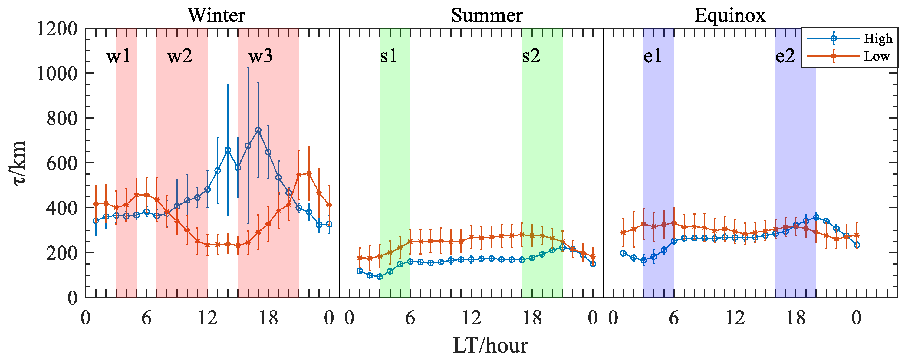
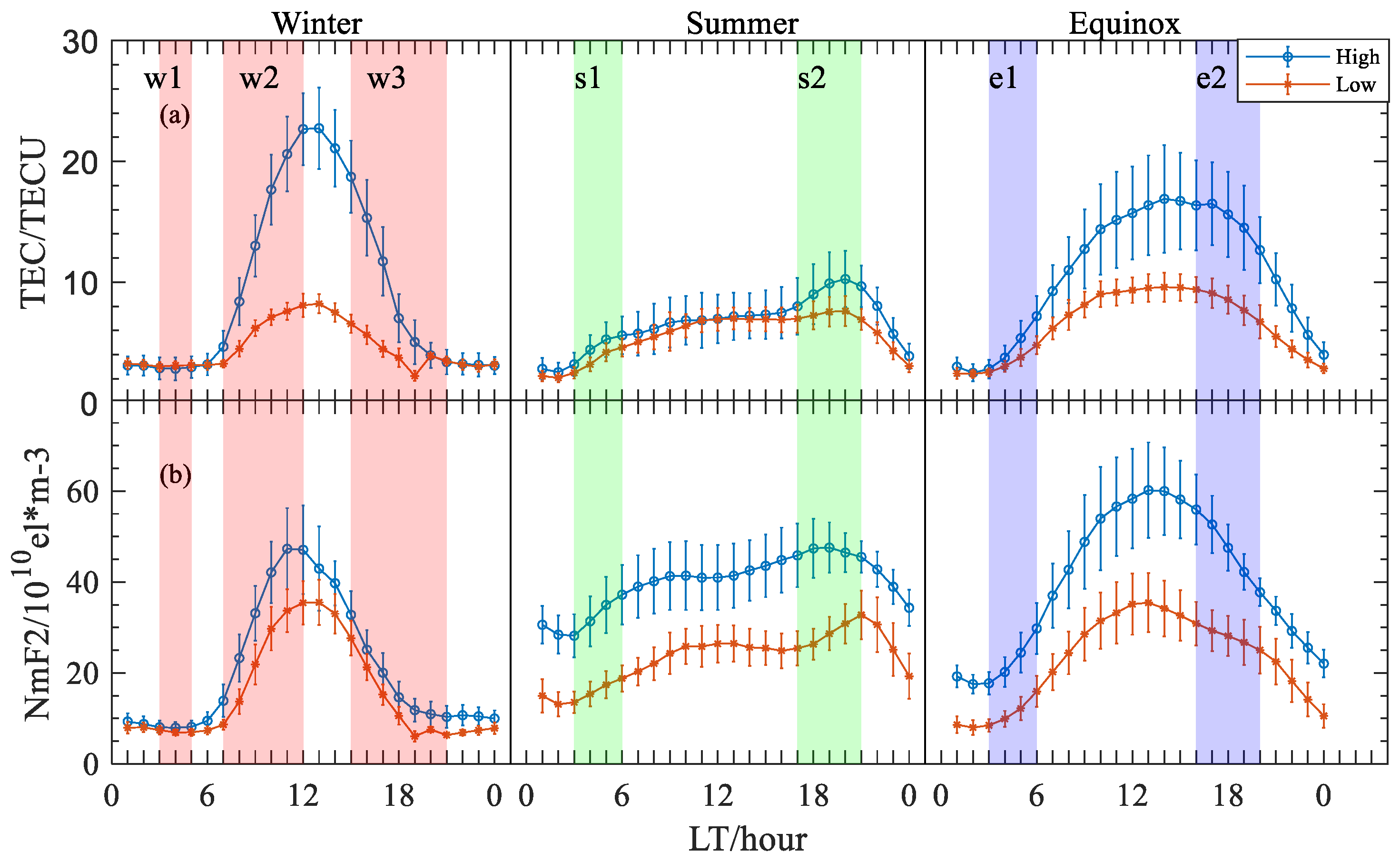
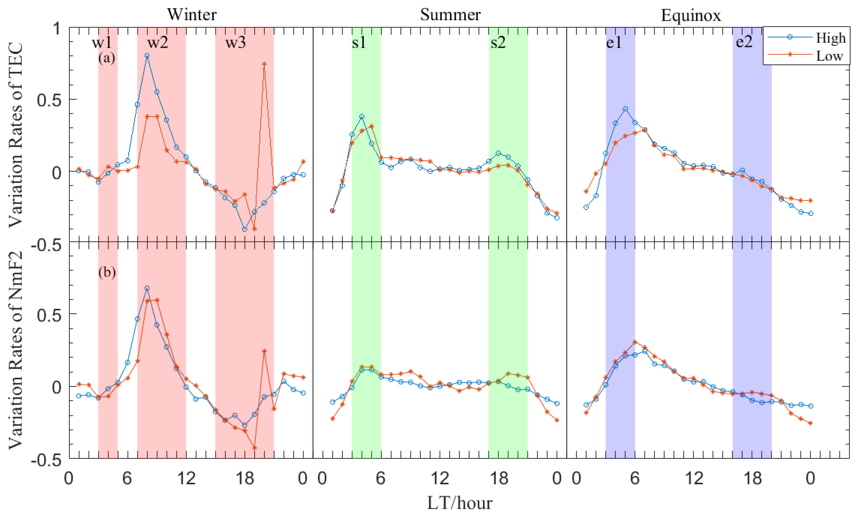
In winter, the τ in the high-solar-activity year shows an approximate single-peak pattern, while it displays a double-peak pattern in low-solar-activity years. Specifically speaking, the τ during the daytime is far larger than that in the nighttime in high-solar-activity years, whereas the opposite situation applies for low-solar-activity years. In the winter of the high-solar-activity year, the τ increases continuously after sunrise, reaching its first peak of 675 km at 14 LT, and then it decreases to 579 km at 15 LT and keeps increasing to the maximum of 746 km at 17 LT. After that, the τ decreases to its minimum 325 km at midnight 0 LT. In addition, it changed little during the midnight-to-sunrise period. On the other hand, the τ in the winter of low-solar-activity years showed a totally different pattern. It decreases to the minimum of 242 km in 12 LT during the pre-noon hours and continuously increases to the peak of 445 km at 22 LT. Moreover, it starts increasing at 3 LT and reaches its maximum of 480 km at 6 LT, as shown in Figure 3c.
(2)
In the summer, the τ has a similar variation both in the high- and low-solar-activity years, except that the τ has a post-sunset peak in high-solar-activity years, and τ in the high-solar-activity years is smaller than that in the low-solar-activity years during all periods, except in the evening period (20–22 LT). Specifically, in the high-solar-activity years, it stays relatively steady after sunrise, remaining in the 160 ± 10 km range. From 17 LT, it keeps increasing until it reaches the maximum of 225 km at 21 LT, and then it decreases to the minimum of 93 km at 3 LT. After that, the τ continuous increases to the pre-sunrise peak of 160 km at 5 LT. In the low-solar-activity years, it changed little during the sunrise-to-sunset period, remaining in the 235 ± 15 km range. Moreover, it begins to decrease after sunset, until it reaches a minimum of 161 km in 0 LT, and then it increases until the peak of 240 km at 6 LT.
(3)
In equinox, the τ in low-solar-activity years has a small range of diurnal variation, while in high-solar-activity years shows, it more variability, with τ having a maximum/minimum during the post-sunset/pre-sunrise period. Specifically speaking, it increases rapidly from 3 LT to its first peak of 264 km at 6 LT in high-solar-activity years. It remains stable (264–268 km) during the post-sunrise to afternoon (6–14 LT) period, and then it increases to the maximum of 357 km at 19 LT. From the evening to the post-midnight period (19–2 LT), the slab thickness decreases continuously to its minimum of 166 km at 2 LT. Compared with the τ in high-solar-activity years, the τ in low-solar-activity years shows less variability, especially during the pre-sunrise and post-sunset period, for which the τ does not have an apparent peak.
Figure 4. The diurnal variation of the mean and standard deviation of τ in different seasons of high and low-solar-activity years.
Remotesensing 14 05309 g004
This paper uses the DI index to evaluate the geomagnetic activity effect on the slab thickness, as described above. To demonstrate the difference of τ between storm time and quiet time, we first calculated the DI index during quiet time. According to whether the DI is positive or negative, the daily variation of the mean and standard deviation of the DI index are shown separately. The positive DI variation is represented by blue curves, and the negative DI variation is represented by red curves. As shown in Figure 5a, the magnitude of the ionospheric slab thickness perturbation at Yakutsk station is relatively stable at all times of the day, with the DI index fluctuating between −0.18 and 0.29. In addition, the disturbance is more intense during the sunset time compared with other periods, and the positive/negative DI index is at least greater than 0.21/less than −0.15 within 16:00–20:00 LT, with the DI index reaching a maximum/minimum of 0.29/−0.18, respectively, at 17:30 LT.
Figure 5b shows the variation of DI index during storm time. The variation of the storm-time DI index differs significantly from the variation of quiet-time DI index. The positive DI index in the storm time is far larger than that in the quiet time, with the smallest DI index at 0.32, which is greater than the largest positive DI index at 0.28 in quiet time. In the period from sunset to evening (17:00–23:00 LT), the storm-time positive DI index is less than 0.5. The DI index reached a peak of 1.14 at 2:30 LT after midnight, and another peak of 1.16 is also present at 12:00 LT. Overall, the most intense disturbances in τ and the corresponding largest DI indices were observed before midnight and around the midday hours. In contrast, during the sunset hours, when the DI index is the largest and the disturbance is the most intense on quiet days, the storm time disturbance is the weakest, and the DI index is the smallest. The negative DI index in storm time also shows a different morphology from that in the quiet time. It is relatively stable in the 11–17 LT period, with a value greater than −0.16. The negative perturbation is intense in the period after sunset to before midnight, with the minimum value of −0.29 at 21:00 LT. The negative DI index also reaches −0.27 at 1:00 LT after midnight and −0.25 at 8:00 LT after sunrise. Overall, the intensity of the positive and negative disturbance varies dramatically. The magnitude of the positive disturbance is much larger than the magnitude of the negative disturbance, and the local time variation of the positive/negative disturbance is also different.
To better show the geomagnetic effect on τ, Figure 6a presents the comparison of the quiet-time DI index and storm-time DI index. It is of great importance to note that the DI index in Figure 6a is the same as the mean DI index in Figure 5. As can be seen from the figure, the storm-time DI index has a greater range of variation than the quiet-time DI index. The storm-time positive DI index is larger than the quiet-time positive DI index in all periods, and it is particularly significant in the period from midnight to sunrise and around noon. The storm-time negative DI index has a more variable pattern compared to the quiet-time negative DI index. For most of the time, the storm-time negative DI index is smaller than the quiet-time negative DI index, except for the afternoon period from 12:00 to 15:00 LT when the storm-time negative DI index is slightly larger than the quiet-time negative DI index. Figure 6b shows the difference between the storm-time DI index and quiet-time DI index according to the sign of the DI index. As can be seen from the figure, the difference in the positive DI index is relatively small during the pre-sunset-to-evening period (17–23 LT), with the difference below 0.21. The difference is greater than 0.2 in all other time periods, reaching 0.93/1.02 at 02:45 LT/12:30 LT after midnight/around noon, respectively. On the other hand, the negative DI index difference is greater than -0.2 in all time periods, and even greater than 0 in the afternoon period, 12:00–15:00 LT, indicating that the negative disturbance during the storm is very weak. Therefore, we preliminarily conclude that the geomagnetic storm would enhance the τ at Yakutsk, especially for the τ in post-midnight-to-sunrise hours and noontime.

4. Discussion

Yakutsk is located at a high latitude in East Asia; the most important factors affecting the ionospheric climatological behavior in this region are solar radiation, solar zenith angle, and background atmospheric composition, which are associated with summer-to-winter prevailing circulation [46,47,48]. At the same time, the nighttime downward plasma influx from the plasmasphere and conjugate hemisphere can also significantly influence the ionospheric condition at high latitudes [49,50,51]. In addition, the geomagnetic activity could result in positive or negative ionospheric storms, which severely affect the ionosphere states, according to the local time, season, and other ionosphere–thermosphere system background information when the geomagnetic storms occur [52,53,54]. Consequently, the τ at Yakutsk shows a complicated pattern. Since the geomagnetic activity is the main contributor to the relative ionospheric variability, we first discussed the climatology of τ, followed by the variation of τ in storm time.
To explain the diurnal variation of τ, the TEC and NmF2 during the same geomagnetic quiet period as the period of τ shown in Figure 4 are selected, and we displayed them in Figure 7, according to the definition of τ. It can be seen from the figure that TEC and NmF2 have different morphology in different seasons at high latitudes. The reversal of the meridional wind to equatorward and continuous strong solar radiation in the summer leads to a pronounced increase in TEC and NmF2 during post-sunset period [51,55,56,57]. Moreover, the TEC and NmF2 in Yakutsk display different magnitude ‘winter anomaly’ which referred to the TEC and NmF2 around noontime in winter being larger than those in summer [47,58]. Specifically, the “winter anomaly” of TEC is more evident in the high-solar-activity year, while the “winter anomaly” of NmF2 is more significant in the low solar activity years, consistent with previous studies [48]. It is due to the ionosphere strongly depending on the solar zenith angle in the winter, and the increasing [O/N2] is less/more important than the strong/weak solar radiation in high- and low-solar-activity years, respectively. Therefore, the TEC around noontime is greatest in winter of high-solar-activity years, and it caused the maximum of τ, while the large NmF2 caused the small τ in winter of low-solar-activity years, as shown in Figure 7. Moreover, the Yakutsk Anomaly (YA) is similar to the Weddell Sea Anomaly (WSA), which is characterized by greater nighttime electron density than daytime electron density in summer, as also seen in Figure 6, consistent with previous sub-auroral summer longitudinal anomalies study [59,60,61].
Moreover, we could also calculate the variation rates of τ, which are determined by the variation rates of TEC and NmF2 as follows (deduced from Equation (1)):
d τ d t = 1 N m F 2 d T E C d t     T E C N m F 2 2 d N m F 2 d t
Figure 8 presents the temporal variation rates of TEC and NmF2. According to Equation (3): The increase in variation rates of τ can be classified into the following groups (1) TEC increases and NmF2 drops; (2) TEC and NmF2 rise, but the variation rates of TEC are larger than that of NmF2; and (3) TEC and NmF2 fall, but the variation rates of NmF2 is smaller than that of TEC. The opposite situation applies to the decrease in τ.
As the τ has a totally different diurnal variation in the winter of the high- and low-solar-activity year, we discussed the physical mechanism related to the phenomenon first. As the Yakutsk is located at a high latitude, the solar zenith angle is small and the duration of solar radiation is short in the winter. Therefore, the electron density is highly sensitive to the solar zenith angle in this region [48]. In the high-solar-activity year, the variation rates of TEC are larger than that of NmF2 due to the solar zenith angle increases, although the summer-to-winter circulation would attenuate it (the increase of NmF2 caused by circulation is greater than that of TEC as the main area affected by summer to winter circulation is near the peak height of F2 layer) [47,62]. In other words, the solar zenith angle is more important than the prevailing wind circulation to TEC and NmF2 in high latitudes. Therefore, in the w2 period of the high-solar-activity year, the variation rate of TEC is greater than that of NmF2, and τ is increased. On the other hand, the variation rates of TEC and NmF2 are small in the w2 period of low-solar-activity years due to the low solar radiation in the low-solar-activity year. At the same time, the prevailing summer-to-winter circulation also influences the ionosphere significantly. As the summer-to-winter circulation mainly affects the area near the peak height of the F2 layer, it would result in the NmF2 increase faster than TEC, as shown in Figure 7. Therefore, the τ decreases during the w2 period in the low solar activity. In addition, the opposite situations could explain the increases of τ in low-solar-activity years. As the prevailing circulation effect attenuate, it would result in the decrease in rates of TEC smaller than that of NmF2, and the τ would therefore increase in the first half of the W3 period.
Around sunset hours, the decrease of the O+-H+ conversion height (i.e., the increase of the downward influx of the plasmasphere) also led to the increase of the τ in the winter of the low solar activity year (second half of the W3 period). The weak solar radiation around sunset in winter will not cause an obvious TEC increase, and the increase of TEC and NmF2 after sunset in low solar activity years shown in the figure is due to the lower O+-H+ conversion height. Previous studies also suggested that the decrease of the O+-H+ conversion height has a negative correlation with solar activity, as with the lower recombination rates in low-solar-activity years [63]. As the recombination rates are lower in high altitudes, in the process of downward influx from the plasmasphere and conjugate hemisphere, the increase of TEC is more than that of NmF2, resulting in the increase of τ around sunset in winter of low-solar-activity years. It can also be seen from Figure 4 that there is an increase of τ in the w1 period in low-solar-activity years, and it should also be attributed to the plasma transport from the plasmasphere and conjugate hemisphere. As the w1 period is 2–4 LT before sunrise in winter, the meridional wind is still equator-ward during the period, and the plasmasphere is not exposed to solar radiation. Therefore, NmF2 does not decrease rapidly, and TEC does not increase significantly, as shown in Figure 7, and the peak of the W1 time period is due to the decrease of the O+-H+ transition height, i.e., the transport of plasma flux. As the transport process is downward, and the ionosphere at higher heights than hmF2 has a recombination rate, the variation rates of TEC are, therefore, larger than those of NmF2, resulting in the increases of τ in the w1 period.
As for the τ variation in the summer and equinox, it can be seen from Figure 7 that TEC and NmF2 increase in the summer s1 period, as well as in the equinox e1 period, while it is not a nighttime increase. Because the increases in TEC and NmF2 are due to the change of solar zenith angel during this period at high latitudes, as indicated by Figure 7 the TEC and NmF2 increase continuously even after the s1 and e1 periods, and the increases in τ during the s1 and e1 periods are caused by the greater effect of the solar zenith angle on TEC than on NmF2 after sunrise.
Figure 7 also shows that TEC, as well as NmF2 is still increasing after 18 LT in summer (s2 period), which is due to the change of wind direction from poleward to equatorward around dusk hours and the continuous solar radiation after sunset [64,65]. On the one hand, the equatorward wind would raise the ionosphere to higher altitudes, where the recombination rates of electrons are lower. On the other hand, the topside ionosphere (along with the plasmasphere) is exposed to solar radiation for a longer time than the bottomside ionosphere, and the solar radiation is strong in the high-solar-activity year, so the increase rate of TEC is larger than that of NmF2, causing the τ increases in the s2 time period in high-solar-activity year. Due to the lack of sufficient solar radiation intensity in the equinox, the equatorward wind at sunset could not cause an increase in TEC and NmF2; however, they would cause the rate of decrease in TEC to be less than the rate of decrease in NmF2, which in turn leads to an increase in τ during e2 period. Additionally, as the wind reversal mainly influences the height around hmF2 and the solar irradiance is low in the low-solar-activity years, the increase/decrease rate of NmF2 is more intense/weak than the increase/decrease rate of TEC during the dusk period in the summer low-solar-activity years, resulting the decrease of τ in s2/e2 period in low-solar-activity years.
The geomagnetic storm is an important factor affecting the ionosphere, as it can severely disturb the ionosphere–thermosphere system through various process. Previous studies have found that the correlation between the τ and geomagnetic activity seems to be different for varying location, local time, season, solar activity, and magnetic activity intensity [27,33,34]. As for the effect of geomagnetic storms on the τ in high latitudes, Jayachandran et al. [36] found that the τ would increase throughout the day at Goose Bay, which is located in high latitudes during both the solar minimum year (1985) and solar maximum (1981) by comparing the τ in geomagnetically quiet days (Ap < 10) and geomagnetically disturbed days. In this paper, we also found that the storm-time positive DI index is larger than the quiet-time positive DI index throughout the day, suggesting that the τ tends to increase during geomagnetic storms. By contrast, the negative DI index of τ during storm time varies little from that of the quiet-time negative DI index, which is larger than −0.2 during both daytime and nighttime, indicating that the negative disturbance of τ during magnetic storms is weak.
During geomagnetic storms, there are several processes affecting the τ, and these processes include the following: (1) prompt penetration of the electric field due to the imbalance between the R1 (region1) and R2 (region 2) field-aligned currents FAC; (2) disturbance dynamo electric field due to the storm-time equatorward winds; (3) equatorward neutral wind result from the particle precipitation and Joule heating at high latitude, sometimes accompanied with traveling atmosphere disturbance (TAD); and (4) composition changes caused by the expansion of the neutral atmosphere at high latitudes and transport by the equatorward winds. In addition, there are two important processes that could affect the ionosphere at high latitudes during geomagnetic storms [55]. The particle precipitation gets stronger as there are more energetic particles input to the ionosphere through the nearly perpendicular field line during storms. At the same time, the cross-polar-cap potential drop increases significantly, resulting in the intensification and expansion of the plasma convection pattern. In the following, we present an example on 7 June 2013 to analyze why the τ would increase during the geomagnetic storms. Note that the Dst variation during the geomagnetic storm was presented in Figure 2.
Figure 9 shows the variations of the DI index of TEC, NmF2, and τ during the period from 6 June 12 UT to 8 June 0 UT. Correspondingly, the TEC/NmF2 observations and their monthly median were also presented in Figure 9. It can be seen from the figure that there is an interrupted TEC increase in 0 UT on 7 June, resulting in a TEC positive disturbance that lasts for 12 h (S1 period). Meanwhile, the NmF2 observations are smaller than the corresponding monthly median, and there are negative disturbances of NmF2. Therefore, the τ increases markedly, and there are positive disturbances of τ during the s1 period.
It is generally accepted that the PPEF, DDEF, equatorward neutral wind, and composition changes could influence the ionosphere of different altitudes in a similar way [40,55]. In addition, the ionospheric background and dominant physical process are different for varying altitudes. Therefore, the responses of TEC and NmF2 to geomagnetic storms often behave in a similar way but with different magnitudes for geomagnetic storm periods. Figure 9 shows that there is a contrasting behavior between the TEC and NmF2 during the s1 period, resulting in the positive disturbance of τ. Hence, there might have been other processes affecting the ionosphere at Yakutsk during the storm time. The particle precipitation and convection electric field are two important processes influencing the high-latitude ionosphere. As previous studies suggested, the particle precipitation mainly occurred in the cusp and auroral E region, which are a source of substantial ionization [66,67]. During geomagnetic storms, there is intense particle precipitation in the E region, and the high-energy precipitating particles collide with the neutral composition, resulting the high electron density in the E region. Meanwhile, the plasma convection intensifies and expands to lower latitudes during the storm. Therefore, the increased electron density in the E region could circulate to Yakutsk station through the storm-time, thus expanding plasma convection electric field and resulting in the electron density enhancement in the E region at Yakutsk. On the other hand, the intensified convection electric field would cause the recombination rate of the electron density in the F region to become stronger and electron density decreases. Consequently, the electron density in the E region could be larger than that in the F region. Previous studies have also found that the total electron content in the E region (TEC_E) could be a major component of the total electron content (TEC) during the geomagnetic storms [68,69]. Therefore, we preliminarily infer that it is the intense particle precipitation and expanding magnetospheric convection electric field during the storm that causes the TEC to increase even as NmF2 decreases during the s1 period. More observations and modeling work will be conducted in the future to study the physical mechanism of the storm-time τ increases at Yakutsk.

5. Conclusions

This paper presents a statistical analysis of the ionospheric slab thickness τ at Yakutsk which is located in the high latitude of East Asia, using the TEC and NmF2 data during the years 2010–2017. The results show that τ has great local time, seasonal and solar activity variation, and the climatology of the τ is distinct from that in other high latitude regions. In addition, the geomagnetic storm seems to have a positive effect on the τ, consistent with previous study [36]. The main conclusions of this study are summarized as follows:
(1)
The τ is greatest in the winter, followed by the equinox; and it is smallest in summer in both high- and low-solar-activity years, except in the noontime of low-solar-activity years. It is due to the ionosphere strongly depending on the solar zenith angle in the winter at Yakutsk, and the increasing [O/N2] is less/more important than the strong/weak solar radiation in high- and low-solar-activity years, respectively.
(2)
In the winter, the τ in high-solar-activity years shows an approximate single-peak pattern around noontime, while it displays a double peak in pre-sunrise and post-sunset periods in low-solar-activity years. In the high-solar-activity years, the noon-time peak was caused by the fact that the solar zenith angle is more important than the prevailing wind circulation to t TEC and NmF2 in Yakutsk. In the low solar activity years, the post-sunset and pre-sunrise peaks were caused by the downward plasma influx from the plasmasphere and conjugate hemisphere.
(3)
In the summer and equinox, there is an increase during the forenoon period due to the greater effect of the solar zenith angle on TEC than on NmF2 in the period. In addition, there are post-sunset peaks in summer and equinox of high-solar-activity years, and they were caused by the equatorward neutral wind and continuous strong solar radiation in summer and equinox.
(4)
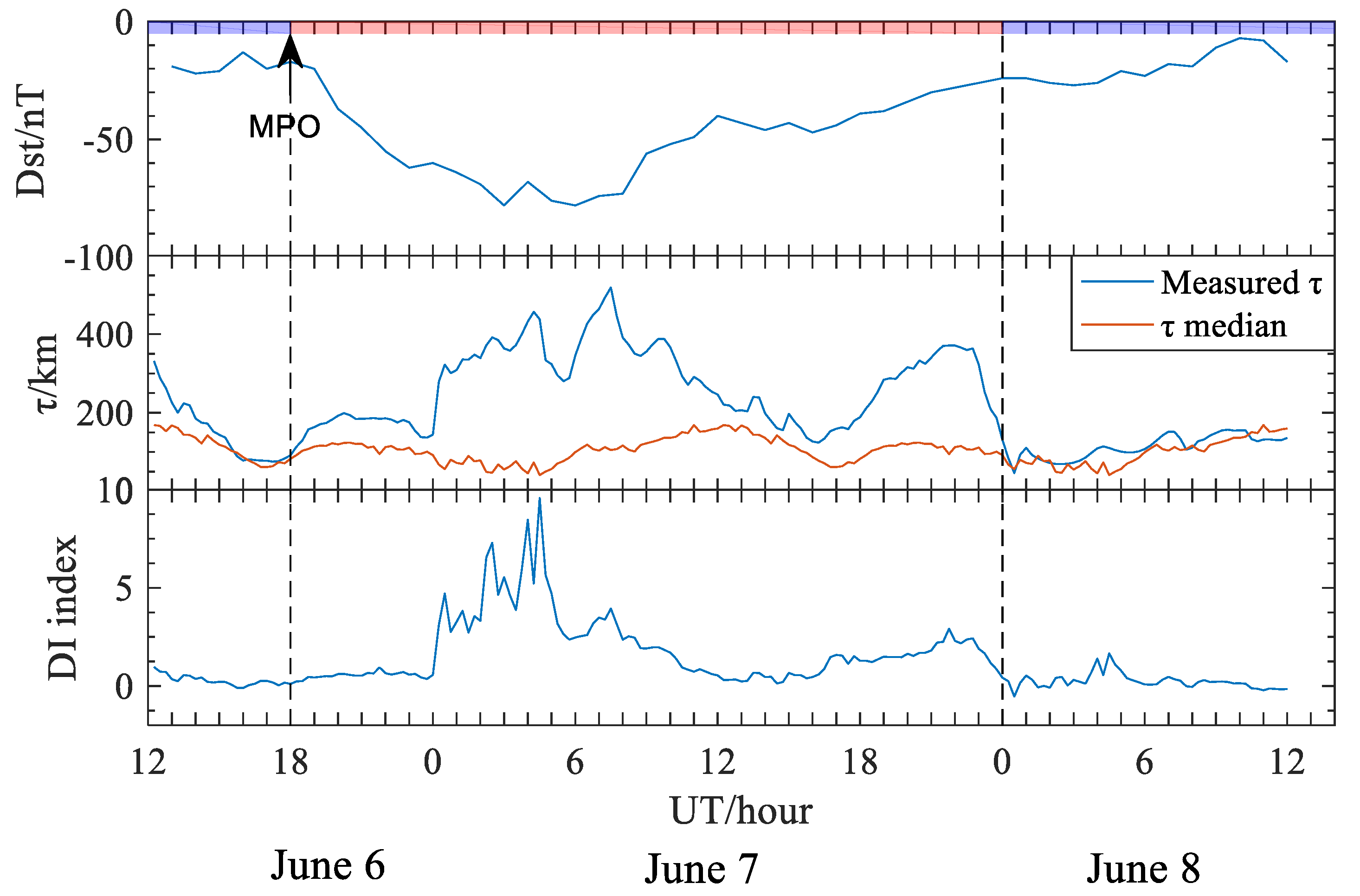
Geomagnetic storms seem would enhance τ during the storm period, and this effect should be associated with intense particle precipitation and expanded plasma convection electric field during the storm time.

Author Contributions

Conceptualization, Y.Z. (Yuqiang Zhang), J.F. and N.X.; methodology, Z.D.; investigation, Y.L. and C.Z.; validation, J.F. and B.C.; formal analysis, Y.Z. (Yuqiang Zhang) and Z.W. (Zhuangkai Wang); resources, Y.Z. (Yufeng Zhou) and Z.Z.; visualization, J.F. and Z.W. (Zhensen Wu); funding acquisition, Y.L. and T.X. All authors have read and agreed to the published version of the manuscript.

Funding

This work was supported by the foundation of National Key Laboratory of Electromagnetic Environment (Grant No. 20200101), the Fundamental Research Funds for the Central Universities (Grant No. 2042021kf0022), the Stable-Support Scientific Project of China Research Institute of Radiowave Propagation (Grant No. A132102W06), the National Natural Science Foundation of China (Grant Nos. 42074187 and 42204161), the National Key R&D Program of China (Grant No. 2018YFC1503506), the Excellent Youth Foundation of Hubei Provincial Natural Science Foundation (Grant No. 2019CFA054), and Stable Support Project of Basic Scientific Research Institutes (Grant No. A131901W10).

Data Availability Statement

The use of ionosonde data provided by GIRO (Global Ionospheric Radio Observation) database (https://giro.uml.edu/didbase, (accessed on 20 October 2022)). The use of GPS data provided by UNAVCO database (University NAVSTAR Consortium) (http://www.unavco.org/, (accessed on 20 October 2022)). The use of Dst data provided by WDC (World Data Center, http://wdc.kugi.kyoto-u.ac.jp/, (accessed on 20 October 2022)). The use of F10.7 data provided by NOAA (ftp://ftp.swpc.noaa.gov/pub/indices/old_indices/, (accessed on 20 October 2022)).

Acknowledgments

We acknowledge the use of ionosonde data provided by GIRO (Global Ionospheric Radio Observation) database (https://giro.uml.edu/didbase, (accessed on 20 October 2022)), GPS data provided by UNAVCO database (University NAVSTAR Consortium) (http://www.unavco.org/, (accessed on 20 October 2022)), Dst data provided by WDC (http://wdc.kugi.kyoto-u.ac.jp/, (accessed on 20 October 2022)), and F10.7 data provided by NOAA (ftp://ftp.swpc.noaa.gov/pub/indices/old_indices/, (accessed on 20 October 2022)).

Conflicts of Interest

The authors declare no conflict of interest.

References

  1. Wright, J.W. A model of the F-region above hmaxF2. J. Geophys. Res. 1960, 65, 185–191. [Google Scholar] [CrossRef]
  2. Rishbeth, H.; Garriott, O. Introduction to Ionospheric Physics; International Geophysics Series; Academic Press: New York, NY, USA, 1969; Volume 14. [Google Scholar]
  3. Titheridge, J.E. The ionospheric slab thickness of the mid-latitude ionosphere. Planet Space Sci. 1973, 21, 1775–1793. [Google Scholar] [CrossRef]
  4. Jakowski, N.; Putz, E.; Spalla, P. Ionospheric storm characteristics deduced from satellite radio beacon observations at three European stations. Ann. Geophys. 1990, 8, 343–352. [Google Scholar]
  5. Jakowski, N.; Mielich, J.; Hoque, M.M.; Danielides, M. Equivalent ionospheric slab thickness at the mid-latitude ionosphere during solar cycle 23. In Proceedings of the 38th COSPAR Scientific Assembly, Bremen, Germany, 18–25 July 2010. [Google Scholar]
  6. Jakowski, N.; Hoque, M.M. Global equivalent ionospheric slab thickness model of the Earth’s ionosphere. J. Space Weather Space Clim. 2021, 11, 10. [Google Scholar] [CrossRef]
  7. Pignalberi, A.; Pezzopane, M.; Rizzi, R. Modeling the lower part of the topside ionospheric vertical electron density profile over the European region by means of Swarm satellites data and IRI UP method. Space Weather 2018, 16, 304–320. [Google Scholar] [CrossRef]
  8. Pignalberi, A.; Pezzopane, M.; Themens, D.R.; Haralambous, H.; Nava, B.; Coïsson, P. On the analytical description of the topside ionosphere by NeQuick: Modeling the scale height through COSMIC/FORMOSAT-3 selected data. IEEE J. Sel. Top. Appl. Earth Obs. Remote Sens. 2020, 13, 1867–1878. [Google Scholar] [CrossRef]
  9. Mendillo, M.; Papagiannis, M.D.; Klobuchar, J.A. Average behavior of the midlatitude F-region parameters NT, Nmax and τ during geomagnetic storms. J. Geophys. Res. 1972, 77, 4891–4895. [Google Scholar] [CrossRef]
  10. Krankowski, A.; Shagimuratov, I.I.; Baran, L.W. Mapping of foF2 over Europe based on GPS-derived TEC data. Adv. Space Res. 2007, 39, 651–660. [Google Scholar] [CrossRef]
  11. Gerzen, T.; Jakowski, N.; Wilken, V.; Hoque, M.M. Reconstruction of F2 layer peak electron density based on operational vertical total electron content maps. Ann. Geophys. 2013, 31, 1241–1249. [Google Scholar] [CrossRef] [Green Version]
  12. Maltseva, O.A.; Mozhaeva, N.S.; Nikitenko, T.V. Validation of the Neustrelitz Global Model according to the low latitude ionosphere. Adv. Space Res. 2014, 54, 463–472. [Google Scholar] [CrossRef]
  13. Frόn, A.; Galkin, I.; Krankowski, A.; Bilitza, D.; Hernández-Pajares, M.; Reinisch, B.; Li, Z.; Kotulak, K.; Zakharenkova, I.; Cherniak, I.; et al. Towards Cooperative Global Mapping of the Ionosphere: Fusion Feasibility for IGS and IRI with Global Climate VTEC Maps. Remote Sens. 2020, 12, 3531. [Google Scholar] [CrossRef]
  14. Galkin, I.; Frόn, A.; Reinisch, B.; Hernández-Pajares, M.; Krankowski, A.; Nava, B.; Bilitza, D.; Kotulak, K.; Flisek, P.; Li, Z.; et al. Global monitoring of ionospheric weather by GIRO and GNSS data fusion. Atmosphere 2022, 13, 371. [Google Scholar] [CrossRef]
  15. Bhonsle, R.V.; Da Rosa, A.V.; Garriott, O.K. Measurement of Total Electron Content and the Equivalent ionospheric slab thickness of the Mid latitude Ionosphere. Radio Sci. 1965, 69, 929–937. [Google Scholar]
  16. Huang, Y.N. Some results of ionospheric slab thickness observations at Lunping. J. Geophys. Res. 1983, 88, 5517–5522. [Google Scholar] [CrossRef]
  17. Davies, K.; Liu, X.M. Ionospheric slab thickness in middle and low latitudes. Radio Sci. 1991, 26, 997–1005. [Google Scholar] [CrossRef]
  18. Fox, M.W.; Mendillo, M.; Klobuchar, J.A. Ionospheric equivalent ionospheric slab thickness and its modeling applications. Radio Sci. 1991, 26, 429–438. [Google Scholar] [CrossRef]
  19. Chuo, Y.J.; Lee, C.C.; Chen, W.S. Comparison of ionospheric equivalent slab thickness with bottomside digisonde profile over Wuhan. J. Atmos. Sol.-Terr. Phys. 2010, 72, 528–533. [Google Scholar] [CrossRef]
  20. Jin, S.; Cho, J.-H.; Park, J.-U. Ionospheric slab thickness and its seasonal variations observed by GPS. J. Atmos. Sol. Terr. Phys. 2007, 69, 1864–1870. [Google Scholar] [CrossRef]
  21. Stankov, S.M.; Warnant, R. Ionospheric slab thickness—Analysis, modelling and monitoring. Adv. Space Res. 2009, 44, 1295–1303. [Google Scholar] [CrossRef]
  22. Guo, P.; Xu, X.; Zhang, G.X. Analysis of the ionospheric equivalent ionospheric slab thickness based on ground-based GPS/TEC and GPS/COSMIC RO. J. Atmos. Sol. Terr. Phys. 2011, 73, 839–846. [Google Scholar] [CrossRef]
  23. Huang, H.; Liu, L.; Chen, Y.; Le, H.; Wan, W. A global picture of ionospheric slab thickness derived from GIM TEC and COSMIC radio occultation observations. J. Geophys. Res. Space Phys. 2016, 121, 867–880. [Google Scholar] [CrossRef]
  24. Odeyemi, O.O.; Adeniyi, J.O.; Oladipo, O.A.; Olawepo, A.O.; Adimu, I.A.; Oyeyemi, E.O. Ionospheric slab thickness investigation on slab-thickness and B0 over an equatorial station in Africa and comparison with IRI model. J. Atmos. Sol. Terr. Phys. 2018, 179, 293–306. [Google Scholar] [CrossRef]
  25. Jakowski, N.; Hoque, M.M.; Mielich, J.; Hall, C. Equivalent ionospheric slab thickness of the ionosphere over Europe as an indicator of long-term temperature changes in the thermosphere. J. Atmos. Terr. Phys. 2017, 163, 92–101. [Google Scholar]
  26. Pignalberi, A.; Nava, B.; Pietrella, M.; Cesaroni, C.; Pezzopane, M. Mid-latitude climatology of the ionospheric equivalent slab thickness over two solar cycles. J. Geod. 2021, 95, 124. [Google Scholar] [CrossRef]
  27. Kersley, L.; Hajeb-Hosseinieh, H. Dependence of ionospheric slab thickness on geomagnetic activity. J. Atmos. Terr. Phys. 1976, 38, 1357–1360. [Google Scholar] [CrossRef]
  28. Venkatesh, K.; Rama Rao, P.V.S.; Prasad, D.S.V.V.D.; Niranjan, K.; Saranya, P.L. Study of TEC, slab thickness and neutral temperature of the thermosphere in the Indian low latitude sector. Ann. Geophys. 2011, 29, 1635–1645. [Google Scholar] [CrossRef] [Green Version]
  29. Minakoshi, H.; Nishimuta, I. Ionospheric electron content and equivalent ionospheric slab thickness at lower mid-latitudes in the Japanese zon. In Proceedings of the Beacon Satellite Symposium (IBSS), Aberystwyth, UK, 11–15 July 1994; University of Wales: Wales, UK, 1994; Volume 144. [Google Scholar]
  30. Gulyaeva, T.L.; Jayachandran, B.; Krishnankutty, T.N. Latitudinal variation of slab thickness. Adv. Space Res. 2004, 33, 862–865. [Google Scholar] [CrossRef]
  31. Huang, Z.; Yuan, H. Climatology of the ionospheric slab thickness along the longitude of 120°E in China and its adjacent region during the solar minimum years of 2007–2009. Ann. Geophys. 2015, 33, 1311–1319. [Google Scholar] [CrossRef] [Green Version]
  32. Balan, N.; Iyer, N. Ionospheric slab thickness during geomagnetic storm. Indian J. Radio Space Phys. 1978, 7, 238–241. [Google Scholar]
  33. Breed, A.M.; Goodwin, G.L.; Vandenberg, A.-M.; Essex, E.A.; Lynn, K.J.W.; Silby, J.H. Ionospheric total electron content and ionospheric slab thickness determined in Australia. Radio Sci. 1997, 62, 1635–1643. [Google Scholar] [CrossRef]
  34. Pignalberi, A.; Pietrella, M.; Pezzopane, M.; Nava, B.; Cesaroni, C. The Ionospheric Equivalent Slab Thickness: A Review Supported by a Global Climatological Study Over Two Solar Cycles. Space Sci. Rev. 2022, 218, 37. [Google Scholar] [CrossRef]
  35. Zhang, Y.; Wu, Z.; Feng, J.; Xu, T.; Deng, Z.; Ou, M.; Xiong, W.; Zhen, W. Statistical study of ionospheric equivalent slab thickness at Guam magnetic equatorial location. Remote Sens. 2021, 13, 5175. [Google Scholar] [CrossRef]
  36. Jayachandran, B.; Krishnankutty, T.; Gulyaeva, T. Climatology of ionospheric slab thickness. Ann. Geophys. 2004, 22, 25–33. [Google Scholar] [CrossRef] [Green Version]
  37. Yadav, R.; Bhawre, P. Ionospheric slab thickness over high latitude Antarctica during the maxima of solar cycle 23rd. Int. J. Curr. Res. 2020, 12, 10041–10046. [Google Scholar] [CrossRef]
  38. Abe, O.; Villamide, X.O.; Paparini, C.; Radicella, S.; Nava, B.; Rodríguez Bouza, M. Performance evaluation of GNSS-tec ionospheric slab thickness estimation techniques at the grid point in middle and low latitudes during different geomagnetic conditions. J. Geod. 2017, 91, 409–417. [Google Scholar] [CrossRef]
  39. Uwamahoro, J.C.; Giday, N.M.; Habarulema, J.B.; Katamzi-Joseph, Z.T.; Seemala, G.K. Reconstruction of storm-time total electron content using ionospheric tomography and artificial neural networks: A comparative study over the African region. Radio Sci. 2018, 53, 1328–1345. [Google Scholar] [CrossRef]
  40. Seemala, G.; Valladares, C. Statistics of total electron content depletions observed over the South American continent for the year 2008. Radio Sci. 2011, 46, RS5019. [Google Scholar] [CrossRef]
  41. Olwendo, O.; Baki, P.; Mito, C.; Doherty, P. Characterization of ionospheric GPS Total Electron content (GPS TEC) in low latitude zone over the Kenyan region during a very low solar activity phase. J. Atmos. Sol. Terr. Phys. 2012, 84, 52–61. [Google Scholar] [CrossRef]
  42. Matamba, T.M.; Habarulema, J.B.; McKinnell, L.-A. Statistical analysis of the ionospheric response during geomagnetic storm conditions over South Africa using ionosonde and GPS data. Space Weather 2015, 13, 536–547. [Google Scholar] [CrossRef]
  43. De Dieu Nibigira, J.; Sivavaraprasad, G.; Ratnam, D.V. Performance analysis of IRI-2016 model TEC predictions over Northern and Southern Hemispheric IGS stations during descending phase of solar cycle 24. Acta Geophys. 2021, 69, 1509–1527. [Google Scholar] [CrossRef]
  44. Reinisch, B.W.; Galkin, T.A. Global ionospheric radio observatory (GIRO). Earth Planets Space 2011, 63, 377–381. [Google Scholar] [CrossRef] [Green Version]
  45. Gulyaeva, T.; Stanislawska, I. Night-day imprints of ionospheric slab thickness during geomagnetic storm. J. Atmos. Sol. Terr. Phys. 2005, 67, 1307–1314. [Google Scholar] [CrossRef]
  46. Fuller Rowell, T.J.; Rees, D. Derivation of a conservation equation for mean molecular weight for a two constituent gas within a three dimensional time-dependent model of the thermosphere. Planet. Space Sci. 1983, 31, 1209–1222. [Google Scholar] [CrossRef]
  47. Rishbeth, H. How the thermospheric circulation affects the ionosphere F2-layer. J. Atmos. Terr. Phys. 1998, 60, 1385–1402. [Google Scholar] [CrossRef]
  48. Ma, R.; Xu, J.; Wang, W.; Yuan, W. Seasonal and latitudinal differences of the saturation effect between ionospheric NmF2and solar activity indices. J. Geophys. Res. 2009, 114, A10303. [Google Scholar]
  49. Bailey, G.J.; Sellek, R.; Balan, N. The effect of interhemispheric coupling on nighttime enhancements in ionospheric total electron content during winter at solar minimum. Ann. Geophys. 1991, 9, 738–747. [Google Scholar]
  50. Jakowski, N.; Förster, M. About the nature of the Night-time Winter Anomaly effect (NWA) in the F-region of the ionosphere. Planet. Space Sci. 1995, 43, 603–612. [Google Scholar] [CrossRef]
  51. Chen, Y.; Liu, L.; Le, H.; Wan, W.; Zhang, H. The global distribution of the dusk-to-nighttime enhancement of summer NmF2 at solar minimum. J. Geophys. Res. Space Res. 2016, 121, 7914–7922. [Google Scholar] [CrossRef]
  52. Fuller-Rowell, T.J.; Codrescu, M.V.; Moffett, R.J.; Quegan, S. Response of the thermosphere and ionosphere to geomagnetic storm. J. Geophys. Res. Atmos. 1994, 99, 3893–3914. [Google Scholar] [CrossRef]
  53. Buonsanto, M.J. Ionospheric storms—A review. Space Sci. Rev. 1999, 88, 563–601. [Google Scholar] [CrossRef]
  54. Mendillo, M. Storms in the ionosphere: Patterns and processes for total electron content. Rev. Geophys. 2006, 44, 335–360. [Google Scholar] [CrossRef]
  55. Bellchambers, W.; Piggott, W. Ionospheric measurements made at Halley Bay. Nature 1958, 182, 1596–1597. [Google Scholar] [CrossRef]
  56. Horvath, I.; Essex, E.A. The Weddell sea anomaly observed with the Topex satellite data. J. Atomos. Sol. Terr. Phys. 2003, 65, 693–706. [Google Scholar] [CrossRef]
  57. Lin, C.H.; Liu, J.Y.; Cheng, C.Z.; Chen, C.H.; Liu, C.H.; Wang, W.; Burns, A.G.; Lei, J. Three-dimensional ionospheric electron density structure of the Weddell Sea Anomaly. J. Geophys. Res. Space Res. 2009, 114, A02312. [Google Scholar] [CrossRef] [Green Version]
  58. Duncan, R.A. F-region seasonal and magnetic-storm behavior. J. Atmos. Terr. Phys. 1969, 31, 59–70. [Google Scholar] [CrossRef]
  59. Mamrukov, A.P. Evening anomalous enhancement of ionization in F region. Geomagn. Aeron. 1971, 21, 984–988. [Google Scholar]
  60. Maxim, K.; Vladimir, K.; Alexander, K.; Konstantin, R. Sub-auroral longitudinal anomalies in ionosphere-protonosphere system according to GSM TIP model and IK-19 satellite and ground-based observation. In Proceedings of the 2014 XXXIth URSI General Assembly and Scientific Symposium (URSI GASS), Beijing, China, 16–23 August 2014; pp. 1–4. [Google Scholar] [CrossRef]
  61. Richards, P.G.; Meier, R.R.; Chen, S.; Dandenault, P. Investigation of the Causes of the Longitudinal and Solar Cycle Variation of the Electron Density in the Bering Sea and Weddell Sea Anomalies. J. Geophys. Res. Space Res. 2018, 123, 7825–7842. [Google Scholar] [CrossRef]
  62. Torr, D.G.; Torr, M.R.; Richards, P.G. Causes of the F region winter anomaly. Geophys. Res. Lett. 1980, 7, 301–304. [Google Scholar] [CrossRef]
  63. Jakowski, N.; Hoque, M.M.; Kriegel, M.; Patidar, V. The persistence of the NWA effect during the low solar activity period 2007–2009. J. Geophys. Res. Space Phys. 2015, 120, 9148–9160. [Google Scholar] [CrossRef]
  64. He, M.; Liu, L.; Wan, W.; Ning, B.; Zhao, B.; Wen, J.; Yue, X.; Le, H. A study of the Weddell Sea Anomaly observed by FORMOSAT-3/COSMIC. J. Geophys. Res. Space Res. 2009, 114, A1230. [Google Scholar] [CrossRef] [Green Version]
  65. Xiong, C.; Lühr, H. The Midlatitude Summer Night Anomaly as observed by CHAMP and GRACE: Interpreted as tidal features. J. Geophys. Res. Space Res. 2014, 119, 4905–4915. [Google Scholar] [CrossRef] [Green Version]
  66. Roble, R.G. The Polar Lower Thermosphere. Planet. Space Sci. 1992, 40, 271–297. [Google Scholar] [CrossRef]
  67. Robel, R.G.; Rees, M.H. Time-dependent studies of the aurora: Effects of particle precipitation on the dynamic morphology of ionospheric and atmospheric properties. Planet. Space Sci. 1977, 25, 991–1010. [Google Scholar] [CrossRef]
  68. Wu, Y.; Liu, R.; Zhang, B.; Wu, Z.; Hu, H.; Zhang, S.; Zhang, Q.; Liu, J.; Honary, F. Multi-instrument observations of plasma features in the Arctic ionosphere during the main phase of a geomagnetic storm in December 2006. J. Atmos. Sol. Terr. Phys. 2013, 105–106, 358–366. [Google Scholar] [CrossRef]
  69. Yang, S.; Zhang, B.; Fang, H.; Liu, J.; Zhang, Q.; Hu, H.; Liu, R.; Li, C. F-lacuna at cusp latitude and its associated TEC variation. J. Geophys. Res. Space Phys. 2014, 119, 10384–10396. [Google Scholar] [CrossRef]
Figure 1. The F10.7 variation from the year 2010 to 2017.
Remotesensing 14 05309 g001
Figure 2. An example for the calculation of DI index during the period 6 June 12 UT−8 June 12 UT in 2013 at Yakutsk.
Remotesensing 14 05309 g002
Figure 3. The median and standard deviation of τ during geomagnetic quiet period. (a) Median of τ in high-solar-activity year 2014. (b) Standard deviation of τ in high-solar-activity year 2014. (c) Median of τ in low-solar-activity years. (d) Standard deviation of τ in low-solar-activity years.
Remotesensing 14 05309 g003
Figure 5. The diurnal variation of the mean and standard deviation of DI index during the (a) geomagnetically quiet periods and (b) geomagnetic storm periods.
Remotesensing 14 05309 g005
Figure 6. (a) Comparison of the quiet-time DI index and storm-time DI index at Yakutsk (the DI index in Figure 6a is the same as the mean DI index in Figure 5). (b) The minus between the storm-time DI and quiet-time DI according to the sign of the DI index.
Remotesensing 14 05309 g006
Figure 7. (a) The diurnal variation of median and standard deviation of TEC in winter, summer, and equinox of high- and low-solar-activity years. (b) The diurnal variation of median and standard deviation of NmF2 in winter, summer, and equinox of high- and low-solar-activity years.
Remotesensing 14 05309 g007
Figure 8. (a) Variation rates in TEC for winter, summer, and equinox in high- and low-solar-activity years, respectively. (b) Variation rates in NmF2 for winter, summer, and equinox in high- and low-solar-activity years, respectively.
Remotesensing 14 05309 g008
Figure 9. The variation of ionospheric parameters during the geomagnetic storm. (a) The TEC observation and its corresponding monthly median during the period. (b) The NmF2 observation and its monthly median during the period. (c) The DI index of TEC and NmF2 calculated from their observations and monthly medians. (d) The DI index of τ during the period.
Remotesensing 14 05309 g009
Publisher’s Note: MDPI stays neutral with regard to jurisdictional claims in published maps and institutional affiliations.

