End-to-End Radar HRRP Target Recognition Based on Integrated Denoising and Recognition Network

Abstract

For high-resolution range profile (HRRP) radar target recognition in a low signal-to-noise ratio (SNR) scenario, traditional methods frequently perform denoising and recognition separately. In addition, they assume equivalent contributions of the target and the noise regions during feature extraction and fail to capture the global dependency. To tackle these issues, an integrated denoising and recognition network, namely, IDR-Net, is proposed. The IDR-Net achieves denoising through the denoising module after adversarial training, and learns the global relationship of the generated HRRP sequence using the attention-augmented temporal encoder. Furthermore, a hybrid loss is proposed to integrate the denoising module and the recognition module, which enables end-to-end training, reduces the information loss during denoising, and boosts the recognition performance. The experimental results on the measured HRRPs of three types of aircraft demonstrate that IDR-Net obtains higher recognition accuracy and more robustness to noise than traditional methods.

1. Introduction

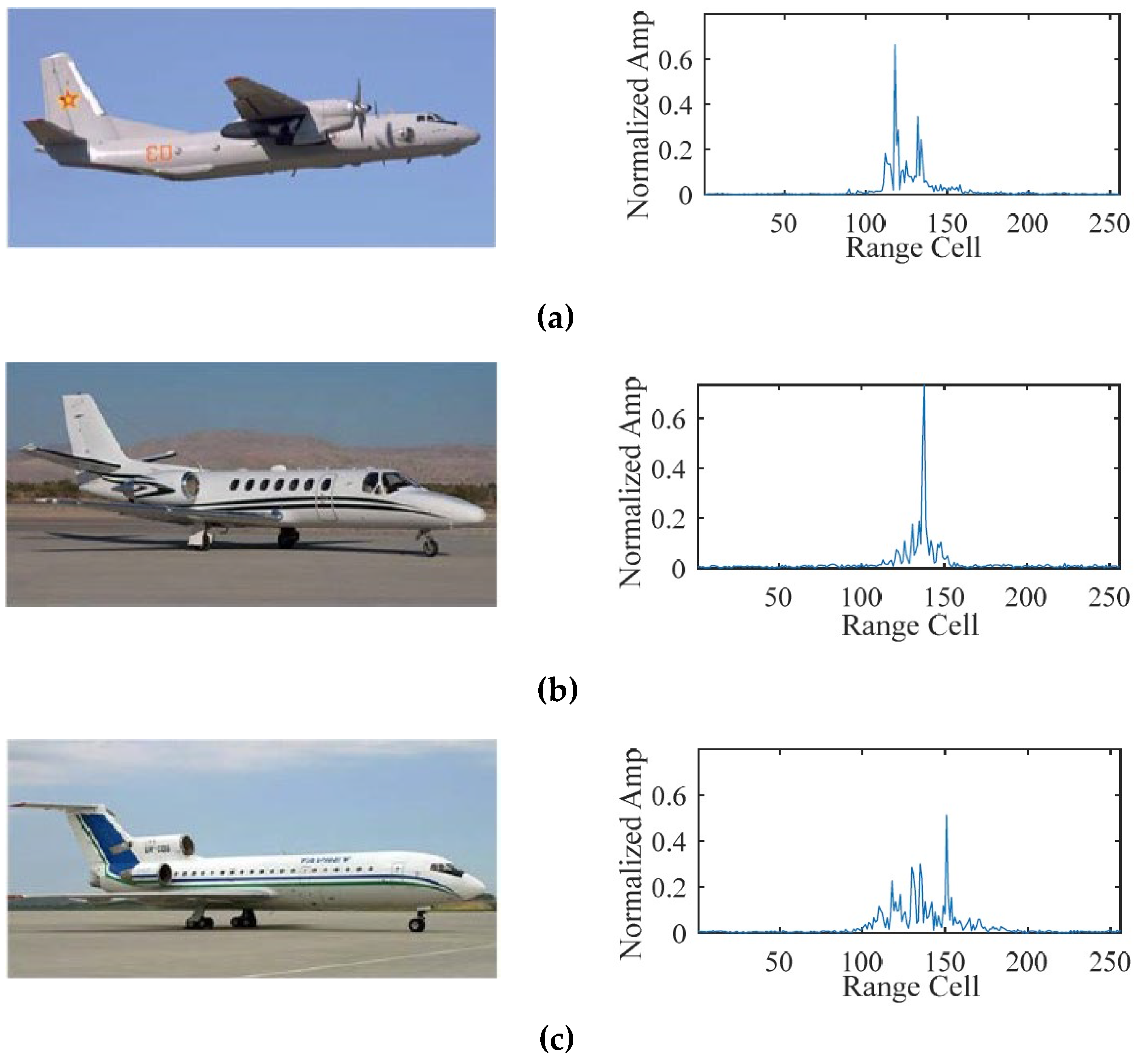
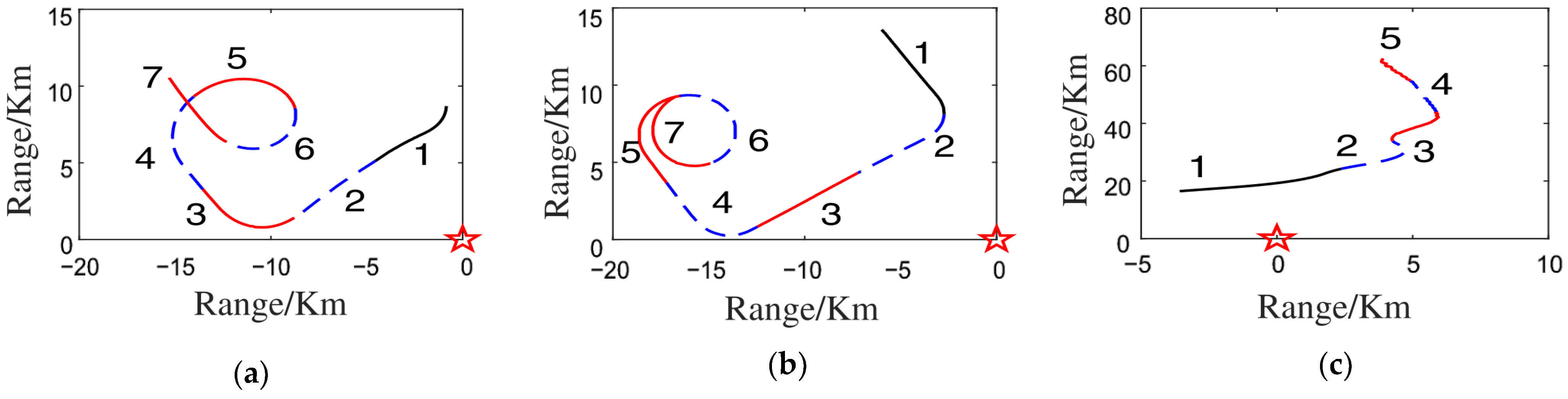
The high-resolution range profile (HRRP) of a target represents the 1D projection of its scattering centers along the radar line of sight (LOS), as shown in Figure 1. Compared with the 2D inverse synthetic aperture radar (ISAR) image, the HRRP is easier to acquire, store, and process. Moreover, it contains abundant structural signatures of the target such as the shape, size, and location of the main parts. Currently, automatic radar target recognition based on HRRP has received increasing attention in the radar automatic target recognition (RATR) community [1,2,3,4,5].

HRRP recognition can be achieved by traditional methods and deep learning. Traditional HRRP recognition methods [6,7,8,9,10,11,12] mainly depend on manually designed features and classifiers, which require extensive domain knowledge. Additionally, their heavy computational burden and poor generalization performance hinder practical application. Recently, HRRP recognition based on deep learning has avoided the tedious process of feature design and selection, and achieved much better performance than traditional approaches [13,14,15,16,17,18,19,20,21,22].

In real-world situations, however, the existence of strong noise will lead to a low signal-to-noise ratio (SNR) and hinder effective feature extraction. To deal with this issue, the available methods implement denoising firstly and then carry out feature extraction and recognition [19]. In terms of deep neural networks, however, such two-stage processing prohibits end-to-end training, resulting in complicated processing as well as long operational time. Furthermore, decoupling denoising from recognition ignores the potential requirements for noise suppression and signal extraction when fulfilling effective recognition. Therefore, it is natural to study the network structure integrating denoising and recognition to boost the performance and efficiency.

Traditional HRRP recognition methods are mainly divided into three categories: (1) feature domain transformation [6,7,8]; (2) statistical modeling [3,4,5,9,10]; and (3) kernel methods [11,12]. The first category obtains features in the transformation domain, e.g., the bispectra domain [6], by data projection, and then designs proper classifiers for HRRP recognition. The over-dependency on the prior knowledge, however, induces degraded performance and robustness in complex scenarios where priors are improper or unavailable. The second category establishes statistical models by imposing specific distributions, e.g., Gaussian [5], on the HRRP, which may result in limited data description capability, optimization space, and generalization performance. The third category projects the HRRP to higher feature space through kernels. In order to obtain satisfying recognition and generalization performance, however, the kernels should be carefully designed, such as kernel optimization based on the localized kernel fisher criterion [12].

In recent years, deep learning [14] has received intensive attention in HRRP recognition. Unlike traditional methods that rely heavily on hand-designed features, methods based on deep learning are data-driven, i.e., they could extract features of the HRRP automatically, through typical structures such as the autoencoder (AE) [15,16], the convolutional neural network (CNN) [17,18,19,20], and the recurrent neural network (RNN) [21,22], etc. The proposed method belongs to deep learning. Constituted by the encoder and the decoder, the AE attempts to output a copy of the input data by reconstructing it in an unsupervised fashion. In particular, the encoded, i.e., compressed data in the middle, serves as the recognition feature, which is then fed into the classifier for recognition [15,16]. The traditional CNN [17] extracts hierarchical spatial features from the input by cascaded convolutional and pooling layers, whereas it fails to capture the temporal information [18,19,20]. In view of this, RNN [21] has sequential architecture to process the current input and historical information simultaneously, so that to capture the temporal information of the target. However, it assumes that both the target and noise regions contribute equally to HRRP recognition, which may result in limited performance [22].

Mimicking the human vision, the attention mechanism [23,24,25,26] captures long-term information and dependencies between input sequence elements by measuring the importance of the input to the output. Traditional attention models designed for HRRP recognition [27,28,29,30,31], such as the target-attentional convolutional neural network (TACNN) [28], the target-aware recurrent attentional network (TARAN) [29], and the stacked CNN–Bi-RNN (CNN–Bi-RNN) [30]. TACNN, which is based on CNN, fails to make full use of the temporal correlation of HRRP, whereas TARAN, which is based on RNN and its variants, has difficulties in network training, parallelization, and long-term memory representation. Furthermore, CNN–Bi-RNN fuses the advantages of CNN and RNN and uses an attention mechanism to adjust the importance of features. In recent years, self-attention [32], which relates different positions of a single sequence to compute a global representation, has achieved efficient and parallel sequence modeling and feature extraction. Specifically, it acquires the attention score by calculating the correlation between the query vector and the key vector, and then weights it to the value vector as the output. Since the self-attention mechanism explicitly models the interactions between all elements in the sequence, it is a feature extractor of global information with long-term memory. Moreover, the global random access of the self-attention mechanism facilitates the fast and parallel modeling of long sequences. For HRRP recognition, the self-attention is added before the convolutional long short-term memory (ConvLSTM) [33] in order to focus on more significant range cells. Because the main recognition structure, i.e., the LSTM, is still a variant of RNN, it fails to directly use the different importance between features for recognition. In addition, although the networks proposed by the existing methods have certain noise robustness, they fail to achieve better recognition results under the condition of low SNR.

Traditionally, HRRP denoising is implemented prior to feature extraction, and typical denoising methods include least mean square (LMS) [34,35], recursive least square (RLS) [36], and eigen subspace techniques [37], etc. Such techniques, however, rely heavily on domain expertise and fail to estimate the model-order (i.e., the number of signal components) accurately with low SNR. Recently, the generative adversarial network (GAN) has been introduced as a novel way to train a generative model, which could learn the complex distributions through the adversarial training between the generator and the discriminator [38]. Currently, GAN has been successfully applied to data generation [39,40], image conversion and classification [41,42], speech enhancement [43] and so on, which provides an effective way to blind HRRP denoising.

In a nutshell, the separated HRRP denoising and recognition processes, the inability to distinguish the contribution of the target regions and noisy regions during the feature extraction process, the incompetence in long-term/global dependency acquisition hinder effective recognition of the noisy HRRP. Specifically, the output of the classifier cannot be fed back to the denoising process, thus significant signal components may be suppressed during denoising. Meanwhile, the different intensity information of each component of the HRRP cannot be effectively utilized in the identification process. Therefore, it is natural to integrate the tasks of denoising and recognition through elaborately deigned deep architectures, under the guidance of proper loss.

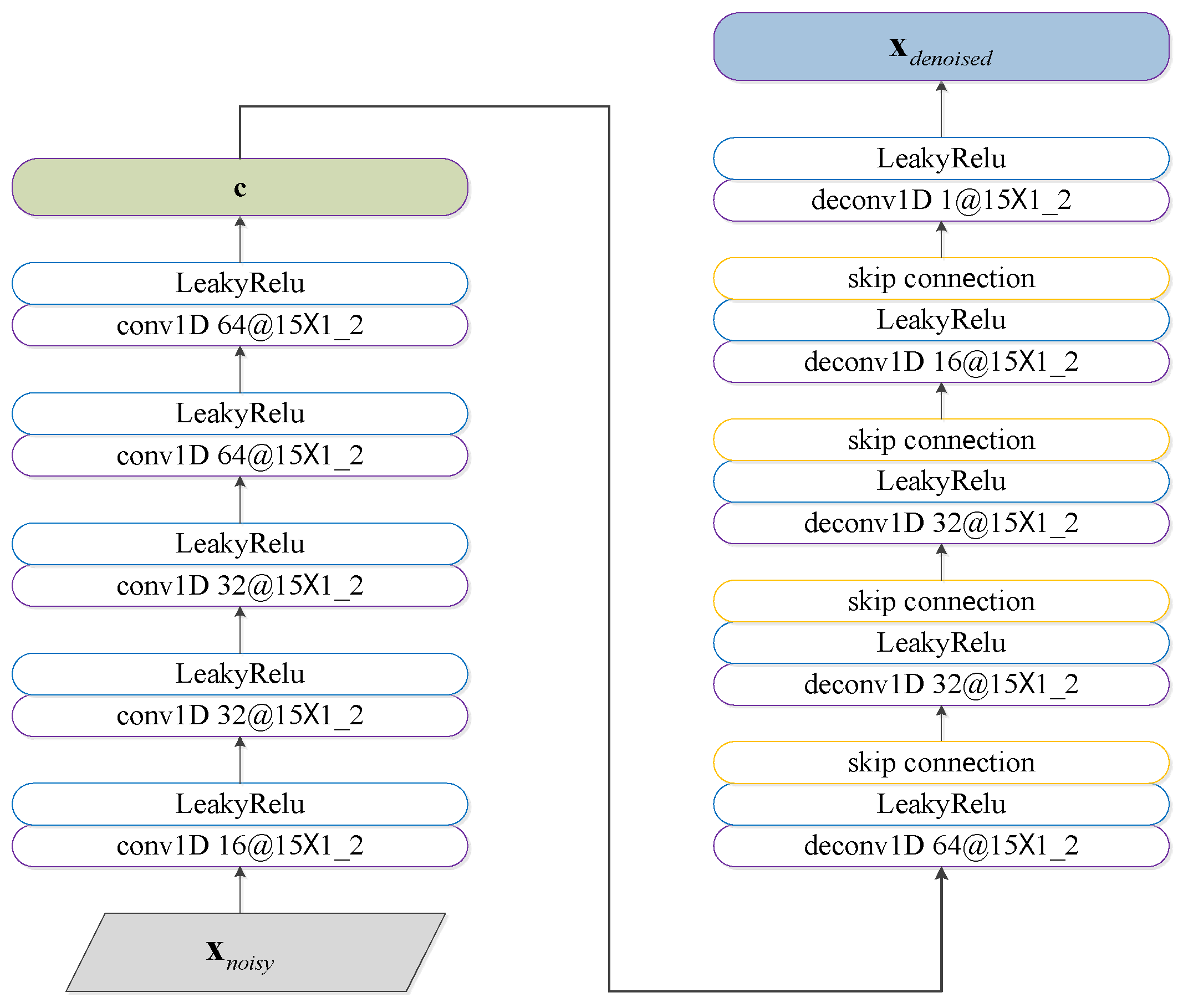
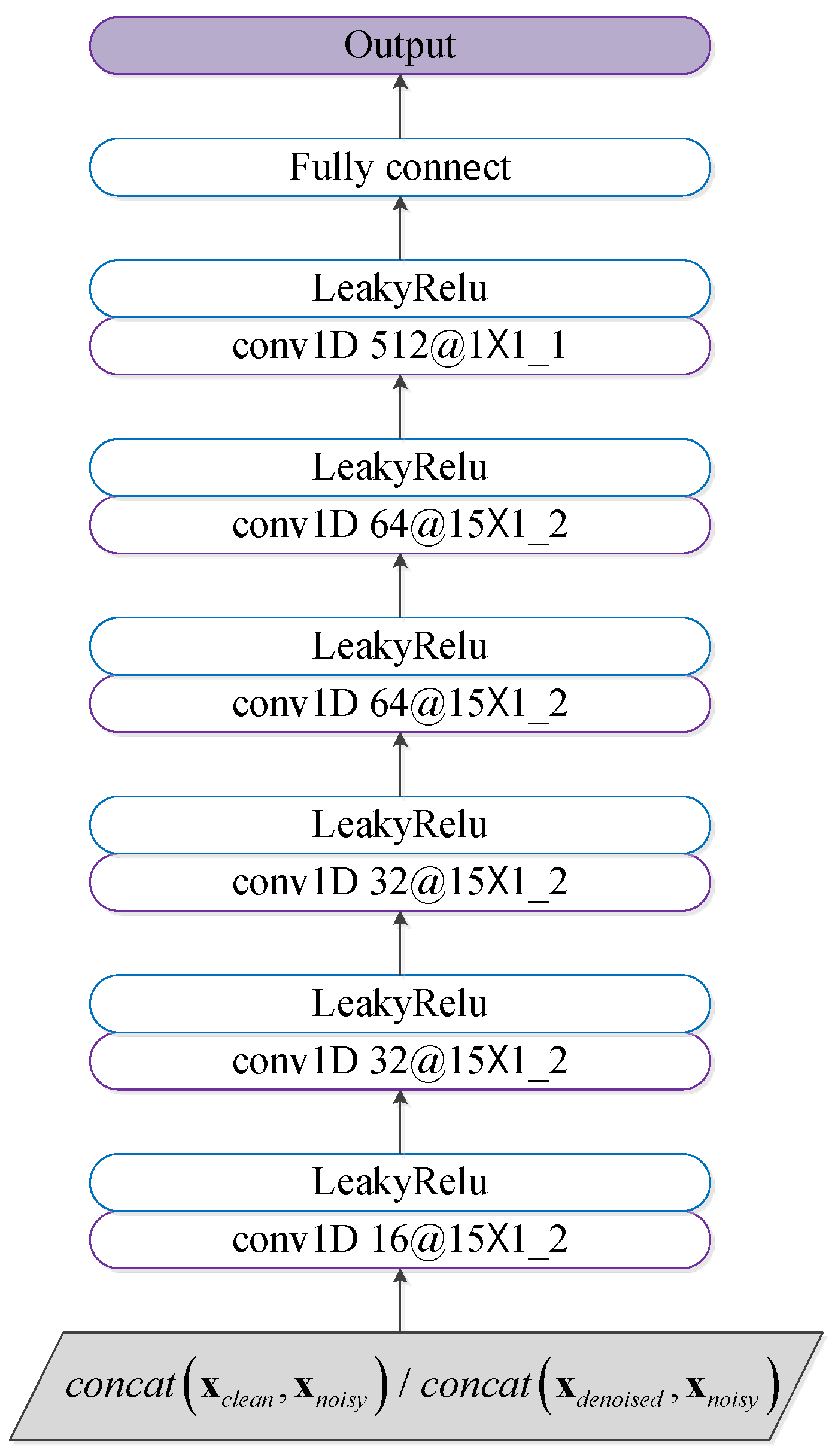
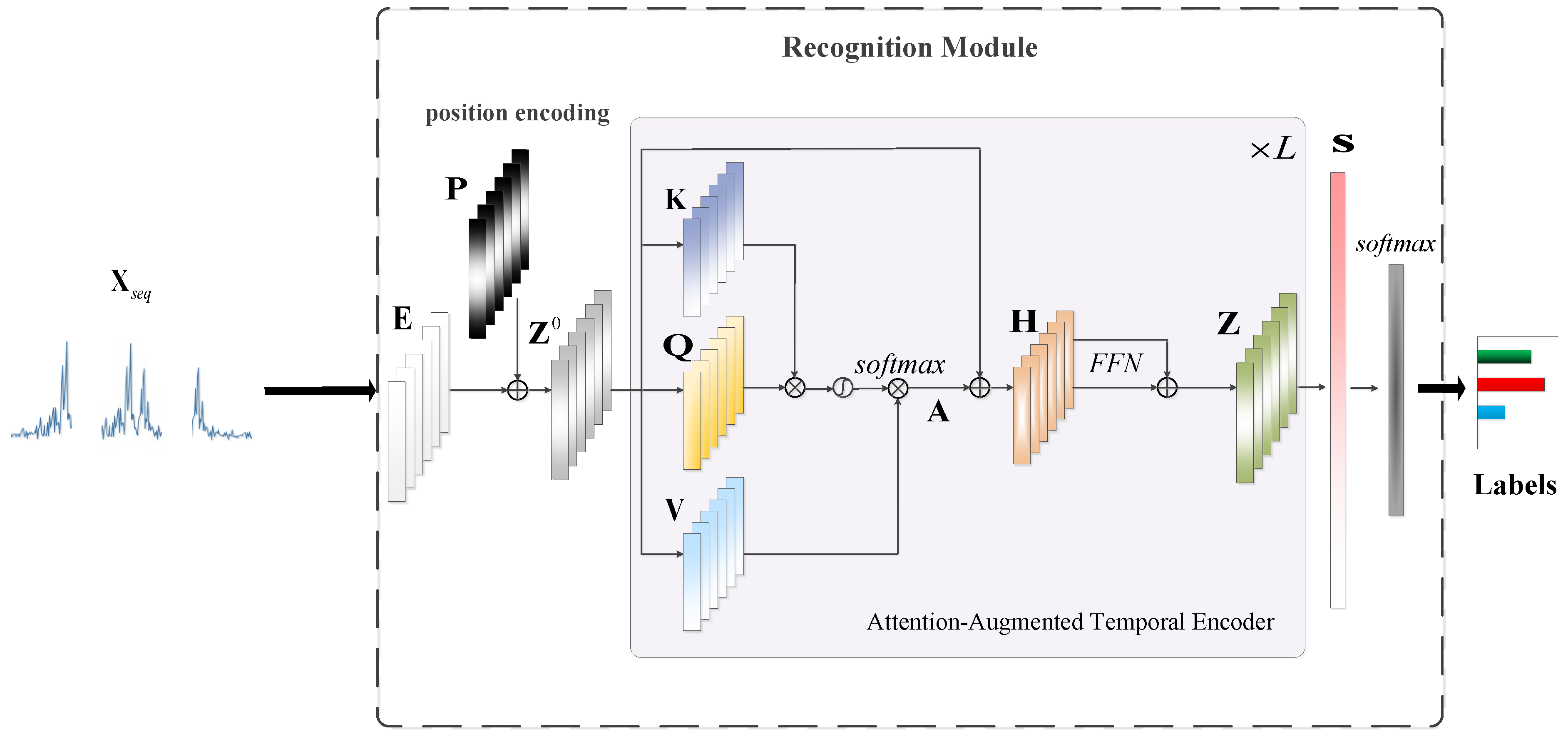
Aiming at the above issues, this paper proposes the integrated denoising and recognition network, namely, IDR-Net, to achieve effective HRRP denoising and recognition. The network consists of two modules, i.e., the denoising module and the recognition module. Specifically, the generator in the denoising module maps the noisy HRRP to the denoised one after adversarial training, which is then fed into the attention-augmented recognition module to output the target label. In particular, a new hybrid loss function is used to guide the denoising of HRRP. The main contributions of this paper include the following: (a) To tackle the issue that separated HRRP denoising and recognition hinder end-to-end training and may suppress signal components that are significant for recognition, an integrated denoising and recognition model, i.e., the IDR-Net is designed, denoising the low SNR HRRP through the denoising module and outputs the category label through the recognition module. To the best of our knowledge, our method integrates denoising and recognition for the first time, realizing end-to-end training, and achieving better recognition performance. (b) To tackle the issue of long-term and global dependency acquisition of HRRP, the recognition module adopts the attention-augmented temporal encoder with parallelized and global sequential feature extraction. In particular, the attention score is generated with emphasis on the important input data to weight the feature vector and facilitate recognition. (c) Propose a new hybrid loss, and for the first time in the recognition of HRRP using such a combination of denoising loss and classification loss as loss function. By these means, the recognition module is integrated with the generator, thereby reducing the information loss during denoising, and enhancing the inter-class dissimilarity.

The remainder of this paper is organized as follows: Section 2 discusses the related work, including the modelling of HRRP and the basic principles of GAN. Section 3 provides the detailed structure of the proposed IDR-Net. Section 4 presents the data set and experimental results with detailed analysis. Finally, Section 5 concludes this paper and discusses the future work.

2. Modeling and Related Work

2.1. HRRP Modeling

The high-resolution range profile (HRRP) is a 1-D signature of an object, which could represent the time domain response of a target to a high-range resolution radar pulse [13]. The complex valued HRRP of the target of the $n$th pulse can be expressed as

$$x_C\left(n\right)=e^{j\theta \left(n\right)}{\left[{\tilde{x}}_1\left(n\right),{\tilde{x}}_2\left(n\right),\dots {\tilde{x}}_M\left(n\right)\right]}^T$$

(1)

where $\theta \left(n\right)$ is the initial phase induced by translation. For the $m$th, $m\in \left[1,M\right]$, range cell, ${\tilde{x}}_m\left(n\right)={\displaystyle {\sum }_{p=1}^P{\sigma }_{mp}{e}^{j{\varphi }_{mp}\left(n\right)}}$ is the amplitude, where $P$ is the number of scattering centers; ${\sigma }_{mi}$ is the radar cross section of the $p$th scattering center; and ${\varphi }_{mp}\left(n\right)$ is the phase induced by the rotation of the $p$th scattering center. In addition, $T$ denotes vector transpose. Then, we obtain the real-valued HRRP by taking the modulus of $x_C\left(n\right)$, i.e.,

$$x\left(n\right)={\left[\left|{\tilde{x}}_1\left(n\right)\right|,\left|{\tilde{x}}_2\left(n\right)\right|,\dots ,\left|{\tilde{x}}_M\left(n\right)\right|\right]}^T$$

(2)

Generally, the HRRP is characterized by: (1) translation sensitivity; (2) amplitude sensitivity; and (3) aspect sensitivity. Specifically, the translational motion of the target will lead to unknown shifts among HRRPs along the range/temporal dimension; and the variation of the distance between the target and radar will cause amplitude fluctuation. Moreover, each scattering center has its own amplitude and phase characteristics, and these are combined as vectors to provide a net amplitude and phase return in the associated range cell, i.e., ${\tilde{x}}_m\left(n\right)$. These interference effects between scattering centers can give rise to rapid changes of the HRRP with aspect angle. To alleviate the sensitivities discussed above, we perform HRRP alignment and normalization, and then generate the training set utilizing HRRPs with various aspect angles.

2.2. GAN

GAN is a deep learning framework for estimating the generative models via adversarial training [38], which could sidestep the difficulty in approximating many intractable probabilistic computations. In general, a GAN consists of two adversarial models: a generator $G$ to capture the data distribution, and a discriminator $D$ to estimate the probability that a sample comes from the training data rather than $G$. That is to say, $G$ to generate samples close to the real samples, making the discriminator $D$ cannot distinguish them; at the same time, $D$ attempts to distinguish real samples from generated ones.

Both $G$ and $D$ could be non-linear mapping function, e.g., the deep neural network, and are trained following the two-player min-max game with the value function:

$$\underset{G}{\min } \underset{D}{\max }{V}_{GAN}\left(D,G\right)={\mathbb{E}}_{x~p_{data}\left(x\right)}\left[\log D\left(x\right)\right]+{\mathbb{E}}_{z~p_z\left(z\right)}\left[\log \left(1-D\left(G\left(z\right)\right)\right)\right]$$

(3)

where $\mathbb{E}\left[\cdot \right]$ is the expectation; $x$ is the sample comes from real distribution $p_{data}\left(x\right)$; and $z$ is the noise comes from latent distribution $p_z\left(z\right)$. By minimizing $\log \left(1-D\left(G\left(z\right)\right)\right)$, parameters of $G$ are adjusted to map $z$ into a new sample which is expected to have distribution $p_g$. Ideally, $p_g$ should be as close to $p_{data}$ as possible. By maximizing $\log D\left(x\right)$, parameters of $D$ are adjusted to distinguish the generated samples from the true ones. In practice, $G$ and $D$ are trained alternatively until convergence.

Traditional GAN is an unconditioned generative model, that is, there is no control on modes of the data being generated. In view of this, the conditional GAN (CGAN) [44] conditions the model on addition information and directs the data generation process. Specifically, it performs the conditioning by feeding the extra information $y$ to $G$ and $D$ in the training process. Then, the objective function becomes

$${\mathcal{L}}_{CGAN}\left(D,G\right)={\mathbb{E}}_{x~p_{data}\left(x\right)}\left[\log D\left(x|y\right)\right]+ {\mathbb{E}}_{z~p_z\left(z\right)}\left[\log \left(1-D\left(G\left(z|y\right)\right)\right)\right]$$

(4)

Currently, CGAN has been successfully applied to style transformation, such as image denoising [45] and image-to-image translation [46].

3. Network Structure

This section introduces the structure of IDR-Net, which consists of the denoising module and the recognition module. Firstly, the denoising module implements HRRP denoising through the generator. Then, the denoised HRRP is fed into the recognition module, which calculates the attention weights, extracts the features, and outputs the classification label. The framework of IDR-Net is shown in Figure 2, and the detailed structures will be introduced in Section 3.1, Section 3.2 and Section 3.3.

3.1. The Denoising Module

The denoising module treats HRRP denoising as a style transformation problem of converting the noisy HRRP into clean HRRP. For this purpose, the generator $G$ and the discriminator $D$ are designed according to the dimensionality of HRRP and trained with conditional information. Specifically, the generator $G$ maps the noisy HRRP $x_{noisy}$ to denoised HRRP $x_{denoised}$, and the discriminator $D$ distinguishes $x_{denoised}$ from the real noise-free HRRP $x_{clean}$. Below, we will discuss detailed structures of $G$ and $D$.

3.1.1. The Generator

According to the principles of GAN, the output of the generator $G$, i.e., $x_{denoised}$, should be resemble to the real noise-free HRRP $x_{clean}$ as closely as possible, so that the discriminator $D$ cannot distinguish $x_{denoised}$ from $x_{clean}$. In the IDR-Net, the non-linear mapping from $x_{noisy}$ to $x_{denoised}$ is achieved by an encoder and a decoder with symmetrical structures, as shown in Figure 3. For instance, “conv1D 16@15 1_2” denotes 1-D convolution with kernel size of 15 and stride size of 2, whereas “deconv1D 64@15 1_2” denotes deconvolution with kernel size of 15 and stride size of 2. In terms of HRRP denoising, the kernel size is set to $15\times 1$ with 2 stride sizes for each convolutional layer. The dimension of the input is $256\times 1$, and the dimension of the output feature map of each layer are $256\times 1$, $128\times 16$, $64\times 32$, $32\times 32$, $16\times 64$, and $8\times 64$, respectively. Then, the output $c$ of the last layer in the encoder is fed into the decoder, where the dimensions of the output of each layer is $16\times 64$, $32\times 32$, $64\times 32$, $128\times 16$, and $256\times 1$, respectively. The last layer outputs the denoised HRRP $x_{denoised}$.

As illustrated in the upper left part of the training process in Figure 2, the generator connects the output of each encoding layer and the output of the symmetrical decoding layer along the channel dimension through skip connection. By this means, it directly transfers the low-level features to the decoder without compression and facilitates gradient propagation.

3.1.2. The Discriminator

In the discriminator $D$, the noise-free HRRP $x_{clean}$ and $x_{denoised}$ are concatenated with the same noisy signal $x_{noisy}$, respectively, to obtain $\left[x_{clean},x_{noisy}\right]$ and $\left[x_{denoised},x_{noisy}\right]$. Conditioned by $x_{noisy}$, these vectors are then adopted as the real and generated samples, respectively, and fed into the network, as shown by the lower part of the training process of Figure 2. By introducing the conditional information $x_{noisy}$, we increase the similarity between the real samples and the generated ones, thereby facilitating the initial training stage of the network. That is, the outputs of $G$ become closer to the real samples, and the capability of distinguishing the real samples from the generated ones is enhanced for $D$.

As shown in Figure 4, the discriminator is composed of a series of 1D convolutional layers and fully connected layers, which has certain robustness to feature position. The size and number of the first five convolutional kernels are the same as those of the encoder in $G$. Moreover, LeakyReLU [45] with non-zero derivative is added to each convolutional layer, and the dimensions of the output feature maps are $128\times 16$, $64\times 32$, $32\times 32$, $16\times 64$, and $8\times 64$, respectively. Then, a convolutional layer with kernel size of $1\times 1$ and stride size of 1 is utilized to flatten the 2D feature map into a 1D vector. Finally, the fully connected layer outputs a scalar to indicate whether the current sample is real or generated.

3.2. The Recognition Module

The recognition module determines the category label of the denoised sample $x_{denoised}$ given by $G$. To exploit the sequential information among range cells of a single HRRP, we slide a sampling window continuously with a fixed size to generate the HRRP sequence. As discussed in Section 1, the traditional attention mechanism is confined to the inherent order of the sequence, thereby only processing two adjacent time steps. Therefore, it is essentially a local perception model and is incompetent to capture the global relationship of the entire sequence in parallel. To deal with this issue, the recognition module captures the long-term dependence efficiently through the attention-augmented temporal encoder, as shown in Figure 5.

Considering an HRRP, the sequence $X_{seq}={\left[x_1,\cdots ,x_N\right]}^{\mathrm{T}}$ is generated by sliding the sampling window with length $d_w$ and step size $d_w/2$, where $x_s\in {ℝ}^{d_w}$, $s=1,\dots ,N$, and $N$ is the number of segments. Then, a weight matrix $W_{map}\in {ℝ}^{d_w\times d}$ maps $X_{seq}$ linearly to obtain the embedding vectors $E^0=\left[e_0^0;e_1^0;\dots ;e_N^0\right]$ satisfying the following conditions

$$E^0=X_{seq}{W}_{map}$$

(5)

where $d$ is the hidden size.

Considering the position invariance of the attention mechanism, a learnable position encoding $P\in {ℝ}^{N\times d}$ is added to $E^0$, so as to better capture the sequential features, i.e.,

$$Z^0=E^0+P$$

(6)

After that, the L-layer attention-augmented temporal encoder calculates the attention score from $Z^0$ on the temporal dimension. Assuming that the input of the ($l-1$)th layer $(l=1,\dots ,L)$ of the encoder is $Z^{l-1}\in {\mathbb{R}}^{N\times d}$, the key $K^l$, query $Q{ }^l$ and value $V^l$ of the $l$th layer are calculated as follows:

$$\begin{array}{l}{k}_n^l=LN\left(z_n^{l-1}\right)W_k^l\\ q_n^l=LN\left(z_n^{l-1}\right)W_q^l\\ v_n^l=LN\left(z_n^{l-1}\right)W_v^l\end{array}$$

(7)

where $k_n^l$, $q_n^l$, and $v_n^l$ are row vectors of $K^l$, $Q{ }^l$, and $V^l$, respectively; $z_n^{l-1}$ is the $n$th row of $Z^{l-1}$; $W_k^l$, $W_q^l$, and $W_v^{ l}\in {ℝ}^{d\times d}$ are dimension transformation matrices; and $LN\left(·\right)$ is the layer normalization for calculating the mean and variance on all layers of each input, i.e.,

$$LN\left(z\right)=\rho ·\frac{z-\mu }{\sqrt{{\sigma }^2+\xi }}+b$$

(8)

where $\rho$ and $b$ are variable parameters; $\mu$ is the mean value and ${\sigma }^2$ is variance; and $\xi$ is a small nonzero value.

The attention score of the $l$th layer $A^l\in {ℝ}^{N\times d}$ can be calculated by:

$$A^l=\mathrm{softmax}\left(\frac{Q^l{\left(K^l\right)}^T}{\sqrt{d}}\right)V^l$$

(9)

To accelerate convergence, the residual $Z^{l-1}$ is added to $A^l$ and layer normalization is performed:

$$H^l=LN\left(A^l+Z^{l-1}\right)$$

(10)

Then, it is fed into a feedforward neural network (FFN), i.e.,

$$FFN\left(H^l\right)=\mathrm{ReLU}\left(H^l{W}_1\right)W_2$$

(11)

where $\mathrm{ReLU}(·)$ is the rectified linear unit [47,48]; $W_1\in {ℝ}^{d\times d_f}$, $W_2\in {ℝ}^{d_f\times d}$ are weight matrixes in FFN and $d_f$ is the corresponding dimension.

Furthermore, we add $H^l$ to (12) and perform layer normalization to obtain $Z^l\in {ℝ}^{N\times d}$:

$$Z^l=LN\left(FFN\left(H^l\right)+H^l\right)$$

(12)

After the L-layer encoder, $Z^L$ is vectorized into a feature vector $s\in {ℝ}^{1\times \left(N\times d\right)}$. Finally, the category label $y\in {ℝ}^{1\times K}$ is given by

$$y=\mathrm{soft}\max \left(\left(s{\mathbf{W}}_1^{\prime }\right){\mathbf{W}}_2^{\prime }\right)$$

(13)

where $K$ is the number of target categories; ${\mathbf{W}}_1^{\prime }\in {ℝ}^{\left(N\times d\right)\times d_f^{\prime }}$ and ${\mathbf{W}}_2^{\prime }\in {ℝ}^{d_f^{\prime }\times K}$ are the weights of fully connected layers with dimension $d_f^{\prime }$.

3.3. Construction of the Hybrid Loss

Traditional methods implement HRRP denoising and recognition separately, under the guidance of different losses. Such manipulation may lose important signal components beneficial to recognition. In view of this, we introduce the recognition loss to the value function of GAN and design the hybrid loss for integrated training of the IDR-Net. By this means, the recognition module is associated with the generator in the training process, thereby boosting the HRRP denoising, feature extraction, and recognition performance.

Since the generator and discriminator are trained alternatively, this paper expresses the losses of $G$ and $D$ in the denoising module separately as

$$\underset{G}{\min } {\mathcal{L}}_{G-loss}\left(D,G\right)={\mathcal{L}}_{base}+{\lambda }_{GP}\cdot {\mathcal{L}}_{GP}+{\rho }_1\cdot {\mathcal{L}}_{l_1}+{\rho }_2\cdot {\mathcal{L}}_{l_2}+\beta \cdot {\mathcal{L}}_{class}$$

(14)

$$\underset{D}{\min } {\mathcal{L}}_{D-loss}\left(D,G\right)=-\left({\mathcal{L}}_{base}+{\lambda }_{GP}\cdot {\mathcal{L}}_{GP}+{\rho }_1\cdot {\mathcal{L}}_{l_1}+{\rho }_2\cdot {\mathcal{L}}_{l_2}\right)$$

(15)

which are composed of the CGAN loss ${\mathcal{L}}_{base}$; the gradient penalty term ${\mathcal{L}}_{GP}$; the regularization terms ${\mathcal{L}}_{l_1}$ and ${\mathcal{L}}_{l_2}$; and the recognition loss ${\mathcal{L}}_{class}$. Moreover, ${\lambda }_{GP}$, ${\rho }_1$, ${\rho }_2$, and $\beta$ denote the corresponding coefficients. Below, each term will be discussed in detail.

To facilitate sample generation, i.e., HRRP denoising, we introduce the supervised learning strategy by adding $x_{noisy}$ to the loss function of GAN. Then, the CGAN loss is expressed as:

$${\mathcal{L}}_{base}={\mathbb{E}}_{x_{clean}}\left[D\left(x_{clean}|x_{noisy}\right)\right]-{\mathbb{E}}_z\left[D\left(G\left(z|x_{noisy}\right)\right)\right]$$

(16)

where $G\left(\cdot \right)$ denotes the generated samples, and $D\left(\cdot \right)$ denotes the discriminative score.

To avoid gradient explosion or vanishing and obtain a well-trained model, the gradient penalty term ${\mathcal{L}}_{GP}$ is designed as

$${\mathcal{L}}_{GP}={\mathbb{E}}_{\tilde{x}}\left[{\left({‖{\nabla }_{\tilde{x}}D\left(\tilde{x}\right)‖}_2-1\right)}^2\right]$$

(17)

In addition, ${\mathcal{L}}_{l_1}$ and ${\mathcal{L}}_{l_2}$ measure the similarity between the denoised sample and the clean one, i.e.,

$${\mathcal{L}}_{l_1}={\mathbb{E}}_{x_{noisy},x_{clean}}\left[{\Vert G\left(x_{noisy}\right)-x_{clean}\Vert }_1\right]$$

(18)

$${\mathcal{L}}_{l_2}={\mathbb{E}}_{x_{noisy},x_{clean}}\left[{‖G\left(x_{noisy}\right)-x_{clean}‖}_2\right]$$

(19)

In particular, the recognition loss ${\mathcal{L}}_{class}$ is added to the loss of $G$, which is expressed as

$${\mathcal{L}}_{class}=-{\mathbb{E}}_{X_{seq}}\left[{\displaystyle \sum _{k=1}^K{t}_k\ln y_k}\right]$$

(20)

where $t_k$ is the $k$th entry of the true label $t$, and $y_k$ is the $k$th entry of the predicted label $y$.

By omitting the irrelevant terms in (14) and (15), this paper finally obtains the losses of the generator and the discriminator of the IDR-Net, i.e.,

$$\underset{G}{\min } {\mathcal{L}}_{G-loss}\left(D,G\right)=-{\mathbb{E}}_z\left[D\left(G\left(z|x_{noisy}\right)\right)\right]+\lambda \left[\alpha {\mathcal{L}}_{l_1}+\left(1-\alpha \right){\mathcal{L}}_{l_2}\right]+\beta {\mathcal{L}}_{class}$$

(21)

$$\underset{D}{\min } {\mathcal{L}}_{D-loss}\left(D,G\right)={\mathbb{E}}_z\left[D\left(G\left(z|x_{noisy}\right)\right)\right]-{\mathbb{E}}_{x_{clean}}\left[D\left(x_{clean}|x_{noisy}\right)\right]+{\lambda }_{GP}{\mathcal{L}}_{GP}$$

(22)

where $\lambda$ is a regularization coefficient; and $\alpha \in \left(0,1\right)$ adjusts the proportion of ${\mathcal{L}}_{l_1}$ and ${\mathcal{L}}_{l_2}$ satisfies,

$$\alpha =\frac{{\rho }_1}{\lambda }$$

(23)

4. Experiments

4.1. Data Sets and Pre-Processing

In this section, we adopt the measured HRRPs of three types of aircraft, i.e., An-26, Cessna Citation S/II, and Yak-42, to design the experiments of network validation and performance analysis. The optical images and typical HRRPs are illustrated in Figure 6, and the size is listed in Table 1. Projections of the flight paths on the ground plane is illustrated in Figure 7, with radar located at the origin (0, 0). The radar pulse repetition frequency is 400 Hz, the bandwidth is 400 MHz, and the range resolution is 0.375 m. The echoes are divided into several segments, and the corresponding flight paths are indicated by integers ranging from 1 to 7, the number of samples for each data segment is listed in Table 2.

Table 1. Parameters of the aircraft.

Aircraft	Length (m)	Width (m)	Height (m)
An-26	23.80	29.20	9.83
Cessna Citation S/II	14.40	15.90	4.57
Yak-42	36.38	34.88	9.83

Table 1. Parameters of the aircraft.

Aircraft	Length (m)	Width (m)	Height (m)
An-26	23.80	29.20	9.83
Cessna Citation S/II	14.40	15.90	4.57
Yak-42	36.38	34.88	9.83

Figure 6. Optical images and typical HRRPs of (a) An-26; (b) Cessna Citation S/II; (c) Yak-42.

Figure 6. Optical images and typical HRRPs of (a) An-26; (b) Cessna Citation S/II; (c) Yak-42.

Figure 7. Projections of the trajectories on the ground. (a) An-26; (b) Cessna Citation S/II; (c)Yak-42.

Figure 7. Projections of the trajectories on the ground. (a) An-26; (b) Cessna Citation S/II; (c)Yak-42.

Table 2. The number of samples for each data segment of the three aircrafts.

Aircraft/No.	1	2	3	4	5	6	7
An-26	26,000	26,000	26,000	26,000	26,000	26,000	21,110
Cessna	26,000	26,000	26,000	26,000	26,000	26,000	26,000
Yak-42	26,000	26,000	26,000	26,000	17,950	—	—

Table 2. The number of samples for each data segment of the three aircrafts.

Aircraft/No.	1	2	3	4	5	6	7
An-26	26,000	26,000	26,000	26,000	26,000	26,000	21,110
Cessna	26,000	26,000	26,000	26,000	26,000	26,000	26,000
Yak-42	26,000	26,000	26,000	26,000	17,950	—	—

As a matter of routine [16,18,27,28,29,30], the training set is constructed by sampling the 5th and the 6th HRRP segments of An-26, the 6th and the 7th HRRP segments of Cessna Citation S/II, and the 2nd and the 5th HRRP segments of Yak-42, whereas the test set is constructed by sampling the rest HRRP segments. Moreover, the sampling interval is 20, and the number of training and test samples is 7398 and 16,656, respectively. Such settings could cover a wider range of aspect angles and mitigate the aspect sensitivity of HRRP. The division of the data set and number of samples is shown in

Table 3. Division of the data set and number of samples.

	An-26	Cessna	Yak-42	Total Sample No.
Segment No. for the training set	5, 6	6, 7	2, 5	7398
Segment No. for the test set	1, 2, 3, 4, 7	1, 2, 3, 4, 5	1, 3, 4	16,656

.

For the translation sensitivity, we align the samples by calculating the centroid of each HRRP [49], which is assumed to be constant in a short observation time. To eliminate the amplitude sensitivity, the $l_2$-norm normalization is implemented to each HRRP through

$$x_{l_2}=\frac{x}{{‖x‖}_2}$$

(24)

4.2. Training and Testing Process

We train the generator, the recognition module, and the discriminator of the IDR-Net alternately using the losses described in (21) and (22). Specifically, we calculate the gradients through back-propagation [50] and update the network parameters through the root mean square prop (RMSprop) gradient descent [51]. Such method can adaptively adjust the learning rate and has a faster descending speed than conventional methods. The main steps include:

$$\mathbb{E}{\left[g^2\right]}_k=\left(1-\phi \right)g_k^2+\phi \mathbb{E}{\left[g^2\right]}_{k-1}$$

(25)

$${\theta }_{k+1}={\theta }_k-\frac{\eta }{\sqrt{\mathbb{E}{\left[g^2\right]}_k+\delta }}\odot g_k$$

(26)

where $k$ is the index of iterations; ${\theta }_k$ is the set of network parameters at the $k$th iteration; $g_k=\frac{\partial \mathcal{L}}{\partial {\theta }_k}$ is the partial derivative of the loss $\mathcal{L}$ with respect to ${\theta }_k$; $\phi$ is the momentum coefficient; $\eta$ is the learning rate; $\delta$ is a small positive number to avoid the zero devisor; and $\odot$ is the dot product.

During training, the network is trained using noise-added measured data. The detailed training process of the IDR-Net is shown in Algorithm 1, where ${\theta }_k^G$, ${\theta }_k^D$, and ${\theta }_k^R$ represent the parameter sets of the generator $G$, the discriminator $D$, and the recognition module, respectively, at the $k$th iteration; and $x_k$ represents the output of the generator $G$.

Algorithm 1. Iterative alternating training process of the IDR-Net

1. Initialize:$k=0$,${\theta }_0^G$,${\theta }_0^D$,${\theta }_0^R$,$iter$,$x_0$

2. For$k=1:iter$

$\mathrm{Fix}$, update ${\theta }_k^D$ by (22) (26);

$\mathrm{Fix}$, update ${\theta }_k^G$ by (22) (26), $G$ generate $x_k$;

Feed $x_k$ into the recognition module, update ${\theta }_k^R$ by (20) (26);

Judge convergence;

End

3. Save model parameters

Additionally, the number of neurons in the fully connected layer in $D$ is 8; the length of the sliding window in the recognition module is 6; the number of layers in the attention-augmented temporal encoder is 5; and $d$ is set to 128. The detailed description of the hyperparameters is shown in

Table 4. Hyperparameters of training the IDR-Net.

Parameter	$\mathit{\eta }$	$\mathit{\alpha }$	$\mathit{\beta }$	$\mathit{\lambda }$	Batch Size	Epochs
Value	0.0002	0.5	0.015	160	256	600

. These parameters are determined empirically, making the IDR-Net perform better.

In the testing process, as shown in the lower part of Figure 2, we fix weights of $G$ and the recognition module, feed the noisy test sample to $G$, and then obtain the category label from the recognition module.

The IDR-Net is implemented based on the TensorFlow software, and the training and testing phases are implemented by a NVIDIA GTX 1080Ti GPU.

4.3. Recognition Results

In terms of the original HRRPs of the three aircrafts, we treat them as noise-free samples and generate the noisy training and test samples by adding Gaussian noise. Then, it implements preprocessing following the steps introduced in Section 4.1. Given SNR of 5 dB, 10 dB, and 15 dB, the confusion matrix, overall accuracy (OA), and per-class accuracy (PA) of the IDR-Net on the noisy test sets are shown in

Table 5. Recognition results of the IDR-Net on test sets.

SNR	T/P	An-26	Cessna	Yak-42	All	PA (%)
5 dB	An-26	3729	1488	1039	6256	59.61%
	Cessna	845	5605	50	6500	86.23%
	Yak-42	238	9	3653	3900	93.67%
	OA(%)		—			77.97%
10 dB	An-26	5187	500	569	6256	82.91%
	Cessna	1240	5252	8	6500	80.80%
	Yak-42	126	5	3769	3900	96.64%
	OA(%)		—			85.30%
15 dB	An-26	5464	452	340	6256	87.34%
	Cessna	1063	5432	5	6500	83.57%
	Yak-42	58	7	3835	3900	98.33%
	OA(%)		—			88.44%

. Each column of the confusion matrix denotes the true category label, whereas each row denotes the predicted label. The recognition accuracy is 77.97%, 85.30%, and 88.44%, respectively, for SNR of 5 dB, 10 dB, and 15 dB, respectively. Moreover, the recognition accuracy of Yak-42 is higher than that of An-26 and Cessna Citation S/II aircraft, which may be due to the similar size and trajectories of An-26 and Cessna Citation S/II.

To evaluate the denoising performance, we calculate the root mean square error (RMSE) between the denoised and the noise-free HRRPs by:

$$\mathrm{RMSE}=\frac{1}{\sqrt{L}}{‖x_{denoised}-x_{clean}‖}_2$$

(27)

The smaller RMSE indicates better denoising performance. For the test sets with different SNR, the statistical histograms of the RMSE before and after denoising are shown in Figure 8. By comparing the images in the same column, we observe that the denoised histogram shifts to the left, demonstrating the effectiveness of the generator.

To explain the feature extraction ability of the IDR-Net explicitly, Figure 9 visualizes the deep features of the noisy test samples for SNR of 5 dB, 10 dB, and 15 dB, respectively, by applying the t-distributed stochastic neighbor embedding (t-SNE) [52] to the output of the fully connected layer in the recognition module. Specifically, the first row demonstrates the separability of the original noisy samples, whereas the second row demonstrates the separability of the denoised ones. The red, green, and blue markers represent features of the An-26, Cessna Citation S/II, and Yak-42 aircraft, respectively. It is observed that the separability of the three aircrafts is boosted after denoising and attention-augmented temporal feature extraction.

4.4. Ablation Study

To demonstrate the validity of the denoising module (including the generator and the discriminator), the integrated denoising and recognition architectures, and the hybrid loss, we design two models: (1) the recognition network, i.e., the IDR-Net without the denoising module; and (2) the two-stage network, which carries out HRRP denoising and recognition separately. Similar to the IDR-Net, we feed the noisy samples into the recognition network for training and testing, and the loss function is expressed as Equation (20).

The two-stage network performs HRRP denoising through the denoising module of the IDR-Net firstly. Then, it feeds the denoised HRRPs into the recognition network to obtain the class label. It is worth noting that the denoising module is trained firstly by the noisy samples and the corresponding noise-free samples, and the loss function satisfies

$$\underset{G}{\min } {\mathcal{L}}_{G-loss}\left(D,G\right)=-{\mathbb{E}}_z\left[D\left(G\left(z|x_{noisy}\right)\right)\right]+\lambda \left[\alpha {\mathcal{L}}_{l_1}+\left(1-\alpha \right){\mathcal{L}}_{l_2}\right]$$

(28)

$$\underset{D}{\min } {\mathcal{L}}_{D-loss}\left(D,G\right)={\mathbb{E}}_z\left[D\left(G\left(z|x_{noisy}\right)\right)\right]-{\mathbb{E}}_{x_{clean}}\left[D\left(x_{clean}|x_{noisy}\right)\right]+{\lambda }_{GP}{\mathcal{L}}_{GP}$$

(29)

Then, the weights of the generator are fixed, and the denoised samples together with their labels are adopted to train the recognition network with the loss function given in Equation (20).

Detailed configurations for the two models and the IDR-Net are listed in

Table 6. Configurations of the three models.

Function/Method	IDR-Net	Recognition-Net	Two-Stage
Denoising	√	—	√
Recognition	√	√	√
End to end	√	√	—
Hybrid loss function	√	—	—

, and the corresponding recognition accuracies are listed in

Table 7. Comparisons of the recognition accuracy for SNR of 5 dB, 10 dB, 15 dB.

Method/SNR	5 dB	10 dB	15 dB
Recognition network	76.20%	83.18%	86.56%
Two-stage network	74.26%	81.45%	85.85%
IDR-Net	77.97%	85.30%	88.44%

. It can be found that the IDR-Net achieves the highest recognition accuracy for SNR of 5 dB, 10 dB, and 15 dB.

Compared with the recognition network, the recognition accuracy of the IDR-Net is improved by about 2%, demonstrating the effectiveness of the denoising module. Because the denoising module and the recognition module are trained separately in the two-stage model, the denoised samples may lose the information beneficial to recognition. On the contrary, the IDR-Net achieves integrated denoising and recognition through the hybrid loss, so that the denoising module is guided to generate samples facilitate recognition. Therefore, the recognition accuracy of the IDR-Net is about 3% higher than that of the two-stage network.

4.5. Contrast Experiments

Although methods for HRRP recognition emerge in an endless stream in recent years, they either design two networks for denoising and recognition separately, such as the SMTRNet [19], or directly design networks which are not robust to noise, such as DPmTRNN [1] and RFRAN [31]. Below, we will compare the performance of the IDR-Net with traditional HRRP recognition methods and recently proposed methods with certain noise robustness, i.e., the linear support vector machine (LSVM) [27], the CNN [18], the TACNN [28], the TARAN [29], the CNN–Bi-RNN [30], and the class factorized complex variational auto-encoder (CFCVAE) [16]. Among them, the LSVM is a traditional kernel method, which has satisfactory recognition and generalization performance. The remaining methods are deep models. Specifically, the CNN could effectively extract the local structural information of the HRRP; the TACNN is an attention-augmented CNN, where the learned attention coefficients can better represent the importance of each local feature in the recognition task; the TARAN is an attention-augmented RNN which could capture the temporal dependence and consider the contributions of different range cells during feature extraction, the CNN–Bi-RNN fuses the advantages of CNN and RNN and uses an attention mechanism to adjust the importance of features; and the CFCVAE is a variant of AE, which improves the feature characterization ability through multiple class-decoders.

Comparisons of the recognition accuracies between the available models and the IDR-Net are listed in

Table 8. Comparisons of the recognition accuracy under different SNRs.

Model/SNR	5 dB	10 dB	15 dB
LSVM	47.00%	57.90%	61.00%
CNN	63.80%	66.20%	70.00%
TACNN	62.31%	71.47%	74.69%
TARAN	59.90%	60.50%	63.70%
CNN–Bi-RNN	68.06%	69.20%	74.72%
CFCVAE	70.35%	75.50%	81.22%
IDR-Net	77.97%	85.30%	88.44%

, where the proposed model achieves the highest recognition accuracy on the noisy test sets with different SNR. Because traditional recognition methods mainly utilize shallow models, they have limited data description capabilities. On the contrary, deep neural networks are data-driven and could extract hierarchical features conducive to HRRP recognition. As demonstrated by Table 8, the recognition accuracies of the deep models are significantly higher than traditional method. However, the CNN fails to calculate the sequential relationships, whereas the methods based on traditional attention cannot describe the global information of the HRRP sequence. To tackle these issues, the IDR-Net suppresses the impact of noise on HRRP feature extraction through the denoising module, and then designs the attention-augmented temporal encoder extract the global information in parallel, thereby effectively boosting the recognition accuracy and the robustness to noise.

5. Conclusions

To achieve integrated of denoising and recognition of HRRPs in low SNR scenarios, this paper proposes the IDR-Net, which converts the noisy HRRP to denoised HRRP though adversarial training, and realizes global relationship extraction through the self-attention mechanism. The hybrid loss is designed to preserve significant features beneficial to recognition during denoising and facilitate end-to-end training. The experimental results on the measured HRRP data have demonstrated that the IDR-Net has higher recognition accuracy and stronger robustness to noise than traditional methods.

In the future, we will focus on studying effective feature extraction and recognition of HRRP under complex conditions such as data deficiency and deformation, and on exploring sequential features for HRRP sequence recognition.

References

1. Chen, W.; Chen, B.; Peng, X.; Liu, J.; Yang, Y.; Zhang, H.; Liu, H. Tensor RNN with Bayesian nonparametric mixture for radar HRRP modeling and target recognition. IEEE Trans. Signal Process. 2021, 69, 1995–2009. [Google Scholar] [CrossRef]
2. Huang, T.; Chen, Y.; Yao, B.; Yang, B.; Wang, X.; Li, Y. Adversarial attacks on deep-learning-based radar range profile target recognition. Inf. Sci. 2020, 531, 159–176. [Google Scholar] [CrossRef]
3. Chen, J.; Du, L.; Guo, Y. Label constrained convolutional factor analysis for classification with limited training samples. Inf. Sci. 2021, 544, 372–394. [Google Scholar] [CrossRef]
4. Guo, D.; Chen, B.; Chen, W.; Wang, C.; Liu, H.; Zhou, M. Variational temporal deep generative model for radar HRRP target recognition. IEEE Trans. Signal Process. 2020, 68, 5795–5809. [Google Scholar] [CrossRef]
5. Du, L.; Chen, J.; Hu, J.; Li, Y.; He, H. Statistical modeling with label constraint for radar target recognition. IEEE Trans. Aerosp. Electron. Syst. 2020, 56, 1026–1044. [Google Scholar] [CrossRef]
6. Zhang, X.; Shi, Y.; Bao, Z. A new feature vector using selected bispectra for signal classification with application in radar target recognition. IEEE Trans. Signal Process. 2001, 49, 1875–1885. [Google Scholar] [CrossRef]
7. Du, L.; Liu, H.; Bao, Z.; Xing, M. Radar HRRP target recognition based on higher order spectra. IEEE Trans. Signal Process. 2005, 53, 2359–2368. [Google Scholar]
8. Zhang, X.; Wang, W.; Zheng, X.; Wei, Y. A novel radar target recognition method for open and imbalanced high-resolution range profile. Digit. Signal Process. 2021, 118, 103212. [Google Scholar] [CrossRef]
9. Cospey, K.; Webb, A. Bayesian gamma mixture model approach to radar target recognition. IEEE Trans. Aerosp. Electron. Syst. 2003, 39, 1201–1217. [Google Scholar]
10. Du, L.; Liu, H.; Bao, Z. Radar HRRP statistical recognition: Parametric model and model selection. IEEE Trans. Signal Process. 2008, 56, 1931–1944. [Google Scholar] [CrossRef]
11. Chen, B.; Yuan, L.; Liu, H.; Bao, Z. Kernel subclass discriminant analysis. Neurocomputing 2007, 71, 445–458. [Google Scholar] [CrossRef]
12. Chen, B.; Liu, H.; Bao, Z. A kernel optimization method based on the localized kernel fisher criterion. Pattern Recognit. 2008, 41, 1098–1109. [Google Scholar] [CrossRef]
13. Feng, B.; Chen, B.; Liu, H. Radar HRRP target recognition with deep networks. Pattern Recognit. 2017, 61, 379–393. [Google Scholar] [CrossRef]
14. LeCun, Y.; Bengio, Y.; Hinton, G. Deep learning. Nature 2015, 521, 436–444. [Google Scholar] [CrossRef]
15. Li, C.; Du, L.; Deng, S.; Sun, Y.; Liu, H. Point-wise discriminative auto-encoder with application on robust radar automatic target recognition. Signal Process. 2020, 169, 107385. [Google Scholar] [CrossRef]
16. Liao, L.; Du, L.; Chen, J. Class factorized complex variational auto-encoder for HRR radar target recognition. Signal Process. 2021, 182, 107932. [Google Scholar] [CrossRef]
17. LeCun, Y.; Bottou, L.; Bengio, Y.; Haffner, P. Gradient-based learning applied to document recognition. Proc. IEEE 1998, 86, 2278–2324. [Google Scholar] [CrossRef] [Green Version]
18. Wan, J.; Chen, B.; Xu, B.; Liu, H.; Jin, L. Convolutional neural networks for radar HRRP target recognition and rejection. EURASIP J. Adv. Signal Process. 2019, 2019, 1–17. [Google Scholar] [CrossRef] [Green Version]
19. Zhao, C.; He, X.; Liang, J.; Wang, T.; Huang, C. Radar HRRP target recognition via semi-supervised multi-task deep network. IEEE Access 2019, 7, 114788–114794. [Google Scholar] [CrossRef]
20. Guo, C.; He, Y.; Wang, H.; Jian, T.; Sun, S. Radar HRRP target recognition based on deep one-dimensional residual-inception network. IEEE Access 2019, 7, 9191–9204. [Google Scholar] [CrossRef]
21. Schuster, M.; Paliwal, K.K. Bidirectional recurrent neural networks. IEEE Trans. Signal Process. 1997, 45, 2673–2681. [Google Scholar] [CrossRef] [Green Version]
22. Zhang, Y.; Xiao, F.; Qian, F.; Li, X. VGM-RNN: HRRP sequence extrapolation and recognition based on a novel optimized RNN. IEEE Access 2020, 8, 70071–70081. [Google Scholar] [CrossRef]
23. Bahdanau, D.; Cho, K.; Bengio, Y. Neural machine translation by jointly learning to align and translate. arXiv 2014, arXiv:1409.0473. [Google Scholar]
24. Fu, J.; Zheng, H.; Mei, T. Look closer to see better: Recurrent attention convolutional neural network for fine-grained image recognition. In Proceedings of the IEEE International Conference on Computer Vision and Pattern Recognition (CVPR), Honolulu, HI, USA, 21–26 July 2017; pp. 4476–4484. [Google Scholar]
25. Xue, R.; Bai, X.; Cao, X.; Zhou, F. Sequential ISAR Target Classification Based on Hybrid Transformer. IEEE Trans. Geosci. Remote Sens. 2022, 60, 1–11. [Google Scholar] [CrossRef]
26. Yang, M.; Bai, X.; Wang, L.; Zhou, F. Mixed Loss Graph Attention Network for Few-Shot SAR Target Classification. IEEE Trans. Geosci. Remote Sens. 2022, 60, 1–13. [Google Scholar] [CrossRef]
27. Wan, J.; Chen, B.; Liu, Y.; Yuan, Y.; Liu, H.; Jin, L. Recognizing the HRRP by combining CNN and BiRNN with attention mechanism. IEEE Access 2020, 8, 20828–20837. [Google Scholar] [CrossRef]
28. Chen, J.; Du, L.; Guo, G.; Yin, L.; Wei, D. Target-attentional CNN for radar automatic target recognition with HRRP. Signal Process. 2022, 196, 108497. [Google Scholar] [CrossRef]
29. Xu, B.; Chen, B.; Wan, J.; Liu, H.; Jin, L. Target-aware recurrent attentional network for radar HRRP target recognition. Signal Process. 2019, 155, 268–280. [Google Scholar] [CrossRef]
30. Pan, M.; Liu, A.; Yu, Y.; Wang, P.; Li, J.; Liu, Y.; Lv, S.; Zhu, H. Radar HRRP target recognition model based on a stacked CNN–Bi-RNN with attention mechanism. IEEE Trans. Geosci. Remote Sens. 2022, 60, 1–14. [Google Scholar] [CrossRef]
31. Du, C.; Tian, L.; Chen, B.; Zhang, L.; Chen, W.; Liu, H. Region-factorized recurrent attentional network with deep clustering for radar HRRP target recognition. Signal Process. 2021, 183, 108010. [Google Scholar] [CrossRef]
32. Vaswani, A.; Shazeer, N.; Parmar, N.; Uszkoreit, J.; Jones, L.; Gomez, A.N.; Kaiser, L.; Polosukhin, I. Attention is all you need. In Proceedings of the International Conference on Neural Information Processing Systems (NIPS), Long Beach, CA, USA, 4–9 December 2017; pp. 5998–6008. [Google Scholar]
33. Zhang, L.; Li, Y.; Wang, Y.; Wang, J.; Long, T. Polarimetric HRRP recognition based on ConvLSTM with self-attention. IEEE Sens. J. 2021, 21, 7884–7898. [Google Scholar] [CrossRef]
34. Aggarwal, S.; Dwivedi, P.; Jagannatham, A.K. Fast block LMS and RLS-based parameter estimation and two-dimensional imaging in monostatic MIMO RADAR systems with multiple mobile targets. IEEE Trans. Signal Process. 2018, 66, 1775–1790. [Google Scholar]
35. Ma, Y.; Shan, T.; Zhang, Y.; Amin, M.G.; Tao, R.; Feng, Y. A novel two-dimensional sparse-weight NLMS Filtering scheme for passive bistatic radar. IEEE Geosci. Remote Sens. Lett. 2016, 13, 676–680. [Google Scholar] [CrossRef]
36. Zhu, X.; Zhang, X. Adaptive RLS algorithm for blind source separation using a natural gradient. IEEE Signal Process. Lett. 2002, 9, 432–435. [Google Scholar]
37. Zhou, F.; Wu, R.; Xing, M.; Bao, Z. Eigensubspace-based filtering with application in narrow-band interference suppression for SAR. IEEE Geosci. Remote Sens. Lett. 2007, 4, 75–79. [Google Scholar] [CrossRef]
38. Goodfellow, I.; Pouget-Abadie, J.; Mirza, M.; Xu, B.; Warde-Farley, D.; Ozair, S.; Courville, A.; Bengio, Y. Generative adversarial nets. In Proceedings of the International Conference on Neural Information Processing Systems (NIPS), Montreal, QC, Canada, 8–11 December 2014; Volume 2, pp. 2672–2680. [Google Scholar]
39. Zheng, Z.; Yang, X.; Yu, Z.; Zheng, L.; Yang, Y.; Kautz, J. Joint discriminative and generative learning for person re-identification. In Proceedings of the IEEE International Conference on Computer Vision and Pattern Recognition (CVPR), Long Beach, CA, USA, 15–20 June 2019. [Google Scholar]
40. Shi, L.; Liang, Z.; Wen, Y.; Zhuang, Y.; Huang, Y.; Ding, X. One-shot HRRP generation for radar target recognition. IEEE Geosci. Remote Sens. Lett. 2022, 19, 1–5. [Google Scholar] [CrossRef]
41. Zhu, J.; Park, T.; Isola, P.; Efros, A.A. Unpaired image-to-image translation using cycle-consistent adversarial networks. In Proceedings of the IEEE International Conference on Computer Vision (ICCV), Venice, Italy, 22–29 October 2017; pp. 2242–2251. [Google Scholar]
42. Zhu, L.; Chen, Y.; Ghamisi, P.; Benediktsson, J.A. Generative adversarial networks for hyperspectral image classification. IEEE Trans. Geosci. Remote Sens. 2018, 56, 5046–5063. [Google Scholar] [CrossRef]
43. Pascual, S.; Bonafonte, A.; Serra, J. SEGAN: Speech enhancement generative adversarial network. arXiv 2017, arXiv:1703.09452. [Google Scholar]
44. Mirza, M.; Osindero, S. Conditional generative adversarial nets. arXiv 2014, arXiv:1411.1784. [Google Scholar]
45. Chen, J.; Chao, H.; Yang, M. Image blind denoising with generative adversarial network based noise modeling. In Proceedings of the IEEE International Conference on Computer Vision and Pattern Recognition (CVPR), Salt Lake City, UT, USA, 18–23 June 2018. [Google Scholar]
46. Isola, P.; Zhu, J.; Zhou, T.; Efros, A.A. Image-to-image translation with conditional adversarial networks. In Proceedings of the IEEE/CVF Conference on Computer Vision and Pattern Recognition (CVPR), Honolulu, HI, USA, 21–26 July 2017; pp. 5967–5976. [Google Scholar]
47. Maas, A.L.; Hannun, A.Y.; Ng, A.Y. Rectifier nonlinearities improve neural network acoustic models. In Proceedings of the International Conference on Machine Learning (ICML), Atlanta, GA, USA, 16–21 June 2013. [Google Scholar]
48. Glorot, X.; Bordes, A.; Bengio, Y. Deep sparse rectifier neural networks. In Proceedings of the 14th International Conference on Artificial Intelligence and Statistics (AISTATS), Fort Lauderdale, FL, USA, 11–13 April 2011; Volume 15, pp. 315–323. [Google Scholar]
49. Itoh, T.; Sueda, H.; Watanabe, Y. Motion compensation for ISAR via centroid tracking. IEEE Trans. Aerosp. Electron. Syst. 1996, 32, 1191–1197. [Google Scholar] [CrossRef]
50. Rumelhart, D.; Hinton, G.E.; Williams, R.J. Learning representations by back-propagating errors. Nature 1986, 323, 533–536. [Google Scholar] [CrossRef]
51. Bera, S.; Shrivastava, V.K. Analysis of various optimizers on deep convolutional neural network model in the application of hyperspectral remote sensing image classification. Int. J. Remote Sens. 2020, 41, 2664–2683. [Google Scholar] [CrossRef]
52. van der Maaten, L.; Hinton, G. Visualizing data using t-SNE. J. Mach. Learn. Res. 2008, 9, 2579–2605. [Google Scholar]
Figure 1. Illustration of the HRRP of an airplane.
Remotesensing 14 05254 g001
Figure 2. The framework of the IDR-Net.
Remotesensing 14 05254 g002
Figure 3. Detailed structure of the generator.
Remotesensing 14 05254 g003
Figure 4. Detailed structure of the discriminator.
Remotesensing 14 05254 g004
Figure 5. Detailed structure of the recognition module.
Remotesensing 14 05254 g005
Figure 8. Statistical histograms of the RMSE before and after denoising. (ac): RMSE of the noisy test samples for SNR of 5 dB, 10 dB, and 15 dB; (df): RMSE of the denoised samples for SNR of 5 dB, 10 dB, and 15 dB.
Remotesensing 14 05254 g008
Figure 9. Comparisons of the visualized output features between (ac): original noisy test samples with SNR of 5 dB, 10 dB, 15 dB; and (df): denoised test samples with SNR of 5 dB, 10 dB, 15 dB.
Remotesensing 14 05254 g009