Article

Spatiotemporal Assessment of Satellite Image Time Series for Land Cover Classification Using Deep Learning Techniques: A Case Study of Reunion Island, France

by
Naik Nitesh Navnath
1,
Kandasamy Chandrasekaran
1,
Andrzej Stateczny
2,*,
Venkatesan Meenakshi Sundaram
3 and
Prabhavathy Panneer
4
1
Department of Computer Science and Engineering, National Institute of Technology Karnataka, Surathkal, Mangalore 575025, Karnataka, India
2
Department of Geodesy, Gdańsk University of Technology, Gabriela Narutowicza 11-12, 80-233 Gdańsk, Poland
3
Department of Computer Science and Engineering, National Institute of Technology Puducherry, Karaikal 609609, Puducherry, India
4
School of Information Technology and Engineering, Vellore Institute of Technology, Katpadi, Vellore 632014, Tamil Nadu, India
*
Author to whom correspondence should be addressed.
Remote Sens. 2022, 14(20), 5232; https://doi.org/10.3390/rs14205232
Submission received: 18 September 2022 / Revised: 8 October 2022 / Accepted: 11 October 2022 / Published: 19 October 2022

Abstract

:
Current Earth observation systems generate massive amounts of satellite image time series to keep track of geographical areas over time to monitor and identify environmental and climate change. Efficiently analyzing such data remains an unresolved issue in remote sensing. In classifying land cover, utilizing SITS rather than one image might benefit differentiating across classes because of their varied temporal patterns. The aim was to forecast the land cover class of a group of pixels as a multi-class single-label classification problem given their time series gathered using satellite images. In this article, we exploit SITS to assess the capability of several spatial and temporal deep learning models with the proposed architecture. The models implemented are the bidirectional gated recurrent unit (GRU), temporal convolutional neural networks (TCNN), GRU + TCNN, attention on TCNN, and attention of GRU + TCNN. The proposed architecture integrates univariate, multivariate, and pixel coordinates for the Reunion Island’s landcover classification (LCC). the evaluation of the proposed architecture with deep neural networks on the test dataset determined that blending univariate and multivariate with a recurrent neural network and pixel coordinates achieved increased accuracy with higher F1 scores for each class label. The results suggest that the models also performed exceptionally well when executed in a partitioned manner for the LCC task compared to the temporal models. This study demonstrates that using deep learning approaches paired with spatiotemporal SITS data addresses the difficult task of cost-effectively classifying land cover, contributing to a sustainable environment.

1. Introduction

Over the years, progressive development in modern Earth observation programs has assisted in monitoring the surface of the Earth by continuously delivering enormous amounts of satellite data. The high revisit period has immensely contributed to the production of SITS with an increased spatial resolution that represents an effective tool to monitor the transition on the surface of the Earth through time by providing enormous support in various applications. Satellite image time series (SITS) has been successfully applied in multiple applications such as ecology [1], farming and agricultural development [2], risk analysis health and mobility [3], devising schemes for the effective management of land [4], forest [5], and monitoring of natural habitat [6]. Our environment is frequently changing, necessitating constant improvements in land use and land cover (LULC) data to assist logical decision making. Land use defines the utilization of the land in a particular area, such as residential buildings, industrial sites, and agricultural regions. What physically exists on the surface of the Earth, such as water bodies, grasslands, and different kinds of forests, is called the land cover [7]. It is therefore critical to create highly effective and valuable strategies for obtaining LULC information in an automated and intelligent manner. There is a higher probability of land cover being present in land use, which becomes challenging to identify the land cover with remote sensing technology [8].
LULC data are crucial in multiple applications such as the administration of regional plans, urban development, monitoring, as well as the management of the environment in the domain of geospatial data analysis [9]. Climate change and disaster risk management are among the biggest challenges for environmental assessment and can be tackled through spatiotemporal properties exhibited by the LULC information [10]. In recent years, multitemporal images have been broadly used to construct SITS for LULC classification and have gained tremendous success [11]. Multi-temporal remote sensing images contain more spatial features and a more comprehensive range of temporal profiles, allowing them to meet the demands of more complicated tasks while maintaining a higher level of LULC stability than the single temporal image [12,13]. SITS can help differentiate across classes that display various temporal characteristics in LULC classification [14], i.e., addressing the findings that can be acquired using a single image.

1.1. Traditional Techniques for SITS Classification

According to the structure of SITS, classification techniques can be broadly categorized into two major types. The first is stacking a set of multi-temporal images in terms of time sequence and performing classification using various machine learning techniques such as random forest (RF) and support vector machines (SVMs) [15]. The modeling of temporal correlations is not performed with this technique by ignoring temporal dependency and utilizing features independently from each other [12]. The increase in the density of the time series with the incorporation of stacked images may lead to a rise in the curse of dimensionality and redundancy by impacting classification accuracy [16]. The second method is to construct SITS by generating fresh images from the original remote sensing images using specialized indexing techniques such as the normalized difference vegetation index (NDVI) and soil-adjusted vegetation index (SAVI) [17,18,19]. This method may build a curve representing the time-sequence of various objects, and other vegetations can be accurately classified. The number of time series, on the other hand, directly influences this strategy. If the quantity is too low, the temporal characteristics will have minimal impact on classification performance. Furthermore, this technique needs feature engineering incorporated manually based on existing knowledge and human expertise, which increases the processing and computational complexity [20].
Precise land cover details are needed for environmental sustainability analysis. It is essential data supporting numerous ecological aspects and the assessment of land management at the local, regional, and global levels [21,22]. With the presence and the significance of information from land cover in sustainable environmental investigations and revolutionary change, numerous efforts have been made to emanate accurate LCC at multiple scales [23,24] with the use of remote sensing techniques. A key constraint is developing an efficient and precise image classification method that incorporates and exploits multi-spectral, multi-temporal, and spatial information available to extract land cover characteristics from remote sensing data.
Traditional techniques for LCC include supervised/unsupervised machine learning techniques such as maximum likelihood estimators, K nearest neighbors, SVM, and RF. [25,26]. This mono-temporal technique takes advantage of the spectral nature of land cover data [11,27]. These techniques, however, are not usually intended to operate with SITS information nor to discover the pattern of land use [28,29]. The spatial and temporal dependency is overlooked, which is considered necessary to retain the information to differentiate the land covers. With rapid environmental monitoring advancements by enhancing Earth observation programs and computing technologies, deep learning algorithms enable automated large-scale land cover assessment at increasingly detailed spatial and temporal dimensions [30,31].

1.2. Deep Learning Techniques for SITS Classification

Deep learning offers good model complexity to discover and understand representations of features from the data in an end-to-end fashion without human intervention [32]. Deep learning, in particular, has achieved popularity for addressing temporal aspects in time series classification. The automatic discovery of intricate temporal and spatial patterns in environmental data, such as SITS, can be achieved through deep learning. Unlike the conventional emphasis on spectral data in remote sensing images, the capacity to record spatial-temporal patterns enables the identification and classification of LULC categories with near matching spectral characteristics [33].
Despite its effectiveness in extracting spatial-temporal and spectral features from remotely sensed data, machine learning and deep learning are not generally employed for large-scale satellite data analysis. However, significant findings for handling problems with small-scale applications for SITS classification, LULC mapping, and LULC change detection have been presented [34,35,36]. Extrapolating outcomes to a broad scale poses additional challenges since models trained for small regions and tested over vast areas sometimes do not operate optimally [37]. For effective performance, the framework of the CNN models must be adequately constructed via several tests, resulting in bulky and expensive models. When adopting a deep learning architecture to identify temporal dependencies, the lower layers often record small-scale temporal variations while the higher layers extract the overall patterns. On the other hand, deep architecture has minimal influence on classification results when the time series is scarce, or there is sparse density.
Deep learning SITS classification presently relies on obtaining significant features from temporal patterns [38]. Given the known situations of remote sensing classification, building a suitable classifier is also critical to improving accuracy [39]. Thus, various efficient classification enhancement methods are used based on the characteristics employed by deep learning algorithms, such as utilizing sophisticated neural networks and developing classifiers [40]. CNNs approaches are considered the best models for identifying patterns or trends in the 2-dimensional domain. They also achieved remarkable classification accuracy in the 1D field, incorporating time-series and spectral data [41,42]. Since SITS’ temporal relationships are extensive and complicated, modeling the deep learning architecture to assess remote sensing time series continues to be an open challenge [43]. Recent advances in ecotechnology and deep learning techniques hold great potential for the large-scale assessment of the land cover.
The design of innovative approaches that merge spatiotemporal information from SITS with deep learning techniques is highly recommended. As a result, we evaluate the capability of multiple deep learning algorithms for predicting land cover using time series data. The following three goals are specifically addressed:
  • The performance of several deep learning architectures with the proposed framework is assessed for the land cover classification to exploit spatiotemporal properties from SITS using a test dataset.
  • Accuracy assessment for the classification performance of every model is done by building a feature extractor to identify spatial and temporal properties. Depending on the features, various classifiers are trained and experimented on the land cover classification dataset.
  • The proposed approach extracted the best land cover from the multi-temporal remote sensing images achieving higher F1 scores than the GRU, TCNN, and attention-based models.

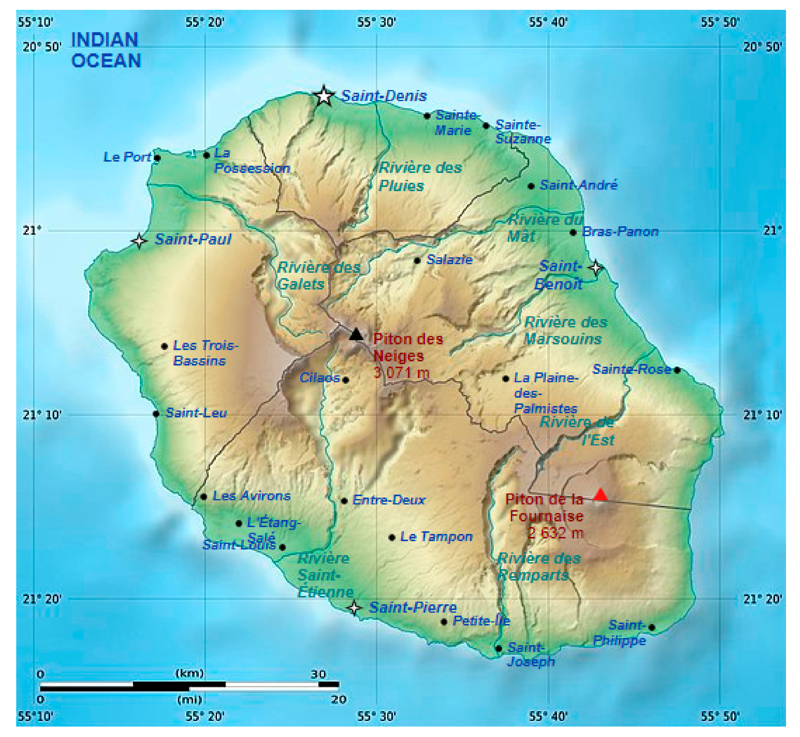
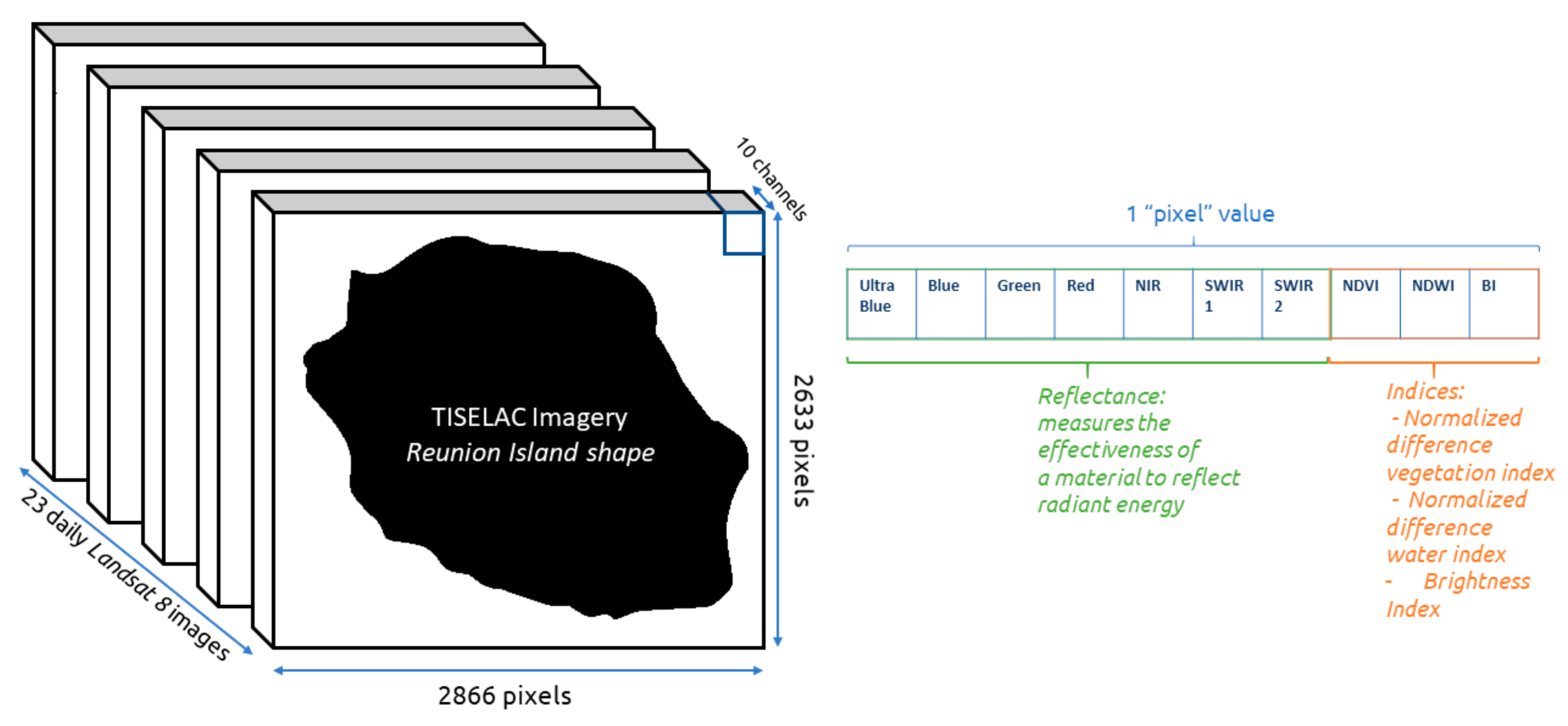
2. Materials and Study Area

The dataset (TiseLac) comprises satellite images from an annual Landsat8 time series (https://sites.google.com/site/dinoienco/tiselac-time-series-land-cover-classification-challenge, accessed on 17 September 2022) of 23 high-resolution images of dimensions of 2866 × 2633 pixels of the Reunion Island at level 2A processing recorded in 2014. A dataset is made up of pixels: 230 columns, 10 features, and 23 dates. Amongst the training and test datasets, 99,687 time series at a 30 m spatial resolution are presented by the pixels from the 23 satellite images. The training set contains 81,714 instances, whereas the testing set contains 17,973 pixels taken from the 23 landsat8 images. Each pixel has ten features at each timestamp: seven surface reflectances, one for each independent multi-spectral band (OLI): ultra-blue, blue, green, red, near-infrared (NIR), short-wave infrared (SWIR1), and SWIR2 and 3 indices computed from these surface reflectance values, normalized difference vegetation index (NDVI), normalized difference water index (NDWI), and brightness index (BI). Each sample in the time-series dataset is arranged in temporal order, with features from 1 to 10 representing the initial timestamp and features from 220 to 230 representing the final timestamp. Table 1 shows the distribution of classes in the TiSeLaC dataset. Figure 1 depicts the details of the study region. This categorization addresses three significant difficulties that might be exploited and linked to land cover data. Each sample is assigned to one of nine distinct classes. The essential perspective classes are retained, and spatial processing is used, supported by photo interpretation. The dataset was randomly sampled using pixels to create the fairest and most accurate ground truth possible. This classification aspired to accomplish two fundamental exploitable challenges associated with the land cover data for the time-series images.
  • The rich band information comprises ten features with a description of each pixel.
  • Temporal data are showcased with the 23 time-points, amongst which band features are considered. The spatial information is associated with each pixel in the form of coordinates.
Figure 1. Reunion Island showcasing all the surrounding land areas. (The arrows Piton des Neiges (southwestern) and piton de la Fournaise (eastern side) represents shield volcanoes of the reunion island in the Indian ocean).
Remotesensing 14 05232 g001
Table 1. Overview of class distributions in the training and testing datasets for the TiSeLaC dataset.
Class IDClass NameInstances TrainInstances Test
1Urban areas16,0004000
2Other built-up surfaces3236647
3Forests16,0004000
4Sparse vegetation16,0003398
5Rocks and bare soil12,9422599
6Grassland56811136
7Sugarcane crops76561531
8Other crops1600154
9Water2599519
The table shows that class proportions are equivalent between train and test splits and are a little unbalanced regarding minority classes such as other crops and water. The various land cover classes are 1. urban areas (UAs); 2. other built-up surfaces (OBAs); 3. forests (Fr); 4. sparse vegetation (SV); 5. rocks and bare soil (RBS); 6. grassland (GL); 7. sugarcane crops (SCs); 8. other crops (OCs); and 9. water (Wr). Figure 2 depicts the specifics of the dataset with the indices. The number of satellite platforms that collect remotely sensed data is constantly expanding. However, only a few labeled data are available due to the high cost in terms of money and human resources for labeling data through field campaigns or through expert knowledge. The lack of reference data, or labeled data, as well as the current availability of time series with high spatial resolutions, becomes a challenging task for assessing the validity of the proposed approaches. A fixed train and test sets are coming from the same satellite images. Therefore, they cover the same time period, and the training and testing data have the same distribution. Both vegetation classes (such as forests) and non-vegetation classes (e.g., urban areas) are included in the TiSeLaC dataset. Most land cover classes have a significant level of intra-class variability in terms of time and space. The choice of the dataset was motivated due to the following properties exhibited by various land use patterns occurring in the dataset.
The specificities of the different classes are listed below:
  • Urban Areas: cities on the Reunion Island are not as dense as those in Europe. Additionally, cities have a lot of green spaces, such as tree rows that offer shade and cooler locations. Its greenness density may influence a pixel’s associated NDVI values.
  • Other built-up surfaces: these are possibly related to greenhouses, although this is an assumption. Indeed, greenhouses are frequently built-in green spaces, which could account for more intra-class variation than in urban areas.
  • Forests: the NDVI values of the forests are stable because of the tropical climate. Thus, the time series that reflects the forests exhibits high but consistent NDVI values.
  • Sparse vegetation: pixels that do not fit into any of the other classes are grouped together. Thus, a range of profiles with intermediate NDVI values are included under this class.
  • Rocks and bare soil: this class has low NDVI values (close to or below 0). The NDVI value is predicted to vary only slightly for a given pixel.
  • Grassland: this class assembles grasslands that were mowed and grazed. The regrowth rate may vary depending on irrigation, resulting in various time series profiles.
  • Sugarcane crops: since the NDVI values decrease following harvest, this time series has the most easily distinguishable characteristics. On Reunion Island, sugarcane fields occupy approximately 60% of the farmed land, and their harvesting season lasts for approximately a month.
  • Other crops: orchards and a variety of crops, such as (pineapple and bananas), make up this class (e.g., lychees and mangos). Due to the variety of crops, this class has considerable intra-class variability.
  • Water: the considerable intra-class variability in this class can be attributed to the water’s turbidity. Water clarity is measured by its turbidity, which can affect NDVI results.

3. Models Implemented

Our fundamental premise is that selecting the exemplary model architecture is critical for improving LCC performance.
Although most of the architectures implemented are well-developed techniques in remote sensing applications, we are the first to combine this set of models in the remote sensing community to experiment with and combine them for large-scale time series analysis of land cover data. Traditionally, algorithms such as SVM and RF have been used. However, some problems faced by these algorithms are: they are oblivious to the temporal dimension, insensitive to image-order, and little inductive bias for images. Some of the traditional solutions offered to solve these problems are:
  • Pre-calculating temporal features (has little effect and requires low-level feature engineering);
  • Using the nearest neighbor algorithm with temporal similarity features (computationally expensive).
With the rising popularity of neural networks, convolutional neural networks (CNNs) came to be used for the task. Generally, 2D convolutions were applied across the spatial dimension, 1D convolutions across spectral dimension, and 3D convolutions across spatial and spectral dimensions (but no temporal dimension). Additionally, 3D-CNNs were also used in videos, with 2D convolutions in the spatial dimension and 1D convolutions in the temporal dimension. In remote-sensing tasks, 1D convolution in temporal dimension or 3D convolution in temporal and spatial dimensions are known to perform much better than machine learning algorithms. Recurrent neural networks (RNNs) such as LSTMs, GRUs, and bidirectional RNNs have also been used for this task. Combinations of RNNs and 2D-CNNs were also used by merging representations learned by the two types of networks or by feeding a CNN model with the representation learned by an RNN model. They have been used for land cover change detection tasks between multi-spectral images. Disadvantages of using RNNs are the vanishing gradients problem and long training time. The authors in [20] suggested using temporal CNNs for SITS classification for improved accuracy and a shortened training time. It presents an experimental study of temporal CNNs in order to give general guidelines about how they might be used and parameterized.
In this article, we performed the LCC of SITS data. We focus on deep neural network architectures that account for spatial, temporal, and spatiotemporal information: the devised models are gated recurrent unit (GRU); temporal convolutional neural networks (TCNN); GRU+ TCNN; and the attention model on TCNN and GRU. The proposed model is also tested in a partitioned manner with the following three possible combinations, namely univariate + multivariate (U + M), univariate + multivariate+ pixel coordinates (U + M + C), and univariate + multivariate (LSTM) + coordinates. The TiSeLac dataset was trained using the following models:

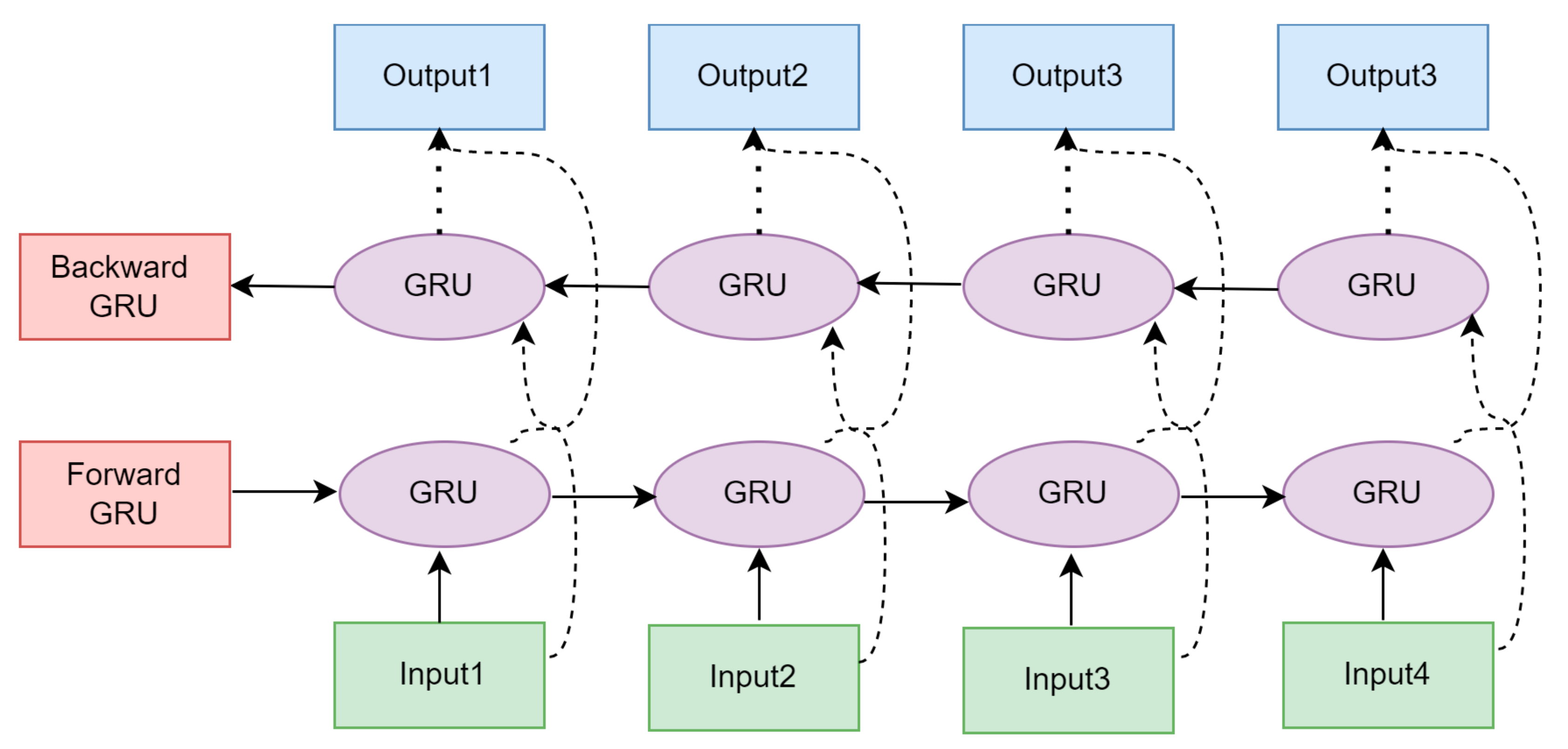
3.1. Gated Recurrent Unit

Gated recurrent unit traditional recurrent neural networks (RNN) can only cope with forward-to-backward sequences. Because they are unable to learn future information, they may lose it. As a result, the bidirectional recurrent neural network (Bi-RNN), which incorporates an RNN to deal with future input, was introduced by [44]. Bi-RNN is built by dividing a regular RNN into two directions, one moving clockwise and the other with reverse time. The same output layer is linked to both RNNs, as shown in Figure 3. This architecture can provide detailed background data for the output layer intake sequence. The historical input data must penetrate both a forward and a reverse GRU, gathering the contextual data of a complete time series to simulate sequence-level LCC analysis using Bi-GRU.

3.2. Temporal CNN

The temporal CNN belongs to the category of RNNs, which aims to focus on the temporal dimension of the time series data with the consideration of the spatial data by combining 1D fully convolutional networks and causal convolutions [45]. In this model, 1D convolutions are applied across the temporal dimension. Each dataset sample is reshaped to (the number of channels x number of days). A width filter equal to the number of channels moves across the dimension of days. The land cover analysis for the SITS is performed by explicitly managing the data flow through time. This model gives far better accuracy than the previous model, with a much shorter training time.

3.3. GRU + Temporal CNN

In this model, both GRU and temporal CNNs are used separately on the dataset. The outputs of these are concatenated together and this concatenated tensor is passed through a few fully connected layers, terminating with a nine-way SoftMax. The accuracy of this model is slightly higher than the temporal CNN model, however, the training time per epoch is higher. Increasing the number of GRUs that are stacked together in this model does not help in improving the accuracy but does increase the training time. Hence, it should be avoided.

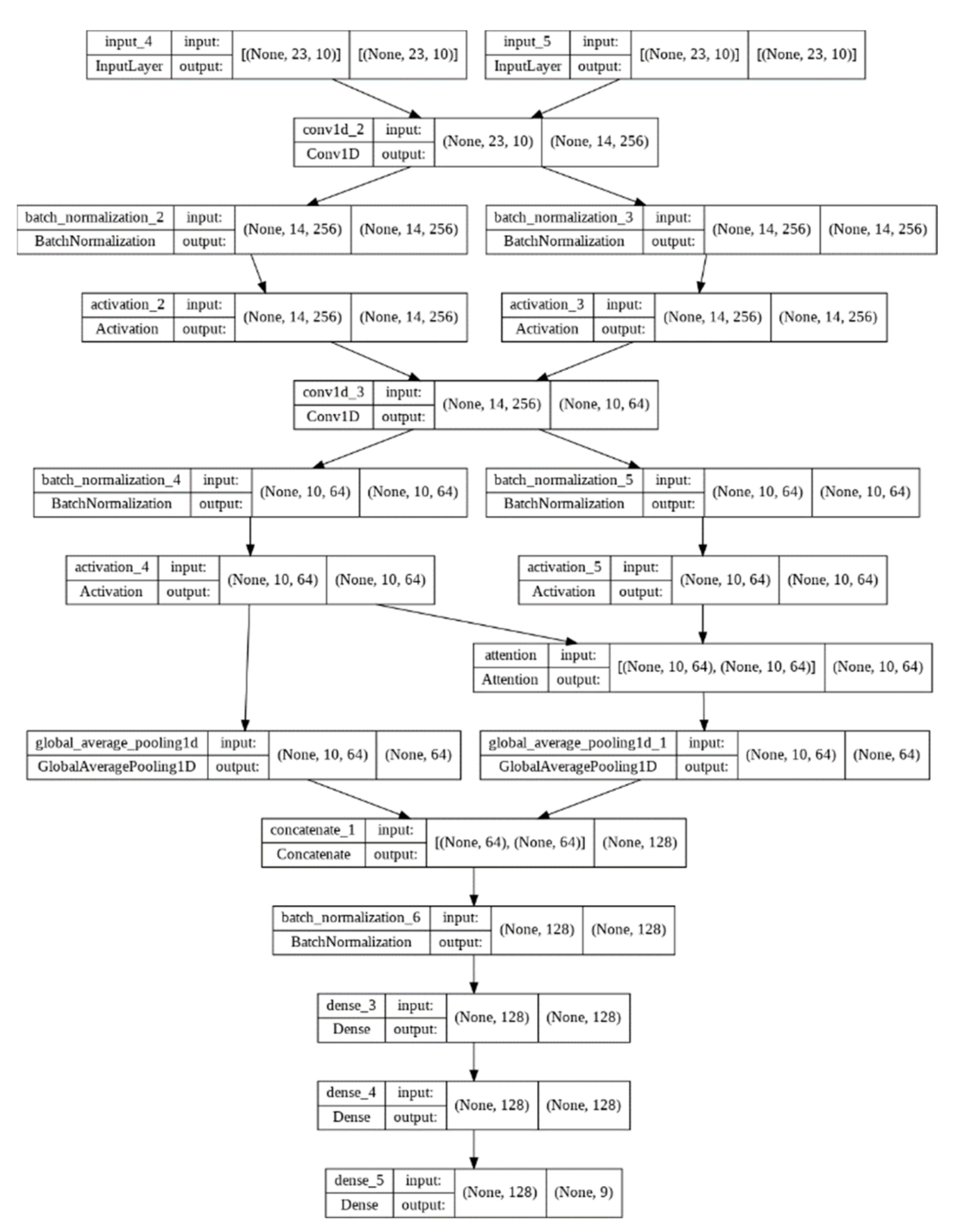
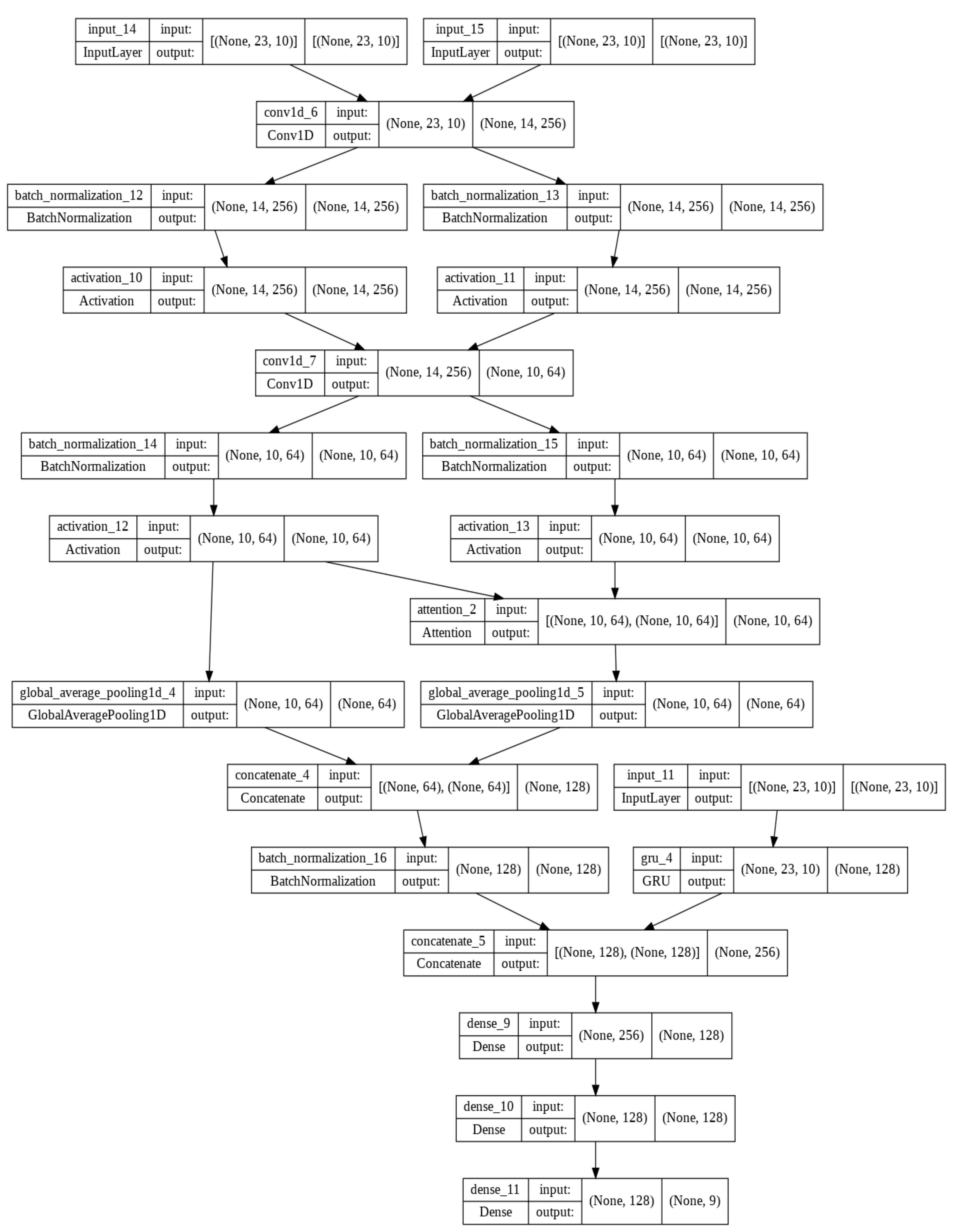
3.4. Attention on Temporal CNN and GRU

Attention models are neural network input processing methods that let the network concentrate on individual components of a complicated input one at a time until the entire dataset is classified. The idea is to divide challenging activities into manageable attentional sequentially processed chunks. A function called attention is used to translate a query to an output from an “s set” of key-value pairs. In this scenario, the end output, the fundamental values, and the query are all vectors. The weights assigned to each value are then stated by the query’s compatibility function with the associated key value. The result is then computed as a weighted sum of the values. The intuition behind using attention for our task is that the time series data of some days may be more crucial than others to predict land cover, and attention enables us to capture this [46]. Figure 4 provides the architecture of temporal CNN with an attention mechanism. Attention was applied to the temporal CNN model and the GRU + temporal CNN model.

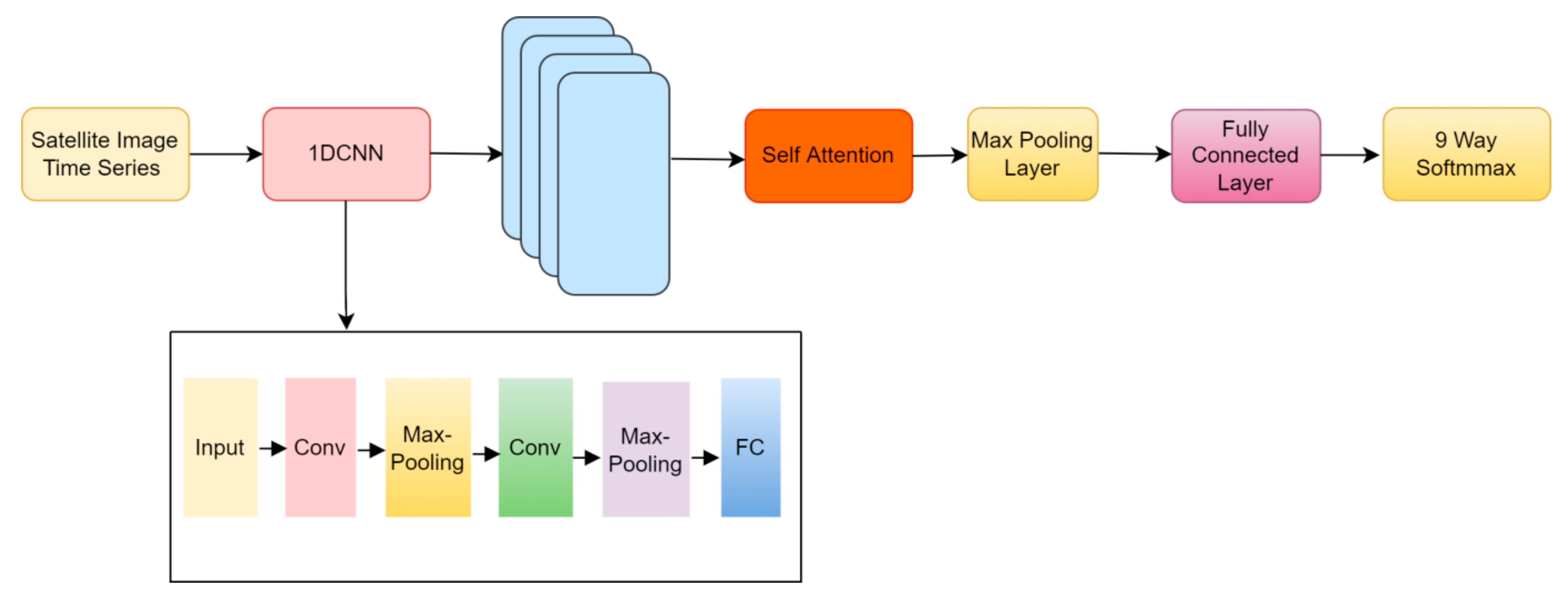
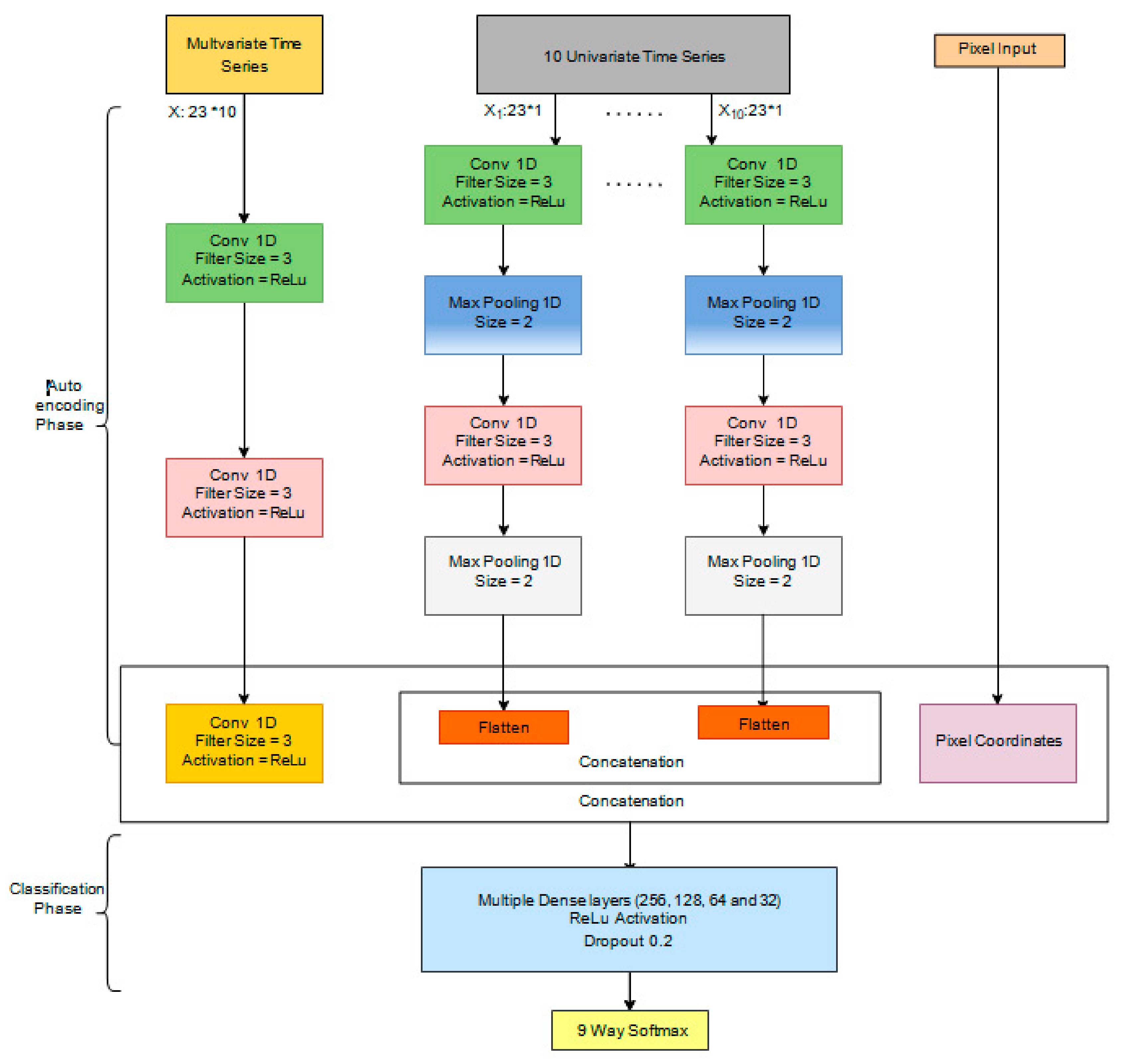
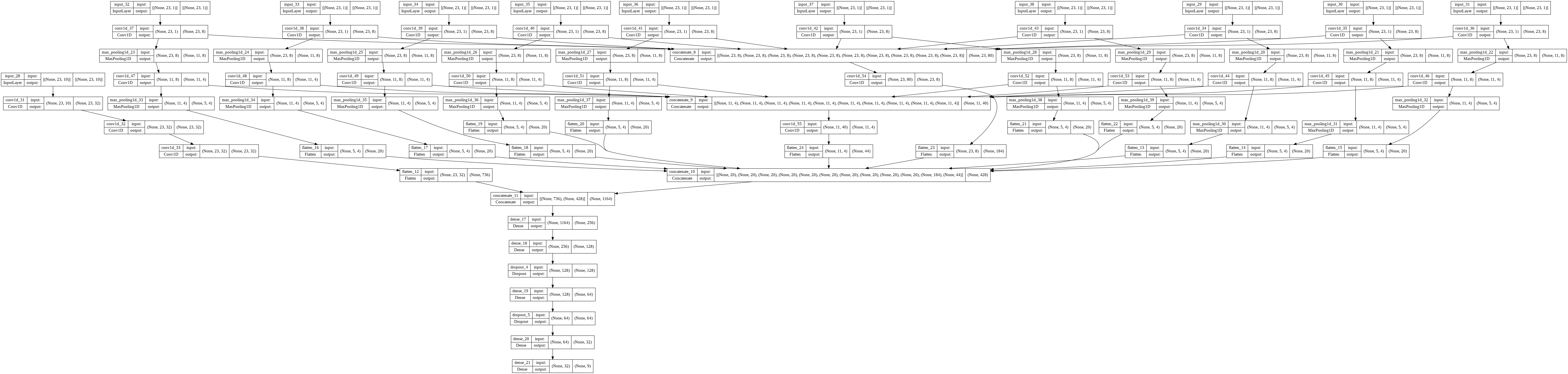
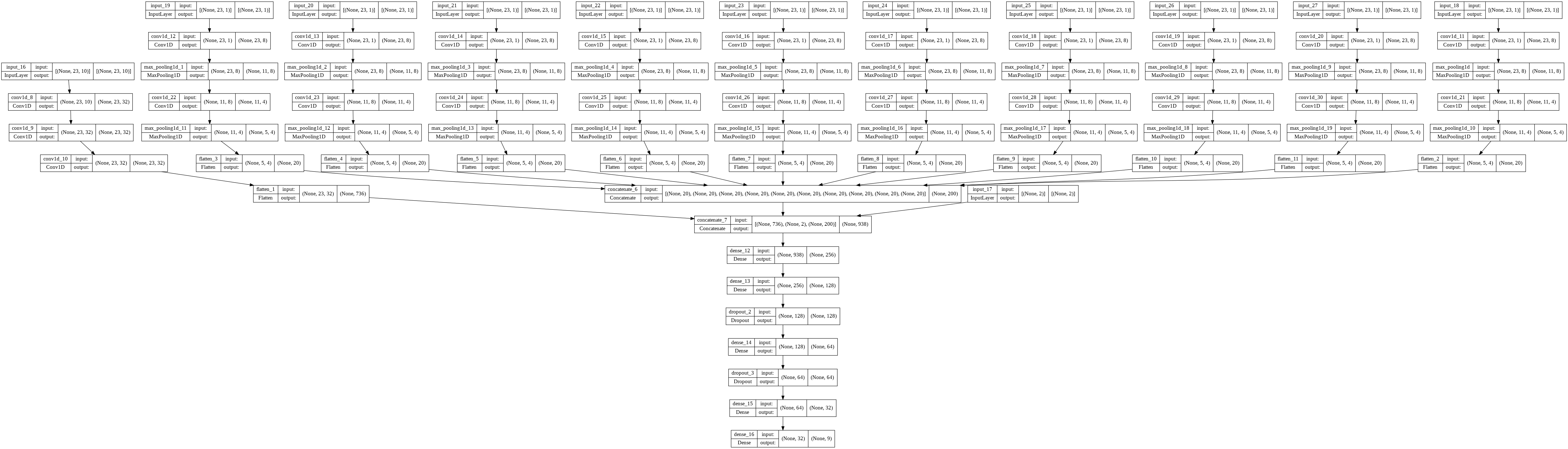
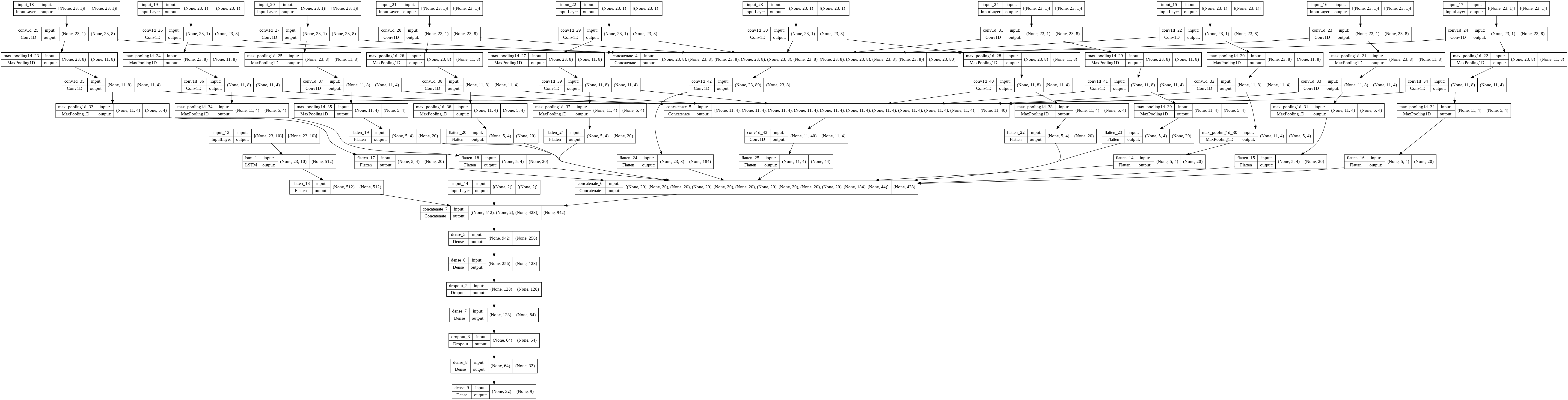
3.5. Proposed Framework

The architecture proposed in Figure 5 integrates three different models: the multivariate model on the left, ten univariate models in the center, and a model for aggregation to position the information on the right. The description is as given below:
  • Multivariate model: uses a 1D convolution on the actual data. It consists of three convolutional layers with no presence of pooling layers in between with a filter size of 3 and a RELU activation function.
  • Univariate model: this model makes use of 10 univariate models, uses 1D convolutions individually for each feature and concatenates the results. It comprises two convolution layers, including max-pooling and flatten layers at both levels. Both layers’ outcomes are concatenated to engineer the features at different levels.
  • Pixel coordinates: this model is utilized to pass through the preprocessed and scaled pixel coordinates to the final set of fully connected layers. Then, each of these feature extraction model outputs is concatenated to be classified with the usual fully connected layers.
The concatenation of these models is performed for the task of LCC on the Tiselac dataset. The variants of the proposed framework are implemented using the univariate + multivariate + coordinates component, univariate + multivariate component, and univariate + multivariate (LSTM) + coordinates component.
Figure 5. Proposed framework of univariate + multivariate + pixel coordinates for land cover classification.
Remotesensing 14 05232 g005

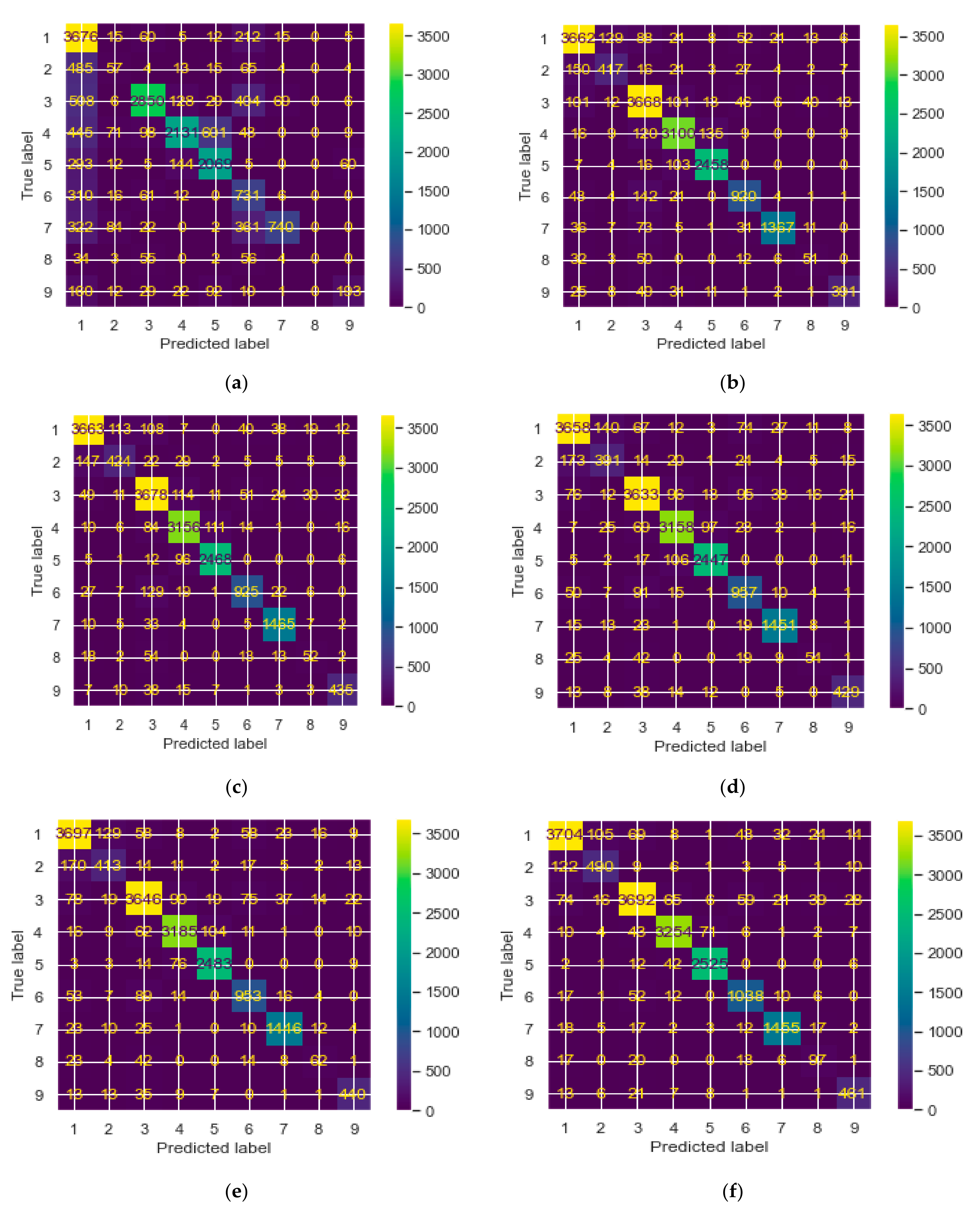
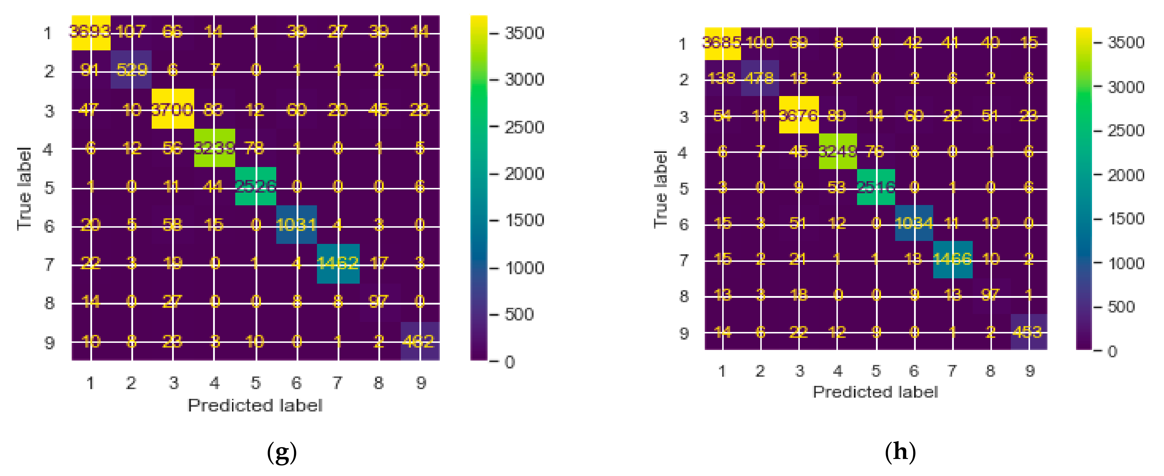
4. Experiments and Results

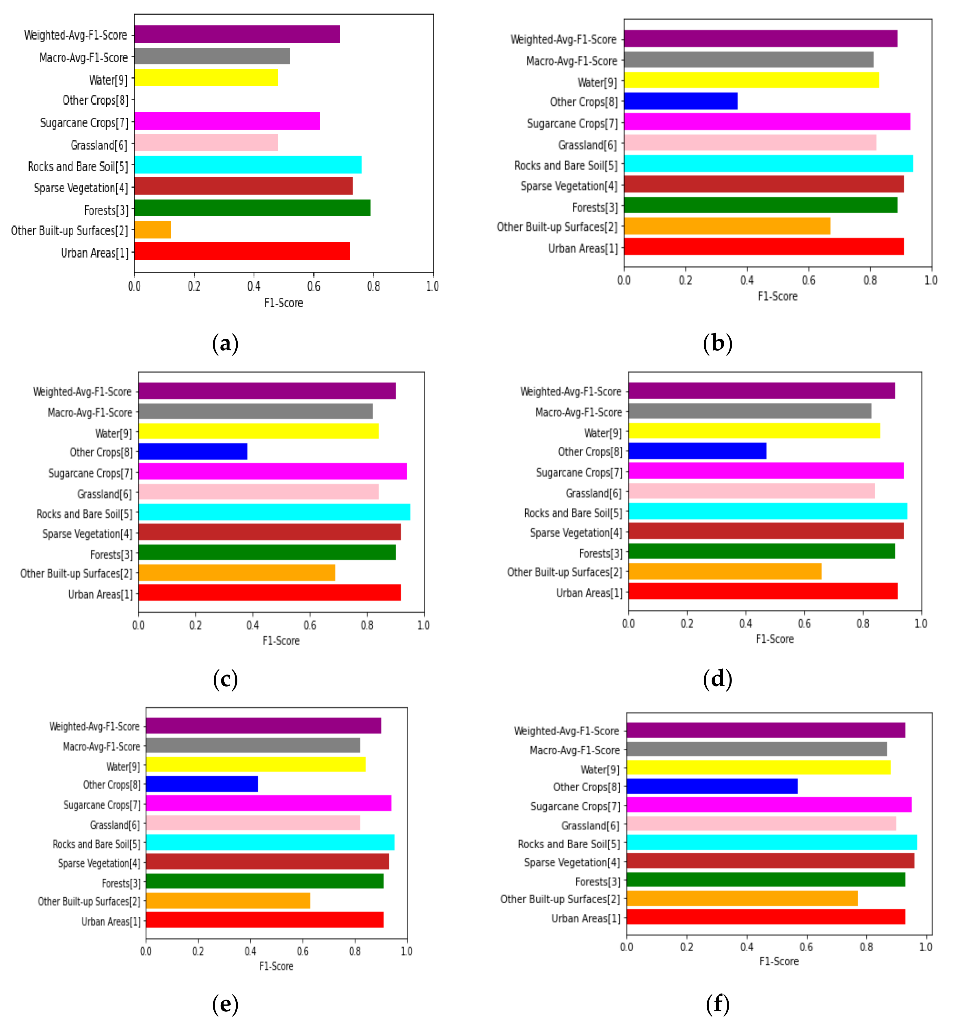
4.1. Evaluation Metrics

The performance of the various models for the land cover classification is evaluated using a test set described in Section 2. The metrics for evaluation are the accuracy, class wise F1 scores, and macro and weighted average of F1 scores. The F1 score is the mean of precision and recall, given as F1 = 2(P × R)/(P + R). The precision P = TP/(TP + FP) measures the relevancy of the results. The recall R = TP/(TP + FN) measures the return of the number of relevant results. The terms TP, FP, and FN denote the number of true positives, false positives, and false negatives, respectively, for each forecasted land cover class. The capability of each model is computed by calculating the F1 score of every class for the LCC. The macro-average is used to determine the general classification capacity of each model. The macro-average of the F1 scores is the average of all class-wise F1 scores, and it covers the class imbalance problem, providing attention to the rare essential classes. The weighted-average F1 score for the LCC is generated by computing the mean of all per-class F1 scores while considering each class’s support. The dataset’s number of actual class instances is referred to as support. The ’weight’ is effectively the fraction of each class’s support relative to the total of all support values. This section showcases the classification results using existing and proposed models. The LCC classification results are of temporal and spatiotemporal models. Table 2 and Table 3 shows the per-class accuracy, overall accuracy, per class F1 score, macro average, and weighted average F1 score for the eight deep learning models.
As we can see from Table 2, the basic models with spatial and temporal capability obtained comparable accuracy levels. The proposed architecture achieves higher accuracy levels than the spatiotemporal models, as shown in the last three columns of Table 3. The proposed framework achieves an overall accuracy of 93% with macro-average F1 scores of 87% and weighted average score of 93% with the overall support of 17,973 for the classification task. As we can see from the results, the proposed architecture has achieved similar accuracy and F1 scores, showcasing the model’s effectiveness for classifying the land cover in the time series data. The proposed framework’s precision, recall, and F1 scores are comparatively higher during the analysis process.

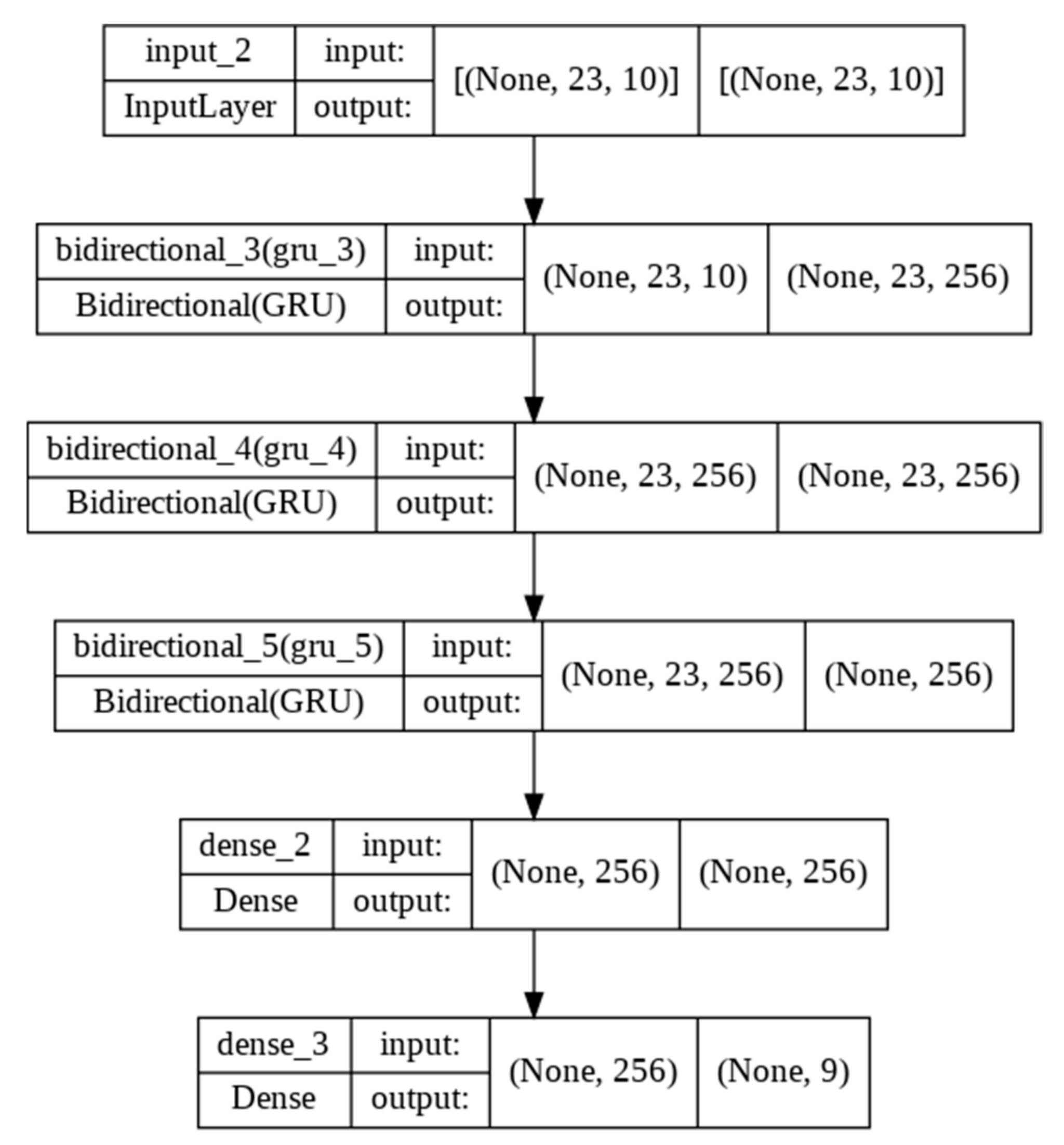
4.2. Bidirectional GRU
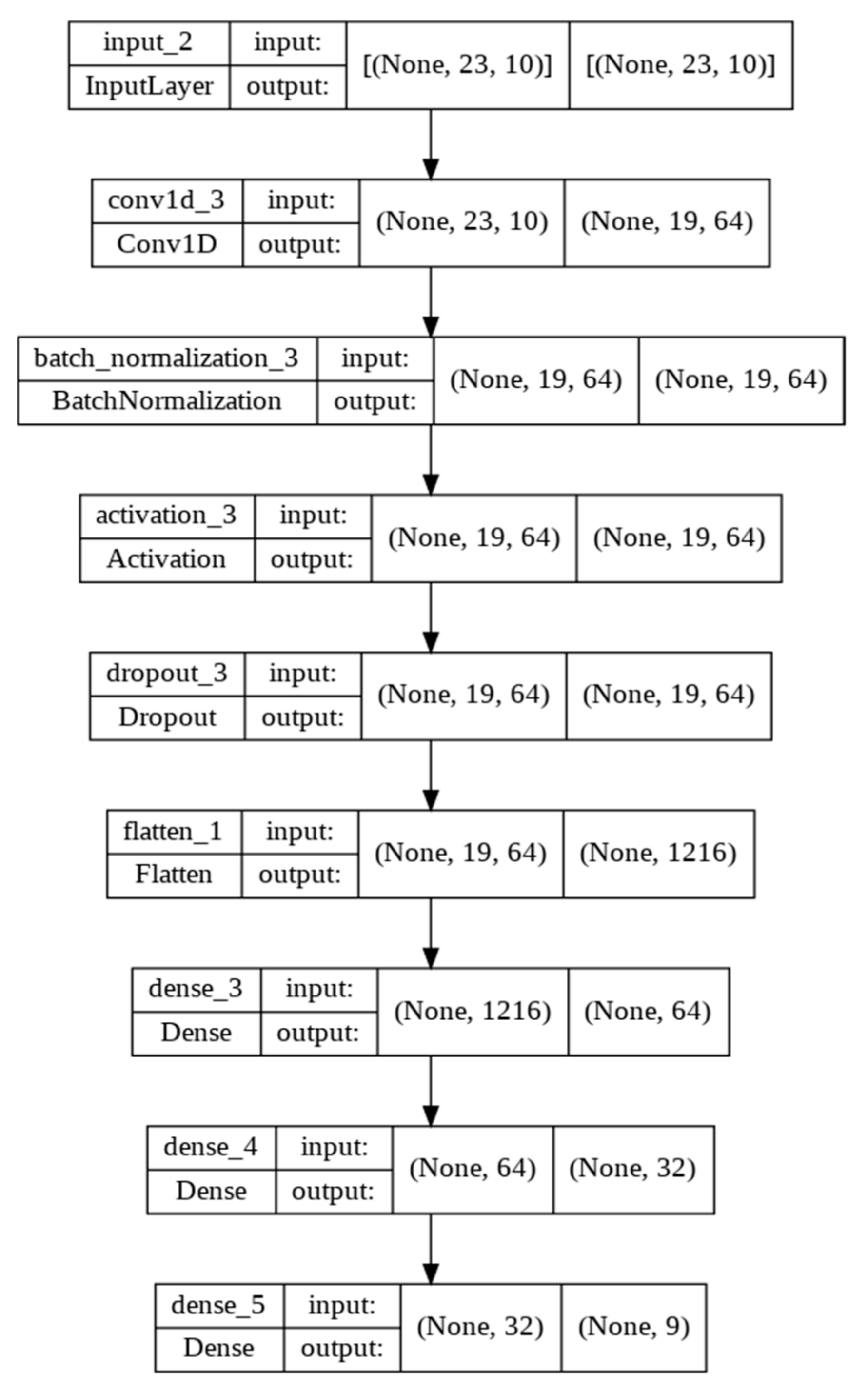
In the bidirectional GRU model, the prediction of samples is shown in the confusion matrix of Figure 6a. As can be seen in the figure, the correct prediction shows the samples showcasing a higher recall rate for the UA and Fr class and an average recall rate for the SV and RBS class, and the forecast is slightly lower for the OBS, GL, SC, OC, and Wr classes. The F1 score is also calculated as shown in Figure 7a, and it is zero for the other crops class, stating no prediction for this label. The overall accuracy for the bidirectional GRU model is 69%. The macro-average F1-score is 52% and the weighted average F1 score is 69%. As we can infer from the tables and the matrix, the land cover prediction is not so accurate, and lower on the recall rate for each class showing average performance.

4.3. Temporal CNN

The temporal CNN model uses 1D convolutions, and the prediction of samples is shown in the confusion matrix of Figure 6b. The correct prediction, as seen in Figure, shows that the samples showcase a higher recall rate for UA, Fr, SV, RBS, GL, SC, and Wr, and the average recall rate for OBS, and the prediction is slightly lower for the OC class. The F1 score is also calculated for each category, as shown in Figure 7b. The overall accuracy for the temporal CNN model is 69%. The macro-average F1 score is 81%, and the weighted average F1 score is 89%. As we can infer from the tables and the matrix, the land cover prediction is slightly higher on the recall rate for almost seven classes for the deep learning model.

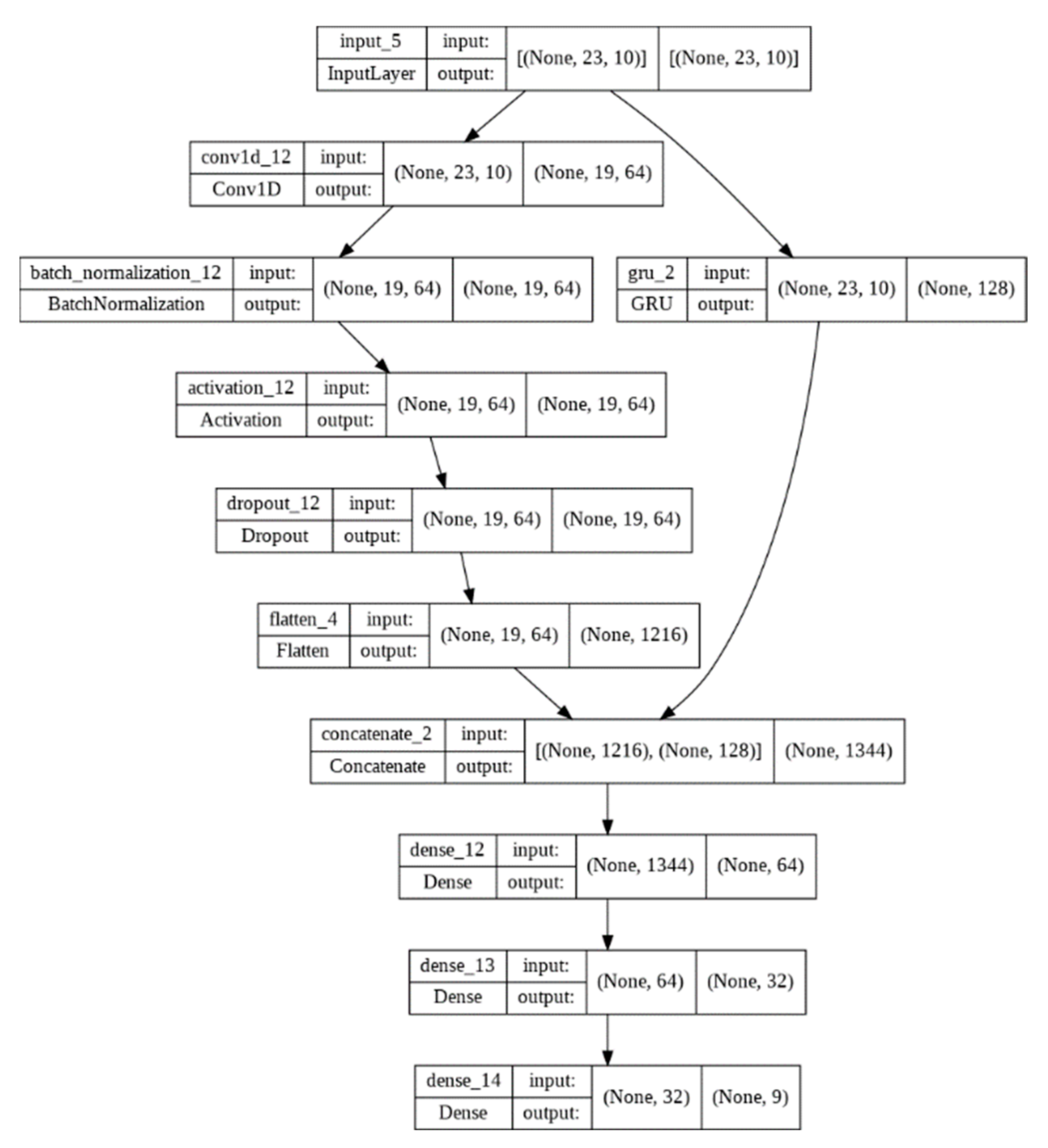
4.4. GRU + Temporal CNN

The integration of GRU and the temporal CNN model prediction of samples is shown in the confusion matrix of Figure 6c. As seen in figure, the correct prediction shows that the samples showcase a higher recall rate for UA, Fr, SV, RBS, GL, SC, and Wr average recall rate for OBS, and the forecast is slightly lower for the OC class. The F1 score is also calculated for each category, as shown in Figure 7c. The overall accuracy for the GRU + temporal CNN model is 91%. The macro-average F1-score is 82%, and the weighted average F1 score is 90%. As we can infer from the tables and the matrix, the integration of both models for the land cover prediction accuracy increased by 1% only, with the recall rate being slightly higher for almost seven classes for the deep learning model.

4.5. Attention on Temporal CNN

The attention to the temporal CNN model using self-attention and the prediction of samples are shown in the confusion matrix of Figure 6d. The correct forecast, as seen in figure, shows that the samples showcase a higher recall rate for UA, Fr, SV, RBS, GL, SC, and Wr, and an average recall rate for OBS, and the prediction is slightly lower for the OC class. The F1 score is also calculated for each category, as shown in Figure 7d. The overall accuracy for the attention on the temporal CNN model is 91%. The macro-average F1-score is 83%, and the weighted average F1 score is 91%. As we can infer from the tables and the matrix, the integration of both models for the land cover prediction accuracy has increased by 1% only, with the recall rate being slightly higher for almost seven classes for the deep learning model.

4.6. Attention on Temporal CNN + GRU

The attention to the temporal CNN with the GRU model and the prediction of samples are shown in the confusion matrix of Figure 6e. The correct prediction, as seen in figure, is that the samples showcase a higher recall rate for UA, Fr, SV, RBS, GL, SC, and Wr, average recall rate for OBS, and the prediction is slightly lower for the OC class. The F1 score is also calculated for each class, as shown in Figure 7e. The overall accuracy for the attention on the temporal CNN with the GRU model is 90%. The macro-average F1-score is 82% and the weighted average F1 score is 90%. As we can infer from the tables and the matrix, the integration of both models for the land cover prediction accuracy decreased by 1% only, with the recall rate being slightly higher for almost seven classes for the deep learning model.

4.7. Univariate + Multivariate + Coordinates

In the univariate + multivariate + coordinates model, the prediction of samples is shown in the confusion matrix of Figure 6f. As seen in the figure, the correct prediction shows that the samples showcase higher recall rates for UA, Fr, SV, RBS, GL, SC, and Wr, and average recall rates for the OBS and OC classes. The F1 score is also calculated for each category, as shown in Figure 7f. The overall accuracy for the attention on this model is 93%. The macro-average F1 score is 87%, and the weighted average F1 score is 93%. As we can infer from the tables and the matrix, the integration of the three models for the prediction of the land cover accuracy only increased by 3%, with the recall rate being higher for almost seven classes for the deep learning model.

4.8. Univariate + Multivariate

The univariate + multivariate model without the pixel coordinates performs the prediction of samples, as shown in the confusion matrix of Figure 6g. As seen in the figure, the correct prediction shows the samples showcasing higher recall rates for UA, OBS, Fr, SV, RBS, GL, SC, and Wr and slightly average recall rates for the OC class. The F1 score is also calculated for each category, as shown in Figure 7g. The overall accuracy for the attention on univariate + multivariate model is 93%. The macro-average F1 score is 87% and the weighted average F1 score is 93%. As we can infer from the tables and the matrix, the integration of the two models for the prediction of the land cover and the accuracy are almost the same as in the previous model, except for showing a higher recall rate on the OBS class and with the recall rate being higher for almost eight classes for the deep learning model.

4.9. Univariate + Multivariate (LSTM) + Coordinates

In the univariate + multivariate (LSTM) + coordinates model with the inclusion of LSTM (RNN), the prediction of samples is shown in the confusion matrix of Figure 6h. As seen in the figure, the correct prediction shows the samples showcasing higher recall rates for UA, Fr, SV, RBS, GL, SC, and Wr, with slightly average recall rates for the OBS and OC classes. The F1 score is also calculated for each class, as shown in Figure 7h. The overall accuracy for the attention on the univariate + multivariate (LSTM) + coordinates model is 93%. The macro-average F1 score is 87%, and the weighted average F1 score is 93%. As we can infer from the tables and the matrix, the integration of the two models for the prediction of the land cover and the accuracy are almost the same as in the previous model, except for showing a higher recall rate on the OBS class and with the recall rate being higher for almost eight classes for the deep learning model.

4.10. Qualitative Comparisons

As observed in Table 1 and Table 2, the accuracies of various models are being calculated to validate each deep learning model. As the number of training epochs increases, the accuracy of the validation set continues to improve and eventually tends to converge. The accuracy of the GRU model may exhibit high-level properties for extracting features from sequential data. Nonetheless, in this case, it is very low due to the longer training time and the occurrence of the vanishing gradient problem. For the temporal CNN model, as the convolutions are causal (i.e., no leakage of information) from the future to the past, they could not achieve higher accuracy for the LCC task even if they consisted of a longer memory. Due to the greater memory requirement during evaluation leading to effective data storage, the temporal CNN may perform low due to not having a larger receptive field. For the GRU + temporal CNN, increasing the number of GRUs that are stacked together does not help improve the accuracy but does increase the training time, achieving a lower accuracy for this model. The intuition behind using attention for our task is that the time series data of some days may be more critical than others to predict land cover, and attention enables us to capture this. In the case of the attention mechanisms on the temporal CNN and GRU, however, it uses an effective convolutional structure of TCNN for the extraction of temporal dependencies. The accuracy of this model is approximately higher but not above the proposed framework due to the identification of essential time steps recognized by the attention mechanism. Nevertheless, it may not be relevant to the classification task and its covariates for improving the interpretability of the land cover classes. The proposed framework achieved the highest accuracy for all models providing a higher F1 score for all the land cover classes and showcasing the extraordinary features of convolutions, and pooling layers on the univariate, multivariate, and pixel coordinates data for the effective prediction and classification of the LCC task.

5. Discussion

This study aimed to evaluate the effectiveness of various spatiotemporal deep learning models for determining land cover on a broad scale in the Reunion Island. Large-scale experiments and analyses are conducted using a real dataset derived from freely available SITS data (2000–2005) and test data supplied with the dataset. Our research findings indicate that, for the study of LCC, models that can rely on spectral or temporal information (GRU) perform lower than those that consider spatial and temporal patterns in model design decisions [47]. The proposed framework achieves higher accuracy levels to demonstrate that the LCC capabilities of CNN (spatial) and LSTM (temporal) algorithms are rather limited. When analyzing the challenge of LCC at the regional level, the research demonstrates that spatial land cover patterns are more valuable for land cover characterization than temporal patterns. This might imply more significant heterogeneity in the temporal patterns that define each land cover, presumably due to regional variances in seasonality and land cover activities.
Regarding the study, goals presented the performance of several deep learning architectures were compared for exploiting the properties of SITS. The designed and implemented models for the LCC task provided a good level of accuracy, showcasing how each model can be effectively utilized for this task. As observed in Table 2, the accuracies and the F1 score have shown an average performance for the GRU, temporal CNN, and the combination of both the models, showing an accuracy of 91%. Concerning the attention models in Table 2 and Table 3 on temporal CNN and GRU, the accuracy and F1 scores are almost similar in performance, with an accuracy of 91% and 90% showcasing a higher accuracy and F1 score in comparison to the GRU and temporal CNN models. For the proposed models, as seen in Table 3 for the classification of land covers, the combination of univariate, multivariate, and pixel coordinates exhibited an excellent performance showing an accuracy of 93% for all the models implemented.
Similar studies also exploited the time series for the LCC task in various countries such as Great Britain (Southampton and Manchester) with multilayer perceptron (MLP), CNN, with iterative updating through the Markov process [47]. The extension to this work in [47] with object-based CNN and MLP was carried out for southern England (Bournemouth and Southampton) and in northwest England (Manchester) [48]. Using a combination of deep learning and multiple classifier systems such as 1D-CNN, TCNN, and LSTM, time series classification is performed for the Sutter and Kings in California, United States [49]. LCC from multi-temporal and multispectral remotely sensed imagery for the Florida Everglades ecosystem was performed using a patch-based RNN framework [50]. Ensemble CNN, including VGGNET, and NASNET, were incorporated in a fused manner for the land use classification of crop images for the Thailand region [51]. A variety of segmentation models and the proposed deep learning model called atrous spatial pyramid pooling U-Net (ASPP-U-Net) were utilized for LCC for the center-south of China [52]. Multispectral LCC using a deep belief network was carried out for the Dadukou District of Chongqing, northern Negev, and the Changping region of Beijing [53]. The assessment of deep learning techniques for land use–land cover classification in southern New Caledonia was performed using AlexNet, ResNet, Segnet, and Deeplab architectures in [54].
Our approach is fully automated, requires very little feature engineering and integrates into a single deep architecture with both CNNs and fully connected layers to leverage the spatiotemporal nature of the data. Our method takes advantage of the data’s spatiotemporal characteristics by combining CNNs and pixel coordinates into a single deep architecture with complete automation and a minimal need for feature engineering.
Our model exploits the spatial information of each pixel. The three main components of our architecture consist of parameters that are trained jointly. The basic building blocks are one-dimensional convolutional layers, dense layers, etc. In our approach, the time series data being sequential exploits local and sparse connections with the weight-sharing features, which convolve a vector mask along the kernel with one input dimension. Additionally, the employment of parameter-free layers such as max pooling, activations with subsampling, the regularization of training with dropout, the flattening of the layers, and efficiently concatenating the representations of the task of LCC. Our model’s first element deals with learning representations by utilizing the dependencies and independencies between single bands. The second part models time series data by concurrently learning full-convolutional layer representations for each band. The third and final one uses an MLP to learn spatial representations over the extracted neighborhood data.
Compared to other land cover classes, the performance of all models in classifying other built-up surfaces and other crops in Reunion Island is comparatively lower, implying an additional heterogeneous spatiotemporal pattern in these occurrences. The rest of the seven land cover classes, namely urban areas, forest, sparse vegetation, rocks and bare spoil, grassland, sugarcane crops, and water, outperform the average performance with higher F1 scores, and are considered as among the majority classes which are linked with more uniform spatial patterns for the study region. Concerning the classification of samples for the proposed deep learning models in comparison with the existing models, we can observe that the predictions of urban areas, forests, sparse vegetation, rocks, and bare soil for the GRU and temporal CNN models are correctly classified at an average level. As we can observe from the confusion matrix of all models, the misclassification is only observed in the GRU model. Other models including the temporal CNN and their integration with attention were averaged.
The classification performed by the proposed framework provides a higher accuracy for almost all the land cover classes, with only other built-up surfaces and other crops being classified with an average F1 score and recall rate compared to the rest of the seven categories. Overall, the proposed framework with the inclusion of LSTM outperformed the GRU, temporal CNN, and variations on these models with the integration of attention mechanisms in the tropical environment. The findings from our approach suggest that explicitly accounting for both spatial and temporal patterns in data improves the generalization performance, which becomes higher for the proposed framework which is consistent with the findings of [18], who proposed a multi-temporal deep neural network for an LULC classification task, and [47], who utilized an MLP and CNN for LULC classification. Overall, the univariate, multivariate, and pixel coordinate models produced the best results in the study area considered, driving the use of these models for determining the landcover in the tropical setting as more encouraging by decreasing the work of employing human interpreters in identifying LULC over large areas.
With the possibility of a large amount of data being available from various satellite sensors contributing toward the production of medium and high-resolution time-series data, these proposed methods can be applied for the monitoring and assessment of the environment in terms of land use–land cover utilization. Since it is completely dependent on standard deep learning approaches such as 2D CNN, LSTM, etc., there is a higher demand for architecture designs in the deep learning domain for the classification and prediction of LULC patterns for a given area. Furthermore, this study validates that large-scale LCC tasks, can be completed without the need for spatiotemporal attributes which are manually handcrafted with the knowledge of the experts from the environmental engineering field to account for spatiotemporal land cover dependencies, which generally occurs in traditional machine learning models such as RF or SVM [55,56]. The design of models may be less interpretable during the data analysis, majorly because of the absence of a causal association between the inputs and outputs., i.e., the premier identification of the most relevant and valuable variable to be utilized for the LULC classification problem. Despite its effectiveness, technical obstacles still exist in LCC tasks for remote sensing data, such as:
  • Constrained model interpretability due to the absence of a direct causal relationship between inputs and outputs, i.e., the difficulty in determining the most significant and helpful variable for the classification task.
  • High computational demands were brought on by an increase in data volume resulting from an increase in the number of features and dimensions that the models could extract during the computational stage, leading to a greater need for training time and memory.
  • High demand for reference data brought on by intraclass variability (heterogeneity) in most of the LCC datasets.
Deep learning models exhibit the requirements of efficient processing units for executing higher computations in training the model. This may allow the models to extract more features and achieve an optimized system performance with a higher training time and the efficient use of memory resources. The necessity of test data in higher demand can occur due to heterogeneous data showcasing heterogeneity. Despite these obstacles, the deep learning area continually expands and has achieved higher classification accuracy than other standard models. Rapid advances in remote sensing are expected shortly, mainly through transfer learning and self-supervised learning for large-scale LCC tasks. In the future, we want to extend our research to anticipate, validate, and monitor changes in LULC at a broader scale using meta-learning and pan-tropical time-series data [57].

6. Conclusions

In this article, utilizing the inherent properties of SITS, we investigated the feasibility of using spatiotemporal deep learning models for LCC. This research considered eight deep learning models: GRU, temporal CNN, GRU + temporal CNN, attention on temporal CNN, attention on temporal CNN + GRU, multivariate + univariate + pixel coordinate with its three variants and the inclusion of LSTM for multivariate data. The spatiotemporal and temporal models were assessed for the Reunion Island dataset. In comparison to the GRU and temporal CNN, which are only made to concentrate on temporal features, we discovered that, for the majority of land cover classes, the complementary spatiotemporal information extracted by the proposed model (univariate + multivariate + pixel coordinates) from the SITS significantly increased the accuracy of the model in the classification of the land cover classes.
Despite this, the regional heterogeneity and fluctuation in the spatiotemporal properties of the land cover class during substantial evaluations make it challenging to classify the land cover using satellite images. Clouds and shadows often dominate Reunion Island tropical regions, significantly contributing to classification difficulties during the learning process. However, the examined spatiotemporal models, exceptionally trained on regional data, could effectively identify the land cover classes. The magnitude and scope of this study make it potentially valuable for monitoring large-scale changes in land cover classes and forest areas in the context of the global assessment and future agenda for Sustainable Development Goals. We discuss the difficulties with large-scale land cover evaluations on the tropical island in this work, including the variability of land covers and defining land cover rather than merely land use.
Our proposed approach can assist a more in-depth examination of where forests are lost over time and the related land cover activities. This will enable the respective environmental monitoring agencies to mitigate efforts to be focused on a few critical proximal ecological factors to have a more significant impact. Our method may be adjusted using local or national data, employs open-source platforms and data, and might be used for national environment monitoring systems. Our approach might be improved to monitor land cover all the time to find hotspots and regional trends of land use–land cover change. Further data sources may be used, such as information on recent forest losses and satellite sources (such as synthetic aperture radar images and high-resolution data).
The visualization plots of all the models implemented for the classification of land cover are shown in Appendix A from Figure A1, Figure A2, Figure A3, Figure A4, Figure A5, Figure A6, Figure A7 and Figure A8 for the reference.

Author Contributions

This paper’s investigation, resources, data curation, writing—original draft preparation, writing—review and editing, and visualization were conducted by N.N.N. and K.C. This paper’s conceptualization and software were conducted by V.M.S. and P.P. The validation, formal analysis, methodology, supervision, project administration, and funding acquisition of the version to be published were conducted by A.S. All authors have read and agreed to the published version of the manuscript.

Funding

This research received no external funding.

Institutional Review Board Statement

Not applicable.

Informed Consent Statement

Not applicable.

Data Availability Statement

Not applicable.

Conflicts of Interest

The authors declare no conflict of interest.

Appendix A

Figure A1. Bidirectional gated recurrent unit.
Remotesensing 14 05232 g0a1
Figure A2. Temporal CNN.
Remotesensing 14 05232 g0a2
Figure A3. GRU + temporal CNN.
Remotesensing 14 05232 g0a3
Figure A4. Attention on temporal CNN.
Remotesensing 14 05232 g0a4
Figure A5. Attention on GRU + temporal CNN.
Remotesensing 14 05232 g0a5
Figure A6. Univariate + multivariate.
Remotesensing 14 05232 g0a6
Figure A7. Univariate + multivariate + coordinates.
Remotesensing 14 05232 g0a7
Figure A8. Univariate + multivariate (LSTM) + coordinates.
Remotesensing 14 05232 g0a8

References

  1. Chen, L.; Jin, Z.; Michishita, R.; Cai, J.; Yue, T.; Chen, B.; Xu, B. Dynamic monitoring of wetland cover changes using time-series remote sensing imagery. Ecol. Inform. 2014, 24, 17–26. [Google Scholar] [CrossRef]
  2. Kussul, N.; Lavreniuk, M.; Skakun, S.; Shelestov, A. Deep learning classification of land cover and crop types using remote sensing data. IEEE Geosci. Remote Sens. Lett. 2017, 14, 778–782. [Google Scholar] [CrossRef]
  3. Olen, S.; Bookhagen, B. Mapping damage-affected areas after natural hazard events using sentinel-1 coherence time series. Remote Sens. 2018, 10, 1272. [Google Scholar] [CrossRef] [Green Version]
  4. Inglada, J.; Vincent, A.; Arias, M.; Tardy, B.; Morin, D.; Rodes, I. Operational high resolution land cover map production at the country scale using satellite image time series. Remote Sens. 2017, 9, 95. [Google Scholar] [CrossRef] [Green Version]
  5. Wulder, M.A.; White, J.C.; Goward, S.N.; Masek, J.G.; Irons, J.R.; Herold, M.; Cohen, W.B.; Loveland, T.R.; Woodcock, C.E. Landsat continuity: Issues and opportunities for land cover monitoring. Remote Sens. Environ. 2008, 112, 955–969. [Google Scholar] [CrossRef]
  6. Khiali, L.; Ienco, D.; Teisseire, M. Object-oriented satellite image time series analysis using a graph-based representation. Ecol. Inform. 2018, 43, 52–64. [Google Scholar] [CrossRef] [Green Version]
  7. Hay, G.J.; Castilla, G. Geographic Object-Based Image Analysis (GEOBIA): A new name for a new discipline. In Object-Based Image Analysis; Springer: Berlin/Heidelberg, Germany, 2008; pp. 75–89. [Google Scholar]
  8. Nguyen, L.H.; Joshi, D.R.; Clay, D.E.; Henebry, G.M. Characterizing land cover/land use from multiple years of Landsat andMODIS time series: A novel approach using land surface phenology modeling and random forest classifier. Remote Sens. Environ. 2020, 238, 111017. [Google Scholar] [CrossRef]
  9. Singh, B.; Venkatramanan, V.; Deshmukh, B. Monitoring of land use land cover dynamics and prediction of urban growth using Land Change Modeler in Delhi and its environs, India. Environ. Sci. Pollut. Res. 2022, 29, 71534–71554. [Google Scholar] [CrossRef]
  10. Stürck, J.; Schulp, C.J.; Verburg, P.H. Spatio-temporal dynamics of regulating ecosystem services in Europe–the role of past and future land use change. Appl. Geogr. 2015, 63, 121–135. [Google Scholar] [CrossRef]
  11. Nguyen, H.; Pham, T.; Doan, M.; Tran, P. Land Use/Land Cover Change Prediction Using Multi-Temporal Satellite Imagery and Multi-Layer Perceptron Markov Model. Int. Arch. Photogramm. Remote Sens. Spat. Inf. Sci. 2020, 2020, 99–105. [Google Scholar] [CrossRef]
  12. Ienco, D.; Gaetano, R.; Dupaquier, C.; Maurel, P. Land cover classification via multitemporal spatial data by deep recurrent neural networks. IEEE Geosci. Remote Sens. Lett. 2017, 14, 1685–1689. [Google Scholar] [CrossRef] [Green Version]
  13. Xie, S.; Liu, L.; Zhang, X.; Chen, X. Annual land-cover mapping based on multi-temporal cloud-contaminated landsat images. Int. J. Remote Sens. 2019, 40, 3855–3877. [Google Scholar] [CrossRef]
  14. Abade, N.A.; de Carvalho Júnior, O.A.; Guimarães, R.F.; De Oliveira, S.N. Comparative analysis of MODIS time-series classification using support vector machines and methods based upon distance and similarity measures in the Brazilian Cerrado-Caatinga boundary. Remote Sens. 2015, 7, 12160–12191. [Google Scholar] [CrossRef] [Green Version]
  15. Hakkenberg, C.; Peet, R.; Urban, D.; Song, C. Modeling plant composition as community continua in a forest landscape with LiDAR and hyperspectral remote sensing. Ecol. Appl. 2018, 28, 177–190. [Google Scholar] [CrossRef]
  16. Belgiu, M.; Csillik, O. Sentinel-2 cropland mapping using pixel-based and object-based time-weighted dynamic time warping analysis. Remote Sens. Environ. 2018, 204, 509–523. [Google Scholar] [CrossRef]
  17. Shao, Y.; Lunetta, R.S.; Wheeler, B.; Iiames, J.S.; Campbell, J.B. An evaluation of time-series smoothing algorithms for land-cover classifications using MODIS-NDVI multi-temporal data. Remote Sens. Environ. 2016, 174, 258–265. [Google Scholar] [CrossRef]
  18. Zhong, L.; Hu, L.; Zhou, H. Deep learning based multi-temporal crop classification. Remote Sens. Environ. 2019, 221, 430–443. [Google Scholar] [CrossRef]
  19. Diek, S.; Fornallaz, F.; Schaepman, M.E.; De Jong, R. Barest pixel composite for agricultural areas using landsat time series. Remote Sens. 2017, 9, 1245. [Google Scholar] [CrossRef] [Green Version]
  20. Pelletier, C.; Webb, G.I.; Petitjean, F. Temporal convolutional neural network for the classification of satellite image time series. Remote Sens. 2019, 11, 523. [Google Scholar] [CrossRef] [Green Version]
  21. Wubie, M.A.; Assen, M.; Nicolau, M.D. Patterns, causes and consequences of land use/cover dynamics in the Gumara watershedof lake Tana basin, Northwestern Ethiopia. Environ. Syst. Res. 2016, 5, 8. [Google Scholar] [CrossRef]
  22. Ojima, D.; Galvin, K.; Turner, B. The global impact of land-use change. BioScience 1994, 44, 300–304. [Google Scholar] [CrossRef]
  23. Bartholome, E.; Belward, A.S. GLC2000: A new approach to global land cover mapping from Earth observation data. Int. J. Remote Sens. 2005, 26, 1959–1977. [Google Scholar] [CrossRef]
  24. Gong, P.; Wang, J.; Yu, L.; Zhao, Y.; Zhao, Y.; Liang, L.; Niu, Z.; Huang, X.; Fu, H.; Liu, S.; et al. Finer resolution observation andmonitoring of global land cover: First mapping results with Landsat TM and ETM+ data. Int. J. Remote Sens. 2013, 34, 2607–2654. [Google Scholar] [CrossRef] [Green Version]
  25. Abdi, A.M. Land cover and land use classification performance of machine learning algorithms in a boreal landscape using Sentinel-2 data. GIScience Remote Sens. 2020, 57, 1–20. [Google Scholar] [CrossRef] [Green Version]
  26. Zhai, Y.; Qu, Z.; Hao, L. Land cover classification using integrated spectral, temporal, and spatial features derived from remotely sensed images. Remote Sens. 2018, 10, 383. [Google Scholar] [CrossRef] [Green Version]
  27. Lacerda Silva, A.; Salas Alves, D.; Pinheiro Ferreira, M. Landsat-Based land use change assessment in the Brazilian Atlantic forest: Forest transition and sugarcane expansion. Remote Sens. 2018, 10, 996. [Google Scholar] [CrossRef] [Green Version]
  28. Arévalo, P.; Olofsson, P.; Woodcock, C.E. Continuous monitoring of land change activities and post-disturbance dynamics from Landsat time series: A test methodology for REDD+ reporting. Remote Sens. Environ. 2020, 238, 111051. [Google Scholar] [CrossRef]
  29. Comber, A.; Balzter, H.; Cole, B.; Fisher, P.; Johnson, S.C.; Ogutu, B. Methods to quantify regional differences in land cover change. Remote Sens. 2016, 8, 176. [Google Scholar] [CrossRef] [Green Version]
  30. Marmanis, D.; Datcu, M.; Esch, T.; Stilla, U. Deep learning earth observation classification using ImageNet pretrained networks. IEEE Geosci. Remote Sens. Lett. 2015, 13, 105–109. [Google Scholar] [CrossRef] [Green Version]
  31. Tracewski, L.; Bastin, L.; Fonte, C.C. Repurposing a deep learning network to filter and classify volunteered photographs for land cover and land use characterization. Geo-Spat. Inf. Sci. 2017, 20, 252–268. [Google Scholar] [CrossRef]
  32. Ge, Y.; Zhang, X.; Atkinson, P.M.; Stein, A.; Li, L. Geoscience-aware deep learning: A new paradigm for remote sensing. Sci. Remote Sens. 2022, 5, 100047. [Google Scholar] [CrossRef]
  33. Boori, M.; Paringer, R.; Choudhary, K.; Kupriyanov, A.; Banda, R. Land cover classification and build spectral library from hyperspectral and multi-spectral satellite data: A data comparison study in Samara, Russia. In Proceedings of the IV International Conference on “Information Technology and Nanotechnology” (ITNT-2018), Samara, Russia, 24–27 April 2018; Volume 2210, pp. 390–401. [Google Scholar]
  34. Castelluccio, M.; Poggi, G.; Sansone, C.; Verdoliva, L. Land use classification in remote sensing images by convolutional neural networks. arXiv 2015, arXiv:1508.00092. [Google Scholar]
  35. Interdonato, R.; Ienco, D.; Gaetano, R.; Ose, K. DuPLO: A DUal view Point deep Learning architecture for time series classification. ISPRS J. Photogramm. Remote Sens. 2019, 149, 91–104. [Google Scholar] [CrossRef] [Green Version]
  36. Rußwurm, M.; Körner, M. Multi-temporal land cover classification with sequential recurrent encoders. ISPRS Int. J. Geo-Inf. 2018, 7, 129. [Google Scholar] [CrossRef] [Green Version]
  37. Yuan, Q.; Shen, H.; Li, T.; Li, Z.; Li, S.; Jiang, Y.; Xu, H.; Tan, W.; Yang, Q.; Wang, J.; et al. Deep learning in environmental remote sensing: Achievements and challenges. Remote Sens. Environ. 2020, 241, 111716. [Google Scholar] [CrossRef]
  38. Lyu, H.; Lu, H.; Mou, L.; Li, W.; Wright, J.; Li, X.; Li, X.; Zhu, X.X.; Wang, J.; Yu, L.; et al. Long-term annual mapping of four cities on different continents by applying a deep information learning method to landsat data. Remote Sens. 2018, 10, 471. [Google Scholar] [CrossRef] [Green Version]
  39. Ebrahim, S.A.; Poshtan, J.; Jamali, S.M.; Ebrahim, N.A. Quantitative and qualitative analysis of time-series classification using deep learning. IEEE Access 2020, 8, 90202–90215. [Google Scholar] [CrossRef]
  40. Dong, L.; Du, H.; Mao, F.; Han, N.; Li, X.; Zhou, G.; Zheng, J.; Zhang, M.; Xing, L.; Liu, T.; et al. Very high-resolution remote sensing imagery classification using a fusion of random forest and deep learning technique—Subtropical area for example. IEEE J. Sel. Top. Appl. Earth Obs. Remote Sens. 2019, 13, 113–128. [Google Scholar] [CrossRef]
  41. Liu, S.; Shi, Q. Local climate zone mapping as remote sensing scene classification using deep learning: A case study of metropolitan China. ISPRS J. Photogramm. Remote Sens. 2020, 164, 229–242. [Google Scholar] [CrossRef]
  42. Cheng, G.; Yang, C.; Yao, X.; Guo, L.; Han, J. When deep learning meets metric learning: Remote sensing image scene classification via learning discriminative CNNs. IEEE Trans. Geosci. Remote Sens. 2018, 56, 2811–2821. [Google Scholar] [CrossRef]
  43. Wang, H.; Zhao, X.; Zhang, X.; Wu, D.; Du, X. Long time series land cover classification in China from 1982 to 2015 based on Bi-LSTM deep learning. Remote Sens. 2019, 11, 1639. [Google Scholar] [CrossRef]
  44. Penghua, Z.; Dingyi, Z. Bidirectional-GRU based on attention mechanism for aspect-level sentiment analysis. In Proceedings of the 2019 11th International Conference on Machine Learning and Computing, Zhuhai, China, 22–24 February 2019; pp. 86–90. [Google Scholar]
  45. Brock, J.; Abdallah, Z.S. Investigating Temporal Convolutional Neural Networks for Satellite Image Time Series Classification. arXiv 2022, arXiv:2204.08461. [Google Scholar]
  46. Garnot, V.S.F.; Landrieu, L. Lightweight temporal self-attention for classifying satellite images time series. In International Workshop on Advanced Analytics and Learning on Temporal Data; Springer: Berlin/Heidelberg, Germany, 2020; pp. 171–181. [Google Scholar]
  47. Zhang, C.; Sargent, I.; Pan, X.; Li, H.; Gardiner, A.; Hare, J.; Atkinson, P.M. Joint Deep Learning for land cover and land use classification. Remote Sens. Environ. 2019, 221, 173–187. [Google Scholar] [CrossRef] [Green Version]
  48. Zhang, C.; Harrison, P.A.; Pan, X.; Li, H.; Sargent, I.; Atkinson, P.M. Scale sequence Joint Deep Learning for land use and land cover classification. Remote Sens. Environ. 2019, 237, 111593. [Google Scholar] [CrossRef]
  49. Dou, P.; Shen, H.; Li, Z.; Guan, X. Time series remote sensing image classification framework using combination of deep learning and multiple classifiers system. Int. J. Appl. Earth Obs. Geoinf. 2021, 103, 102477. [Google Scholar] [CrossRef]
  50. Sharma, A.; Liu, X.; Yang, X. Land cover classification from multi-temporal, multi-spectral remotely sensed imagery using patch-based recurrent neural networks. Neural Netw. 2018, 105, 346–355. [Google Scholar] [CrossRef] [Green Version]
  51. Noppitak, S.; Surinta, O. Ensemble Convolutional Neural Network Architectures for Land Use Classification in Economic Crops Aerial Images. ICIC Express Lett. 2021, 15, 531–543. [Google Scholar]
  52. Zhang, W.; Tang, P.; Zhao, L. Fast and accurate land-cover classification on medium-resolution remote-sensing images using segmentation models. Int. J. Remote Sens. 2021, 42, 3277–3301. [Google Scholar] [CrossRef]
  53. He, T.; Wang, S. Multi-spectral remote sensing land-cover classification based on deep learning methods. J. Supercomput. 2021, 77, 2829–2843. [Google Scholar] [CrossRef]
  54. Rousset, G.; Despinoy, M.; Schindler, K.; Mangeas, M. Assessment of Deep Learning Techniques for Land Use Land Cover Classification in Southern New Caledonia. Remote Sens. 2021, 13, 2257. [Google Scholar] [CrossRef]
  55. Reichstein, M.; Camps-Valls, G.; Stevens, B.; Jung, M.; Denzler, J.; Carvalhais, N. Deep learning and process understanding for data-driven Earth system science. Nature 2019, 566, 195–204. [Google Scholar] [CrossRef] [PubMed]
  56. Ma, L.; Liu, Y.; Zhang, X.; Ye, Y.; Yin, G.; Johnson, B.A. Deep learning in remote sensing applications: A meta-analysis and review. ISPRS J. Photogramm. Remote Sens. 2019, 152, 166–177. [Google Scholar] [CrossRef]
  57. Rußwurm, M.; Wang, S.; Korner, M.; Lobell, D. Meta-learning for few-shot land cover classification. In Proceedings of the IEEE/CVF Conference on Computer Vision and Pattern Recognition Workshops, Seattle, DC, USA, 14–19 June 2020; pp. 200–201. [Google Scholar]
Figure 2. Timeseries landcover dataset with 23 images with the indices.
Remotesensing 14 05232 g002
Figure 3. Bidirectional Gated Recurrent Unit.
Remotesensing 14 05232 g003
Figure 4. Attention on temporal CNN.
Remotesensing 14 05232 g004
Figure 6. Confusion matrix depicting the correctly and falsely predicted LCC for Reunion Island for all the deep learning models: (a) bidirectional GRU; (b) temporal CNN; (c) GRU + temporal CNN; (d) attention on temporal CNN; (e) attention on temporal CNN + GRU; (f) univariate + multivariate + coordinates; (g) univariate + multivariate; and (h) univariate + multivariate (LSTM) + coordinates.
Remotesensing 14 05232 g006aRemotesensing 14 05232 g006b
Figure 7. F1 scores of land cover classification for the time series dataset using the deep learning model: (a) bidirectional GRU; (b) temporal CNN; (c) GRU + temporal CNN; (d) attention on temporal CNN; (e) attention on temporal CNN + GRU; (f) univariate + multivariate + coordinates; (g) univariate + multivariate; (h) univariate + multivariate (LSTM) + coordinates.
Remotesensing 14 05232 g007aRemotesensing 14 05232 g007b
Table 2. Precision, recall, and F1 score values for the GRU, temporal CNN and attention models on temporal CNN.
GRUTemporal
CNN
GRU + Temporal CNNAttention on Temporal CNN
Class IDPRF1SPRF1SPRF1SPRF1S
1 (UA)0.590.920.7240000.900.920.9140000.930.920.9240000.910.920.924000
2 (OBS)0.210.090.126470.700.640.676470.730.660.696470.680.640.66647
3 (Fr)0.900.710.7940000.870.920.8940000.880.920.9040000.910.910.914000
4 (SV)0.870.630.7333980.910.910.9133980.920.930.9233980.940.940.943398
5 (RBS)0.730.800.7625880.930.950.9425880.950.950.9525880.950.960.952588
6 (GL)0.390.640.4811360.840.810.8211360.880.810.8411360.840.840.841136
7 (SC)0.880.480.6215310.970.890.9315310.930.960.9415310.940.940.941531
8 (OC)0.000.000.001540.430.330.371540.430.340.381540.560.400.47154
9 (Wr)0.700.370.485190.920.750.835190.850.840.845190.870.850.86519
Accuracy 0.6917,973 0.8917,973 0.9117,973 0.9117,973
Macro avg0.580.520.5217,9730.830.790.8117,9730.830.810.8217,9730.840.820.8317,973
Weighted avg0.730.690.6917,9730.890.890.8917,9730.900.910.9017,9730.910.910.9117,973
Table 3. Precision, recall and F1 score values for the Attn. On temporal CNN and the univariate + multivariate + pixel coordinates.
Attention on Temporal CNN + GRUUnivariate + Multivariate+ CoordinatesUnivariate + MultivariateUnivariate + Multivariate (LSTM) + Coordinates
Class IDPRF1SPRF1SPRF1SPRF1S
1 (UA)0.910.910.9140000.930.930.9340000.950.920.9340000.930.920.934000
2 (OBS)0.650.600.636470.780.760.776470.780.820.806470.780.740.76647
3 (Fr)0.910.910.9140000.940.920.9340000.930.930.9340000.940.920.934000
4 (SV)0.920.930.9333980.960.960.9633980.950.950.9533980.950.960.953398
5 (RBS)0.950.950.9525880.970.980.9725880.960.980.9725880.960.970.972588
6 (GL)0.790.840.8211360.880.910.9011360.900.910.9011360.890.910.901136
7 (SC)0.940.950.9415310.950.950.9515310.960.950.9615310.940.960.951531
8 (OC)0.550.350.431540.520.630.571540.470.630.541540.460.630.53154
9 (Wr)0.850.830.845190.870.890.885190.880.890.895190.880.870.88519
Accuracy 0.9017,973 0.9317,973 0.9317,973 0.9317,973
Macro avg0.830.810.8217,9730.870.880.8717,9730.870.890.8717,9730.860.880.8717,973
Weighted avg0.900.900.9017,9730.930.930.9317,9730.930.930.9317,9730.930.930.9317,973
Publisher’s Note: MDPI stays neutral with regard to jurisdictional claims in published maps and institutional affiliations.

