Article

Energy-Based Adversarial Example Detection for SAR Images

1
Comprehensive Situational Awareness Group of IntelliSense Lab, National University of Defense Technology, Changsha 410073, China
2
The State Key Laboratory of Complex Electromagnetic Environmental Effects on Electronics and Information System, National University of Defense Technology, Changsha 410073, China
*
Author to whom correspondence should be addressed.
Remote Sens. 2022, 14(20), 5168; https://doi.org/10.3390/rs14205168
Submission received: 2 August 2022 / Revised: 15 September 2022 / Accepted: 3 October 2022 / Published: 15 October 2022

Abstract

:
Adversarial examples (AEs) bring increasing concern on the security of deep-learning-based synthetic aperture radar (SAR) target recognition systems. SAR AEs with perturbation constrained to the vicinity of the target have been recently in the spotlight due to the physical realization prospects. However, current adversarial detection methods generally suffer severe performance degradation against SAR AEs with region-constrained perturbation. To solve this problem, we treated SAR AEs as low-probability samples incompatible with the clean dataset. With the help of energy-based models, we captured an inherent energy gap between SAR AEs and clean samples that is robust to the changes of the perturbation region. Inspired by this discovery, we propose an energy-based adversarial detector, which requires no modification to a pretrained model. To better distinguish the clean samples and AEs, energy regularization was adopted to fine-tune the pretrained model. Experiments demonstrated that the proposed method significantly boosts the detection performance against SAR AEs with region-constrained perturbation.

Graphical Abstract

1. Introduction

Deep neural networks (DNNs) have achieved remarkable performance on synthetic aperture radar (SAR) target recognition [1]. However, adversarial attacks [2] have drawn wide public concern on the security of applicable DNN models. By adding imperceptible perturbation to a clean image, the so-called adversarial example (AE) can fool a pretrained DNN model into outputting any predictions specified by the attacker. Classic adversarial attacks [3,4,5,6] have become benchmarks to measure the robustness of neural networks. The latest research has proven that optical attacks maintain high performance when attacking DNN-based SAR image recognition models [7,8,9,10].
To meet the challenges posed by adversarial attacks, researchers have paid attention to adversarial defense. Current defenses can be decomposed to construct robust models and detect malicious inputs, i.e., adversarial detection. The first aims to improve the adversarial robustness of DNN models and correctly identify the real label of AEs [11,12,13]. The second only determines whether the test samples are AEs, such as the local intrinsic dimensionality detector (LID) [14] and Mahalanobis detector (MD) [15] in optics and the soft threshold detector (STD) [16] for remote sensing images. Adversarial detection endows DNN models with the ability to perceive the on-going adversarial attacks and has received more attention on SAR image recognition in adversarial situations.
Different from optical images, each pixel in a SAR image represents the scattering energy of electromagnetic waves reflected from the imaging area. For the physical realization, global perturbation AEs require changing the scattering characteristics of the entire imaging region, which is a rather costly task. A feasible idea is to restrict the perturbation to a certain region, and the corresponding research has recently been carried out. The current discussion focuses on generating adversarial perturbations near the target [17] and correlating the adversarial perturbation with electromagnetic signals [18] to reduce the physical realization difficulty of SAR AEs. Although no mature physical AE implementation method has been proposed yet, it is necessary to explore the security threat of region-constrained SAR AEs. From a defensive standpoint, we found that current detection methods expose performance degradation against SAR AEs with regional constraints. Designing defense methods robust to region-constrained adversarial perturbation is an ongoing challenge.
In this paper, we considered AEs to be low-probability samples that are incompatible with the clean dataset. Through energy-based models [19,20,21], we converted the probability criterion to an energy criterion, where a sample with higher energy corresponds to a stronger adversarial degree. Further, we found that there is an inherent energy gap between the distributions of clean samples and AEs on a pre-trained model, even when regional constraints are imposed on AEs. Based on this discovery, we propose the energy-based detector (ED) and the fine-tuned energy-based detector (FED) to solve the problem of detecting region-constrained SAR AEs. The contribution of this paper can be summarized as follows:
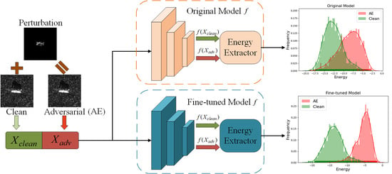
  • We designed a novel energy feature space for SAR adversarial detection, where the adversarial degree of a sample is positively related to its energy.
  • We propose an energy-based detector (ED), which requires no modification to the pretrained model. Compared with another unmodified detector, STD, the proposed method showed superior performance.
  • On the basis of ED, we propose to fine-tune the pre-trained model with a hinge energy loss item to further optimize the output energy surface. Compared with the LID and MD, the proposed fine-tuned energy-based detector (FED) was experimentally demonstrated to boost the detection performance against SAR AEs, especially for those with regional constraints.
The rest of this paper is organized as follows. In Section 2, we briefly introduce the adversarial attack and adversarial detection methods used in this paper. In Section 2.3, we explore generating SAR AEs with region-constrained perturbation and analyze the weakness of current adversarial detection methods. In Section 3, we propose our energy-based detector (ED) and fine-tuned energy-based detector (FED). In Section 4, we provide the details of the experiment. Finally, the discussion and conclusion are summarized in Section 5.

2. Preliminaries

2.1. Adversarial Attack

Adversarial attacks can be divided into targeted attacks and untargeted attacks. The prediction of a targeted AE in the model is specified by the attacker, while the prediction of an untargeted AE is any category other than its true label. In practical applications, defenders cannot know which category the upcoming attack will target. When evaluating the performance of adversarial detection, generating untargeted AEs is a common process to ensure that the defense covers each category. Since this paper is on the defensive side, we introduced adversarial attacks in an untargeted manner.
Given a sample x with a ground truth label y, an discriminative model f estimates the category of x by calculating the conditional probability of the sample x on the category y:
p ( y | x ) = e f y ( x ) i e f i ( x )
where f i ( x ) represents the i-th component of the model’s output f ( x ) . The essence of adversarial attack is to increase a model’s cross-entropy loss by adding an l-norm constrained perturbation η on a clean image x:
max η i q ( i ) · log p ( i | x + η ) s . t . η l < ε
where q ( i ) represents the ground truth probability of label i and p ( i | x + η ) represents the conditional probability of x + η on label i. For one-hot-encoded labels, Equation (2) can be simplified to:
max η log p ( y | x + η ) s . t . η l < ε
That is, the AE fools DNN classifiers by reducing the conditional probability of sample x + η on the ground truth label y.
The core of the adversarial attack is to design a suitable perturbation function η ( · ) :
  • FGSM: The fast gradient sign method (FGSM) [3] normalizes the gradients of the input with respect to the loss of model f to the smallest pixel depth as a perturbation unit:
    η F G S M ( x ) = s i g n ( x L o s s ( f ( x ) , y ) )
  • BIM: The basic iterative method (BIM) [4] optimizes the FGSM attack as an iterative version:
    η B I M ( x i + 1 ) = s i g n ( x i L o s s ( f ( x i ) , y ) )
  • DeepFool: Moosavi-Dezfooli et al. [5] added iterative perturbations until the AE crosses a linearly assumed decision boundary, and the perturbation in each iteration is calculated as
    η D e e p F o o l ( x i + 1 ) = min k f y ( x i ) f k ( x i ) y f y ( x i ) k f ( x i )
  • CW: To avoid clamping AEs between ( 0 , 1 ) in every iteration, Carlini and Wagner [6] introduced a new variable w to express the AE as 1 2 ( tanh ( w ) + 1 ) , which maps the value of the AE smoothly lying between ( 0 , 1 ) . The perturbation is expressed as:
    η C W ( x ) = 1 2 ( tanh ( w ) + 1 ) x

2.2. Adversarial Detection

Adversarial detection is essentially a binary classification problem where clean samples are treated as positives and AEs are negatives. Given a test sample x, the detector D judges its adversarial property according to a well-designed metric function M and a threshold α :
D ( x ) = adversarial , clean , M ( x ) α , M ( x ) < α .
The core of adversarial detection is to find a suitable metric function M:
  • Local intrinsic dimensionality detector (LID): Ma et al. [14] supposed that the AEs lie in the high-dimensional region of the feature manifold and, therefore, own higher local intrinsic dimensionality (LID) values compared with clean samples. Given a test sample x, the LID method randomly picks k samples in the training set and calculates the LID value of sample x as follows:
    M L I D ( x ) = ( 1 k i = 1 k log r i ( x ) r k ( x ) ) 1
    where r i ( x ) represents the featurewise Euclidean distance from sample x to its i-th nearest neighbor.
  • Mahalanobis detector (MD): Lee et al. [15] adopted the featurewise Mahalanobis distance to measure the adversarial degree of a test sample x under the assumption that clean samples obey the class conditional Gaussian distribution in the feature space, while the AEs do not. With the feature vector before the classification layer of sample x defined as V ( x ) , the metric function of the MD method is calculated as
    M M D ( x ) = V ( x ) μ k 1 V ( x ) μ k T
    where μ k is the mean feature vector of the predicted label k of x on the training set and ∑ is the feature covariance matrix.
  • Soft threshold detector (STD): Li et al. [16] found that there are differences in classification confidence between clean samples and AEs, and a lower confidence corresponds to a higher adversarial degree. Based on this finding, the authors recreated a new dataset consisting only of classification confidence and binarized labels and trained a logistic regression classifier to obtain the best confidence threshold α for each class. The metric function M of the STD method can be expressed as
    M S T D = p ( argmax f ( x ) | x )
The LID [14] and MD [15] require disassemble the model to extract the intermediate layer features, so they are usually considered as modified methods, while the STD [16] only checks the output of the model, which is an efficient unmodified method.

2.3. Problem of Detecting SAR AEs under Regional Constraint

The regional constraint of the perturbation has attracted wide attention when generating SAR AEs. Different from the physical implementation method of optical AEs, such as directly pasting adversarial patches [22,23,24], SAR images reflect the energy distribution of the scattered points formed by the electromagnetic echo of the target after being processed by the Fourier transform. Although there is yet no physical implementation method for SAR AEs, a feasible idea is to constrain the adversarial attack to a specific region to reduce the difficulty of coupling the perturbation with signals. How to defend against SAR AEs with the region constraint is a practical problem that needs to be studied urgently. In this paper, we explored the influence of four different regional constraint functions, as shown in Figure 1. Under the regional constraint, the objective function of the adversarial attack in Equation (3) will be different:
max η log p ( y | x + R η ) s . t . R η p < ε
where the constraint term R can be understood as a mask with the specified pixels of 1 and others of 0 and works by taking the Hadamard product ⊙ with the original perturbation η . The open SAR dataset MSTAR [25] and its publicly accessible segmentation annotation SARbake [26] were used as an auxiliary to design the region constraint mask R.
Taking the FGSM AE as an example, we discuss the impact of regional constraints on three classical adversarial detection methods [14,15,16], as shown in Figure 2:
  • Impact on the LID and MD: The LID and MD implement detection by examining the intermediate features of the test samples. However, as the regional constraint became tightened, the detection performance of the LID and MD showed a significant drop, with the AUROC dropping by nearly 20% in the worst case. This reveals that SAR AEs under the regional constraint not only expose smaller visual observability, but also have less difference in intermediate features from clean samples.
  • Impact on the STD: The STD method detects AEs by checking the output confidence. It can be seen that the regional constraint had relatively less impact on the output layer of the model. However, since the STD method is still based on the conditional confidence p ( y | x ) , it did not perform as well as the LID and MD, despite its computational efficiency.

3. Proposed Method

As discussed in Section 2.3, the regional constraints bring severe performance degradation to the detection methods based on intermediate features [14,15]. Although the output confidence-based method [16] is less affected by the regional constraint, it yet has limited performance due to checking the conditional probability p ( y | x ) . We hope to find a method combining both high performance and robustness to regional constraints. Different from the conditional probabilities p ( y | x ) at the output level, we believe that p ( x ) is a more reasonable choice to measure the adversarial degree of a test sample.

3.1. Interpretability of p ( x )

As shown in Equation (3), the essence of an adversarial attack is to reduce the conditional probability p ( y | x ) (confidence) of a clean sample as the true class, so that the model misjudges the corresponding AE as the wrong class. However, researchers [3,6] have shown that AEs also have high confidence (nearly 100%) in the wrong category, which results in the inability of conditional-probability-based criteria to distinguish high-confidence AEs.
Given a training set consisting of clean samples ς = ( x , y ) | x R w × h , y R , the marginal distribution p ( x ) is usually thought of as the probability of x being sampled in the training set ς . By decomposing p ( x ) into the sum of joint distributions p ( x , i ) on a k-classification model, we provide a new perspective on p ( x ) :
p ( x ) = i K p ( x , i )
The joint distribution p ( x , i ) measures the probability that sample x and label i occur at the same time or how much sample x is compatible with label i. Then, p ( x ) can be interpreted as the compatibility of x with the entire training set ς . It is well known that AEs and clean samples are visually similar x a d v x , but their predicted labels in a DNN model are quite different y a d v y . Hence, our core idea is that AEs are incompatible with the clean training set ς , indicating a low p ( x ) .

3.2. Energy-Based Detector on Pretrained Model

It is intractable to calculate p ( x ) through the sum of the joint distribution by Equation (13) on a discriminative model. Energy-based models [19,20,21] offer a new approach to this problem. LeCun et al. [19] pointed out that any probability density p ( x ) for x R can be expressed in the form of an free energy function:
p ( x ) = e E ( x ) x e E ( x ) d x = e E ( x ) Z ,
where E · is the free energy function, which maps a sample x to a scalar value. The constant Z = x e E ( x ) d x is known as the partition function, which normalizes the probability between 0 and 1. After taking the logarithm of both sides of Equation (14), we can find that log p ( x ) is linearly aligned with E ( x ) :
log p ( x ) = E ( x ) log Z
where a larger p ( x ) corresponds to a smaller E ( x ) . Hence, the problem of solving p ( x ) can be transformed into solving E ( x ) . Will et al. [20] revealed that one can reinterpret a standard discriminative classifier of p ( y | x ) as an energy-based model for the joint distribution p ( x , y ) :
p ( x , y ) = e f y ( x ) Z
where f y is the y-th component of the model’s output f ( x ) and Z is the constant partition function. According to the Bayes rule and Equation (1):
p ( x , y ) = p ( x ) · p ( y | x ) = e E ( x ) Z · e f y ( x ) i = 0 K e f i ( x )
where K is the total number of categories. By connecting Equations (16) and (17), we obtain the explicit expression for E ( x ) :
E ( x ) = log i = 0 K e f i ( x )
where the energy E ( x ) is defined by the model’s output f ( x ) . For clean samples, the logarithm of its probability p ( x ) is larger, corresponding to lower energy E ( x ) , while AEs have a smaller p ( x ) , corresponding to a higher E ( x ) .
To confirm our assumption, we visualize the energy distribution of clean samples and AEs on the test set, as shown in Figure 3. It can be observed that there is an “energy gap” between the energy distributions of clean samples and AEs even when the regional constraint is imposed on AEs. The high-energy AEs and low-energy clean samples naturally belong to two different distributions. By setting an appropriate decision threshold α , it is feasible to achieve the distinction between AEs and clean samples. Hence, we trained a logistic regression model on a small validation set ς v a l , where clean samples and the corresponding AEs are labeled as positives and negatives, respectively. Then, the energy value corresponding to a 95% true positive rate is set as the threshold α . We provide the pseudocode for training our energy detector (ED) in Algorithm 1.
Algorithm 1: Energy-based adversarial detector (ED).
Remotesensing 14 05168 i001

3.3. Energy-Based Detector on Fine-Tuned Model

Although there is an inherent energy difference between AEs and clean samples on a pretrained model, we hope to increase this “energy gap”. Hence, we define a new objective function to fine-tune a pretrained model:
min θ L C E + λ L E G
The former item L C E is the simplified cross-entropy loss derived from Equations (2) and (3), which keeps the classification accuracy of the model for clean samples:
L C E = log p ( y | x )
The latter item L E G is the energy loss, which enlarges the energy gap between the clean samples and AEs, and λ is the regularization coefficient. We used the hinge function to define the energy loss:
L E G = max ( 0 , E ( x c l e a n ) E L B ) + max ( 0 , E U B E ( x a d v ) )
where E L B and E U B are the lower bound and upper bound of energy, respectively. This loss function is designed to penalize clean samples with an energy higher than the lower bound and AEs with an energy lower than the upper bound, so that an optimized energy surface can be obtained. The mean energy of clean samples and their corresponding AEs is calculated, respectively, in the validation set ς v a l as the lower bound E L B and upper bound  E U B :
E L B = 1 N i = 0 N E ( x c l e a n ) E U B = 1 N i = 0 N E ( x a d v ) x ς v a l
We verified the effectiveness of the proposed fine-tuning method on the same test set in Section 3.2. The flowchart of the FED detector and visualization of energy distributions are shown in Figure 4. It can be observed that, after fine-tuning by Equation (19), the energy gap between AEs and clean samples are significantly enlarged. The details of acquiring our fine-tuned energy detector are provided in Algorithm 2.
Algorithm 2: Fine-tuned energy-based detector (FED).
Remotesensing 14 05168 i002

4. Results

In order to facilitate the reader’s understanding, we first introduce the overall experimental context. In Section 4.1, we describe the dataset details. In Section 4.3, we illustrate the training details of the original models and the parameters of the AEs. In Section 4.3, we introduce the evaluation metrics used in this paper. In Section 4.4, we explore the robustness of current attack methods towards regional constraints under a similar perturbation scale. In Section 4.5, we verify the detection performance of the proposed ED and FED methods against four classic AEs with three different regional constraints on three networks. In Section 4.6, we analyze the sensitivity of the parameter λ and the convergence of the objective function Equation (19). In Section 4.7, we visualize the criteria distributions of different detection methods. In Section 4.8, we explore the detection performance of the proposed method against AEs with variable perturbation scales. In Section 4.9, we explore the robustness of the proposed method against adaptive attacks.

4.1. Dataset

We conducted our experiment on the most commonly used SAR dataset, the Moving and Stationary Target Acquisition and Recognition (MSTAR) dataset [25], which was funded by the Defense Advanced Research Projects Agency (DARPA) and the Air Force Research Laboratory (AFRL). MSTAR contains ten types of military targets at different azimuth and elevation angles, and each image is formed with one-channel amplitude information and a size of 128 × 128. In the original dataset, images with a depression angle of 17 are used for training and images with depression angle of 15 are used for testing. The optical and corresponding SAR images are shown in Figure 5.

4.2. Experiment Setups

We trained ResNet34 [27], VGG16 [28], and DenseNet121 [29] as the original models with the Adam optimizer. For FGSM and BIM, the perturbation scale was set as η = 8 / 255 and η = 4 × 2 / 255 , respectively. For DeepFool and CW, we used the L 2 -norm attack with the maximum number of iterations set as 30. The learning rate of w in CW and the overshoot in DeepFool were 0.01. We used the LID [14], MD [15], and STD [16] to detect the successful AEs whose predictions on the models were inconsistent with their true labels. Similar to the LID and MD, we added Gaussian noisy samples with the same perturbation scale as AEs to the test set to approximate the real application scenario. One-fifth of the test set was divided as the validation set. We used the Adam optimizer with a learning rate of 10 6 to fine-tune the energy surface of the pretrained model for 30 epochs. The energy regularization term λ was set as 0.1.

4.3. Evaluation Metric

  • ASR: We used the attack success rate (ASR) to measure the attack performance of the methods [2,4,5,6]:
    A S R = n s u c c e s s n t o t o l × 100 %
    where n t o t o l and n s u c c e s s represent the number of generated AEs and the number of successful AEs, respectively.
  • AUROC: The AUROC measures the area under the receiver operating characteristic curve, which takes a value between 0.5 and 1. The AUROC reflects the maximum potential of the detection methods.
  • TNR@95%TPR: Since normal samples are in the majority and AEs are in the minority in practical applications, the detection rate against AEs (TNR) should be improved under the premise of maintaining the detection rate of normal samples (TPR), as shown in Table 1. Hence, we chose the true negative rate (TNR) at a 95 % true positive rate (TPR) to measure the performance of the detection methods.

4.4. Influence of Regional Constraint on Attack Performance

Firstly, we investigated the influence of the regional constraint on the attack performance. As shown in Table 2, among four classic attacks, the regional constraint of the adversarial perturbation led to a general decrease of the ASR for SAR AEs, especially for the DeepFool [5] attack. This phenomenon may be related to the weakening of the perturbation strength that the regional constraint brings. The decreasing perturbation area caused less gradient rise and ultimately resulted in the decreasing of the ASR. Still, it is worth noting that the CW [6] attack maintained a considerable ASR even for R3 with a high constraint level, which shows promising prospects for designing practical SAR AEs.

4.5. Detection Performance

In this section, we evaluated the detection performance of the proposed method (ED and FED) against SAR AEs with the regional constraint. The proposed ED method requires no change to the original model, which is an unmodified method like the STD [16], while our FED method fine-tunes the parameters of the original model, which is a modified method like the LID [14] and MD [15]. To rule out the randomness, we did not detect AEs with an ASR less than 10%, because there was too little image to fine-tune the model.
As shown in Table 3 and Table 4, the proposed energy-based detector (ED) and fine-tuned energy-based detector (FED) achieved the highest score on the TNR@95%TPR and the AUROC among four classic adversarial attacks with four regional constraints on three models in most cases.
For unmodified detection, the proposed ED exhibited stronger performance than the STD [16], bringing average improvements by 10% on the TNR and AUROC. Different from the STD, which checks the conditional probability p ( y | x ) , our energy detector (ED) checks the energy E ( x ) of a test sample, which is linearly aligned with l o g p ( x ) and is more robust to adversarial attacks.
For modified detection, the proposed FED outperformed the LID [14] and MD [15] in most cases, especially for AEs with strong regional constraints, such as R 2 and R 3 . Our FED method significantly boosted the detection performance against SAR AEs with region-constrained perturbation and achieved comparable performance against SAR AEs with global perturbation. The superiority of the proposed method was attributed to the inherent energy gap between AEs and natural samples.
Among four classic attacks, the proposed ED and FED had stable performance on FGSM [2], CW [6], and DeepFool [5] for both modified and unmodified detections. However, for the iterative BIM [4] attack, the ED and FED only performed effective detection against AEs with strong regional constraints (e.g., R 2 and R 3 ). This may be due to the reason that the BIM attack updates the perturbation direction iteratively and the corresponding AEs are more in line with the training set distribution.
As shown in Table 5, among the three DNN networks, all methods showed good applicability on DenseNet121 [29], while their performance was generally weaker on VGG16 [28]. Since DenseNet121 owns the deepest network layers and least network parameters, while VGG16 is exactly the opposite, we conjectured that the detection performance was positively correlated with the number of network layers and negatively correlated with the amount of network parameters.

4.6. Sensitivity Analysis

Parameter λ characterizes the weight of regular term L E G in Equation (19). We explored the influence of parameter λ on the detection performance against FGSM AEs and the classification accuracy for clean samples. Parameter λ takes a value from 0 to 1, and the step size is 0.02 in ( 0 , 0.2 ) and 0.05 in ( 0.2 , 1 ) . As shown in Figure 6a, as λ increased, the TNR at a 95% TPR became stable on DenseNet121 and obtained a gradually decreasing range of fluctuation on ResNet34. For VGG16, the TNR experienced a decline in interval ( 0.1 , 0.12 ) before convergence, which may be due to randomness in the generalization process. As shown in Figure 6b, the classification accuracy of all three models remained stable for different λ , which benefited from the cross-entropy term in Equation (19).
Objective function Equation (19) aims to enlarge the energy gap between AEs and clean samples while ensuring the accuracy on clean samples. As shown in Figure 6c, the fine-tuned loss on all three networks achieved convergence after 30 epochs, demonstrating the validity of the proposed fine-tuned method.

4.7. Visualization of Energy Distribution

In order to better verify the effectiveness of the ED and energy FED, we extracted the energy distribution of clean samples and the corresponding AEs with regional constraints on DenseNet121 [29], as shown in Figure 7. The AEs were generated on the test set by the FGSM method, and the energy of every sample was recorded in the form of a density distribution map. It can be observed that there was an inherent energy gap lying between clean samples and AEs; that was because the AEs did not belong to the natural training set and corresponded to a low probability (high energy). Furthermore, as the regional constraints became tightened, the distribution of the Mahalanobis distance and local intrinsic dimensionality of the AEs and clean samples became confused, while the energy distribution was more robust to the changes of the perturbation region.

4.8. Detection against AEs with Variable Perturbation Scales

In Section 4.4, the ASR of globally perturbed AEs was close to 100%, while there were only a few AEs having ASRs that exceeded the 10% detection threshold under the R3 constraint. Therefore, we studied the effect of reducing the global perturbation scale and increasing the R3 constraint perturbation scale. Specifically, for the convenience of controlling the perturbation scale, FGSM AEs were generated for testing. We reduced the global perturbation scale to 1/2 and 1/4 of the original scale, while under the R3 constraint, we doubled and quadrupled the original scale, respectively. We calculated the ASR of these AEs with variable perturbation scales, shown in Table 6 and measured the detection performance, shown in Table 7.
As shown in Table 7, the proposed ED and FED methods showed stable performance for different scales of AEs on DenseNet121. On ResNet34, the performance of all detection methods exposed degradation as the perturbation scale decreased, indicating that AEs with a small perturbation scale had less difference with clean samples in both the feature space and the output space. On VGG16, our ED method showed relatively weak performance, while the FED method achieved high performance again after fine-tuning, which exhibited the plasticity of the model’s energy surface.

4.9. Robustness to Adaptive Attacks

An adaptive attack assumes that the attacker knows the specific strategy of the defender and modifies the original attack objective according to the defense objective. Usually, the attack successful rate (ASR) of an adaptive attack will decrease compared with the original attack under the same experimental settings. The more ASR falls, the harder the defense is to break. In this section, we assumed that the attacker knows that the victim model adopts an energy-based defense strategy (Equation (19)) and adds an energy regular term to the attack objective of FGSM (Equation (4)) and BIM (Equation (5)), that is
η F G S M _ a d p ( x ) = s i g n ( x L o s s ( f ( x ) , y ) λ · E ( x ) )
η B I M _ a d p ( x i + 1 ) = s i g n ( x L o s s ( f ( x i ) , y ) λ · E ( x ) )
The value of the weight parameter λ was taken as 0.1, which is the same as that in Section 4.2.
As shown in Table 8, compared with their original versions, the ASR of adaptive AEs was greatly reduced (less than the detection threshold of 10%), which shows that the proposed method has a preliminary ability to resist adaptive attacks.

5. Discussion

Over the past few years, research on SAR adversarial attacks [8,9,30,31] mainly transferred the methods in optics without considering the special properties of SAR images. Adversarial perturbation added to the clean samples remains a high threat to the DNN classifier after being captured by the cameras [4], while the perturbation of SAR images is required to be coupled into the electromagnetic signals. Research on physically achievable SAR adversarial examples (AEs) has recently emerged, and current discussions focus on generating perturbations within a defined target region [17] and correlating digital perturbations with physical electromagnetic signals [18]. Aiming at the current hotspot of SAR adversarial attacks, we explored the security threats brought by region-constrained SAR AEs.
Through experiments, we found that current adversarial detection methods [14,15,16] degrade severely when solving the detection problem of region-constrained SAR AEs. In this paper, SAR AEs were regarded as unnatural low-probability samples, which expose higher energy than clean samples. By rejecting the high-energy inputs, the proposed ED and FED methods achieved more robust detection performance against SAR AEs with region-constrained perturbation. In addition, we also found that there was an inherent energy gap between the distributions of AEs and clean samples. From a thermodynamic point of view, high energy indicates a state of disorder. Hence, the essence of our methods is to reject high-entropy input and accept low-entropy input.
Meanwhile, we also found that the proposed method had relatively weak detection against BIM AEs and also suffered degradation against small-perturbation SAR AEs on the VGG16 network. In future work, we will improve our method on the generalization towards multiple AEs and the robustness towards perturbation scales.

6. Conclusions

In conclusion, this paper proposed an energy-based detector (ED) and a fine-tuned energy-based detector (FED) to solve the problem of detecting SAR AEs with region-constrained perturbation. Compared with the optical defense methods, the proposed methods significantly boosted the detection performance against SAR AEs, especially for those with regional constraints. Our research provides a foundational work for the future defense against physical SAR AEs.

Author Contributions

Conceptualization, Z.Z. and X.G.; methodology, Z.Z.; software, Z.Z.; validation, Z.Z., X.G. and S.L.; formal analysis, Z.Z. and S.L.; investigation, X.G.; resources, X.G.; data curation, Z.Z.; writing—original draft preparation, Z.Z.; writing—review and editing, S.L., B.P. and Y.W.; visualization, Z.Z.; supervision, X.G.; project administration, X.G.; funding acquisition, X.G. All authors have read and agreed to the published version of the manuscript.

Funding

This research was partially supported by the National Natural Science Foundation of China, Grant Number 61921001.

Data Availability Statement

The MSTAR dataset and SARbake dataset are available inside this paper’s References.

Conflicts of Interest

The authors declare no conflict of interest.

References

  1. Zhu, X.X.; Montazeri, S.; Ali, M.; Hua, Y.; Wang, Y.; Mou, L.; Shi, Y.; Xu, F.; Bamler, R. Deep learning meets SAR: Concepts, models, pitfalls, and perspectives. IEEE Geosci. Remote Sens. Mag. 2021, 9, 143–172. [Google Scholar] [CrossRef]
  2. Szegedy, C.; Zaremba, W.; Sutskever, I.; Bruna, J.; Erhan, D.; Goodfellow, I.; Fergus, R. Intriguing properties of neural networks. arXiv 2013, arXiv:1312.6199. [Google Scholar]
  3. Goodfellow, I.J.; Shlens, J.; Szegedy, C. Explaining and harnessing adversarial examples. arXiv 2014, arXiv:1412.6572. [Google Scholar]
  4. Kurakin, A.; Goodfellow, I.; Bengio, S. Adversarial examples in the physical world. In Artificial Intelligence Safety and Security; Chapman and Hall/CRC: London, UK, 2016; pp. 99–112. [Google Scholar]
  5. Moosavi-Dezfooli, S.M.; Fawzi, A.; Frossard, P. DeepFool: A Simple and Accurate Method to Fool Deep Neural Networks. In Proceedings of the 2016 IEEE Conference on Computer Vision and Pattern Recognition (CVPR), Las Vegas, NV, USA, 27–30 June 2016; pp. 2574–2582. [Google Scholar] [CrossRef] [Green Version]
  6. Carlini, N.; Wagner, D. Towards evaluating the robustness of neural networks. In Proceedings of the 2017 IEEE Symposium on Security and Privacy (SP), San Jose, CA, USA, 22–24 May 2017; pp. 39–57. [Google Scholar]
  7. Li, H.; Huang, H.; Chen, L.; Peng, J.; Huang, H.; Cui, Z.; Mei, X.; Wu, G. Adversarial examples for CNN-based SAR image classification: An experience study. IEEE J. Sel. Top. Appl. Earth Obs. Remote Sens. 2020, 14, 1333–1347. [Google Scholar] [CrossRef]
  8. Huang, T.; Zhang, Q.; Liu, J.; Hou, R.; Wang, X.; Li, Y. Adversarial attacks on deep-learning-based SAR image target recognition. J. Netw. Comput. Appl. 2020, 162, 102632. [Google Scholar] [CrossRef]
  9. Du, C.; Huo, C.; Zhang, L.; Chen, B.; Yuan, Y. Fast C&W: A Fast Adversarial Attack Algorithm to Fool SAR Target Recognition with Deep Convolutional Neural Networks. IEEE Geosci. Remote Sens. Lett. 2021, 19, 4010005. [Google Scholar]
  10. Peng, B.; Peng, B.; Zhou, J.; Xia, J.; Liu, L. Speckle Variant Attack: Towards Transferable Adversarial Attack to SAR Target Recognition. IEEE Geosci. Remote Sens. Lett. 2022, 19, 4509805. [Google Scholar] [CrossRef]
  11. Shafahi, A.; Najibi, M.; Ghiasi, M.A.; Xu, Z.; Dickerson, J.; Studer, C.; Davis, L.S.; Taylor, G.; Goldstein, T. Adversarial training for free! Adv. Neural Inf. Process. Syst. 2019, 32. Available online: https://proceedings.neurips.cc/paper/2019/file/7503cfacd12053d309b6bed5c89de212-Paper.pdf (accessed on 1 August 2022).
  12. Zhang, H.; Yu, Y.; Jiao, J.; Xing, E.; El Ghaoui, L.; Jordan, M. Theoretically principled trade-off between robustness and accuracy. In Proceedings of the International Conference on Machine Learning, PMLR, Long Beach, CA, USA, 9–15 June 2019; pp. 7472–7482. [Google Scholar]
  13. Xu, Y.; Sun, H.; Chen, J.; Lei, L.; Ji, K.; Kuang, G. Adversarial Self-Supervised Learning for Robust SAR Target Recognition. Remote Sens. 2021, 13, 4158. [Google Scholar] [CrossRef]
  14. Ma, X.; Li, B.; Wang, Y.; Erfani, S.M.; Wijewickrema, S.; Schoenebeck, G.; Song, D.; Houle, M.E.; Bailey, J. Characterizing adversarial subspaces using local intrinsic dimensionality. In Proceedings of the 6th International Conference on Learning Representations, ICLR, Vancouver, BC, Canada, 30 April–3 May 2018. [Google Scholar]
  15. Lee, K.; Lee, K.; Lee, H.; Shin, J. A simple unified framework for detecting out-of-distribution samples and adversarial attacks. Adv. Neural Inf. Process. Syst. 2018, 31. Available online: https://proceedings.neurips.cc/paper/2018/file/abdeb6f575ac5c6676b747bca8d09cc2-Paper.pdf (accessed on 1 August 2022).
  16. Chen, L.; Xiao, J.; Zou, P.; Li, H. Lie to me: A soft threshold defense method for adversarial examples of remote sensing images. IEEE Geosci. Remote Sens. Lett. 2021, 19, 8016905. [Google Scholar] [CrossRef]
  17. Du, M.; Bi, D.; Du, M.; Wu, Z.L.; Xu, X. Local Aggregative Attack on SAR Image Classification Models. Authorea Prepr. 2022. [Google Scholar] [CrossRef]
  18. Dang, X.; Yan, H.; Hu, L.; Feng, X.; Huo, C.; Yin, H. SAR Image Adversarial Samples Generation Based on Parametric Model. In Proceedings of the 2021 International Conference on Microwave and Millimeter Wave Technology (ICMMT), Nanjing, China, 23–26 May 2021; pp. 1–3. [Google Scholar]
  19. LeCun, Y.; Chopra, S.; Hadsell, R.; Ranzato, M.; Huang, F. A tutorial on energy-based learning. In Predicting Structured Data; MIT Press: Cambridge, MA, USA, 2006; Volume 1. [Google Scholar]
  20. Will Grathwohl, K.C.W.e. Your classifier is secretly an energy based model and you should treat it like one. In Proceedings of the 8th International Conference on Learning Representations, ICLR, Addis Ababa, Ethiopia, 26–30 April 2020. [Google Scholar]
  21. Liu, W.; Wang, X.; Owens, J.; Li, Y. Energy-based out-of-distribution detection. Adv. Neural Inf. Process. Syst. 2020, 33, 21464–21475. [Google Scholar]
  22. Brown, T.B.; Mané, D.; Roy, A.; Abadi, M.; Gilmer, J. Adversarial patch. arXiv 2017, arXiv:1712.09665. [Google Scholar]
  23. Rao, S.; Stutz, D.; Schiele, B. Adversarial training against location-optimized adversarial patches. In European Conference on Computer Vision, Proceedings of the ECCV 2020: Computer Vision—ECCV 2020 Workshops; Springer: Cham, Switzerland, 2020; pp. 429–448. [Google Scholar]
  24. Lu, M.; Li, Q.; Chen, L.; Li, H. Scale-adaptive adversarial patch attack for remote sensing image aircraft detection. Remote Sens. 2021, 13, 4078. [Google Scholar] [CrossRef]
  25. Ross, T.D.; Worrell, S.W.; Velten, V.J.; Mossing, J.C.; Bryant, M.L. Standard SAR ATR evaluation experiments using the MSTAR public release data set. In Proceedings of the Algorithms for Synthetic Aperture Radar Imagery V. International Society for Optics and Photonics, Orlando, FL, USA, 13–17 April 1998; Volume 3370, pp. 566–573. [Google Scholar]
  26. Malmgren-Hansen, D.; Nobel-J, M. Convolutional neural networks for SAR image segmentation. In Proceedings of the 2015 IEEE International Symposium on Signal Processing and Information Technology (ISSPIT), Abu Dhabi, United Arab Emirates, 7–10 December 2015; pp. 231–236. [Google Scholar]
  27. He, K.; Zhang, X.; Ren, S.; Sun, J. Deep residual learning for image recognition. In Proceedings of the IEEE Conference on Computer Vision and Pattern Recognition, Las Vegas, NV, USA, 27–30 June 2016; pp. 770–778. [Google Scholar]
  28. Simonyan, K.; Zisserman, A. Very deep convolutional networks for large-scale image recognition. arXiv 2014, arXiv:1409.1556. [Google Scholar]
  29. Huang, G.; Liu, Z.; Van Der Maaten, L.; Weinberger, K.Q. Densely connected convolutional networks. In Proceedings of the IEEE Conference on Computer Vision and Pattern Recognition, Honolulu, HI, USA, 21–26 July 2017; pp. 4700–4708. [Google Scholar]
  30. Chen, L.; Xu, Z.; Li, Q.; Peng, J.; Wang, S.; Li, H. An empirical study of adversarial examples on remote sensing image scene classification. IEEE Trans. Geosci. Remote Sens. 2021, 59, 7419–7433. [Google Scholar] [CrossRef]
  31. Du, C.; Zhang, L. Adversarial Attack for SAR Target Recognition Based on UNet-Generative Adversarial Network. Remote Sens. 2021, 13, 4358. [Google Scholar] [CrossRef]
Figure 1. Illustration of region-constrained perturbation. Global, no constraint to the perturbation region. R1, constrain the perturbation to a 64 × 64-size candidate box (orange) that contains the target. R2, constrain the perturbation to the target region (blue) and the shadow region (red). R3, constrain the perturbation to the target region (blue).
Remotesensing 14 05168 g001
Figure 2. Influence of regional constraints on detection performance against CW adversarial examples. The area under the receiver operating characteristic curve (AUROC) is used as a metric to measure the detection performance.
Remotesensing 14 05168 g002
Figure 3. Framework of energy-based detection on a pretrained model. The above energy map is generated by clean samples and their CW adversarial examples with the R3 constraint on the ResNet34 network. The two blue dashed lines are positioned at the mean energy values of the clean samples and AEs, respectively. More visualizations can be found in Section 4.7.
Remotesensing 14 05168 g003
Figure 4. Framework of energy-based detection on a fine-tuned model. The energy map is generated by the same samples in Figure 3.
Remotesensing 14 05168 g004
Figure 5. Optical images and corresponding SAR images of MSTAR dataset.
Remotesensing 14 05168 g005
Figure 6. Sensitivity analysis. (a) Influence of λ on detection performance; (b) influence of λ on classification performance; (c) convergence of objective function Equation (19).
Remotesensing 14 05168 g006
Figure 7. Visualization of energy distributions of clean samples and FGSM AEs on DenseNet121. The columns represent the four methods of the LID, MD, ED, and FED, and the rows represent four different regional constraints. The dashed yellow line is positioned at a 95% true positive rate (TPR).
Remotesensing 14 05168 g007
Table 1. Illustration of evaluation metric for detection.
Adversarial: 0Ground Truth
Clean & Noisy: 110
Prediction1True Positive (TP)False Positive (FP)
0False Negative (FN)True Negative (TN)
Indicator TPR = TP TP + FN × 100 % TNR = TN FP + TN × 100 %
Table 2. Influence of regional constraint on attack performance (ASR(%)).
ConstraintGlobalR1R2R3
ResNet34FGSM96.065.928.23.0
BIM97.383.639.13.4
CW10010097.051.9
DeepFool98.973.156.299.6
DenseNet121FGSM93.197.270.020.6
BIM10010095.330.8
CW99.999.999.887.7
DeepFool99.995.955.44.4
VGG16FGSM97.871.435.24.8
BIM99.184.046.65.9
CW10010096.631.6
DeepFool96.364.733.10.7
Note: AEs with an ASR less than 10% are bolded.
Table 3. Comparison of the AUROC against SAR AEs between the proposed methods and classic methods (%).
Attack SetupUnmodifiedModified
NetworkAttackRegionSTDEDLIDMDFED
DenseNet121FGSMGlobal73.274.698.399.599.6
R169.770.291.188.898.8
R276.478.379.774.396.8
R389.691.964.353.196.7
BIMGlobal89.673.099.399.498.9
R193.182.599.899.297.3
R255.764.796.894.998.2
R352.672.382.288.389.6
CWGlobal74.763.899.999.999.9
R162.370.498.499.299.5
R266.580.695.997.998.6
R369.081.689.190.998.2
DeepFoolGlobal95.297.578.191.397.7
R194.596.662.867.699.7
R292.795.476.897.598.5
R3/////
ResNet34FGSMGlobal60.582.794.595.597.5
R165.586.891.589.797.5
R267.387.281.387.895.8
R3/////
BIMGlobal60.260.896.293.895.3
R182.262.998.381.793.8
R266.087.584.187.396.6
R3/////
CWGlobal66.362.198.095.996.8
R160.578.496.388.797.8
R265.587.193.491.898.3
R368.487.886.690.698.1
DeepFoolGlobal60.097.681.898.298.8
R165.498.378.198.598.8
R262.298.274.298.598.7
R3/////
VGG16FGSMGlobal58.159.283.791.596.7
R163.665.992.179.495.2
R264.263.578.670.789.9
R3/////
BIMGlobal56.557.689.874.095.3
R160.255.894.277.495.0
R265.562.684.772.993.6
R3/////
CWGlobal65.278.999.799.599.9
R160.061.997.484.197.0
R270.971.592.887.397.3
R368.371.780.076.190.9
DeepFoolGlobal86.888.453.963.897.3
R171.186.069.475.696.4
R276.482.267.575.093.4
R3/////
Note: The best results are bolded.
Table 4. Comparison of the TNR@95%TPR against SAR AEs between the proposed methods and classic methods (%).
Attack Setup UnmodifiedModified
NetworkAttackRegionSTDEDLIDMDFED
DenseNet121FGSMGlobal37.445.795.799.698.9
R123.037.953.031.594.6
R226.242.916.43.285.4
R339.161.84.10.3580.6
BIMGlobal74.246.198.198.496.4
R184.163.399.697.291.7
R229.316.186.477.693.5
R38.115.337.833.656.3
CWGlobal61.148.499.599.699.6
R118.730.592.398.698.8
R234.151.379.890.494.2
R333.548.466.877.291.7
DeepFoolGlobal69.185.836.119.288.7
R157.277.85.20.299.7
R250.363.026.291.696.9
R3/////
ResNet34FGSMGlobal30.050.389.185.589.3
R124.148.080.680.788.4
R219.644.661.851.978.5
R3/////
BIMGlobal44.822.383.863.076.5
R165.825.093.044.673.4
R211.935.242.539.079.4
R3/////
CWGlobal40.718.990.272.785.9
R114.032.580.464.690.9
R211.551.669.872.492.8
R316.343.651.851.290.5
DeepFoolGlobal62.596.359.894.798.9
R165.495.449.794.998.6
R262.295.046.396.397.3
R3/////
VGG16FGSMGlobal12.625.453.473.186.1
R118.722.066.727.678.4
R219.415.234.917.055.8
R3/////
BIMGlobal12.113.762.242.276.5
R19.76.777.026.872.4
R210.011.141.817.667.0
R3/////
CWGlobal10.349.599.8100100
R19.919.885.949.386.6
R210.714.468.657.288.1
R312.019.144.617.053.4
DeepFoolGlobal37.941.840.445.385.5
R125.129.721.424.882.4
R221.325.720.022.363.1
R3/////
Note: The best results are bolded.
Table 5. Structure details of DenseNet121, ResNet34, and VGG16.
NetworkDenseNet121ResNet34VGG16
Parameter6.96M21.29M134.3M
Layer1213416
Table 6. ASR of AEs with variable perturbation scale (%).
AttackGlobal ( ϵ / 4 )Global ( ϵ / 2 )R3 ( ϵ × 2 )R3 ( ϵ × 4 )
NetworkDenseNet12139.287.449.369.4
ResNet3412.643.628.160.9
VGG1668.592.455.968.4
Table 7. Comparison of performance against AEs with various perturbation scales (AUROC%).
Attack SetupUnmodifiedModified
NetworkRegionSTDEDLIDMDFED
DenseNet121Global ( ϵ / 4 )75.683.990.395.597.4
Global ( ϵ / 2 )78.285.197.199.098.4
R3 ( ϵ × 2 )70.280.081.587.497.4
R3 ( ϵ × 4 )70.978.778.774.897.3
ResNet34Global ( ϵ / 4 )53.674.274.379.588.4
Global ( ϵ / 2 )68.484.787.892.196.4
R3 ( ϵ × 2 )73.787.180.787.993.8
R3 ( ϵ × 4 )76.288.487.389.697.5
VGG16Global ( ϵ / 4 )65.463.787.176.894.1
Global ( ϵ / 2 )54.054.794.783.994.3
R3 ( ϵ × 2 )68.555.583.681.693.9
R3 ( ϵ × 4 )67.055.285.786.394.0
Note: The best results are bolded.
Table 8. Comparison of ASR between original attacks and adaptive attacks (%).
Attack FGSMBIM
OriginalAdaptiveOriginalAdaptive
NetworkDenseNet12193.12.521003.76
ResNet3496.02.4097.32.44
VGG1697.88.5299.18.66
Note: A lower ASR of adaptive attack indicates the greater robustness of defense.
Publisher’s Note: MDPI stays neutral with regard to jurisdictional claims in published maps and institutional affiliations.

